
Analyzing the Water Pollution Control Cost-Sharing Mechanism in the Yellow River and Its Two Tributaries in the Context of Regional Differences


Abstract
:1. Introduction
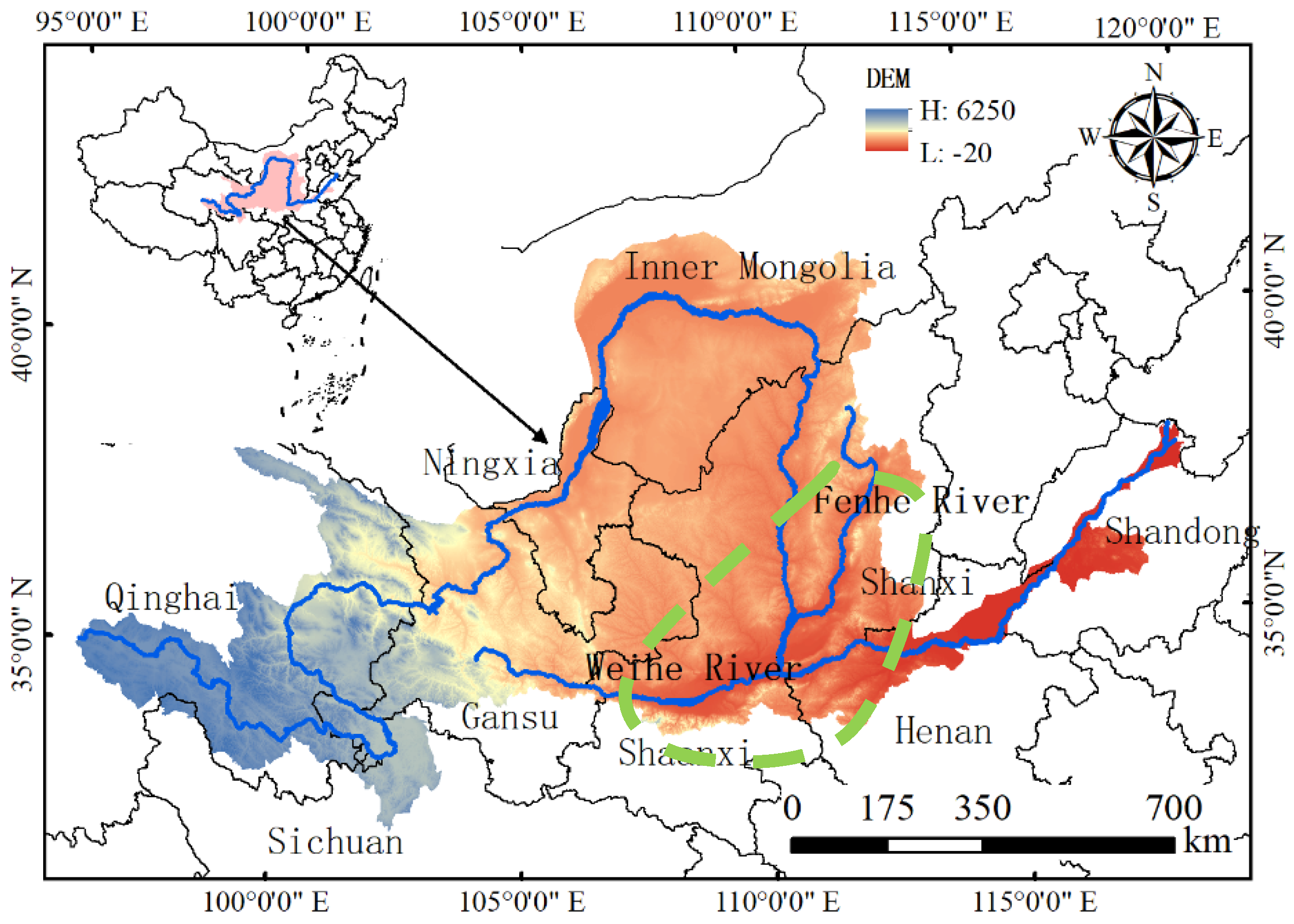
2. Study Area
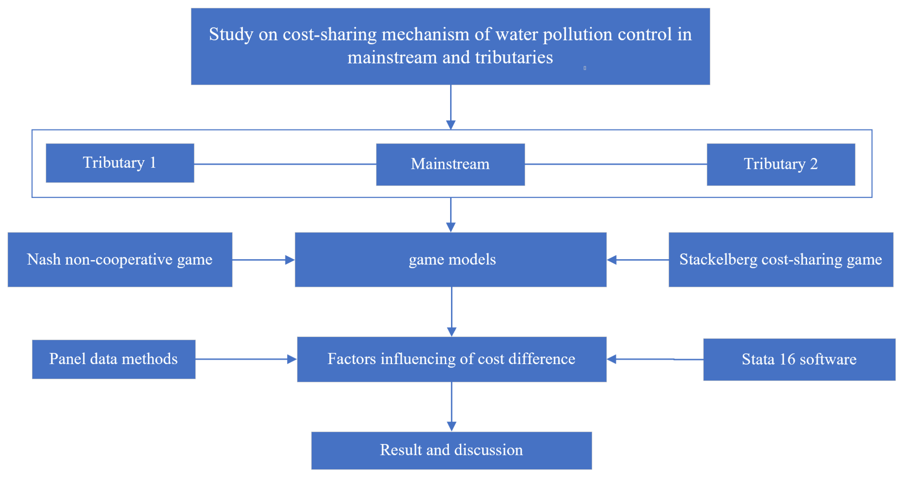
3. Materials and Methods
3.1. Establishment and Solution of Differential Game Models
3.1.1. The Nash Noncooperative Game Scenario
3.1.2. The Stackelberg Cost-Sharing Game Scenario
3.1.3. Numerical Specification
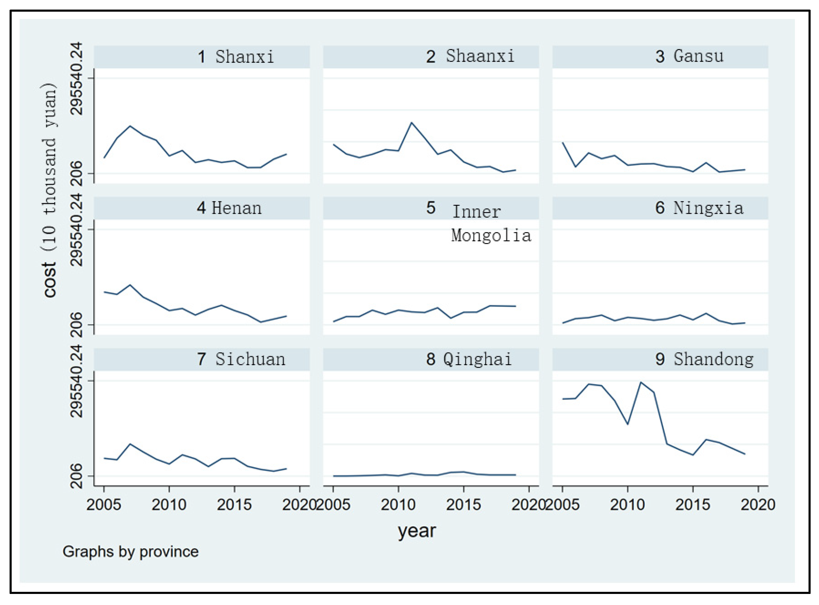
3.2. Factors Influencing Inter-Regional Cost Differences and Coefficient of Cost Difference
3.2.1. Analysis of Factors Influencing Inter-Regional Cost Differences in Pollution Control
3.2.2. The Difference Coefficient for Pollution-Control Costs
4. Results and Discussion
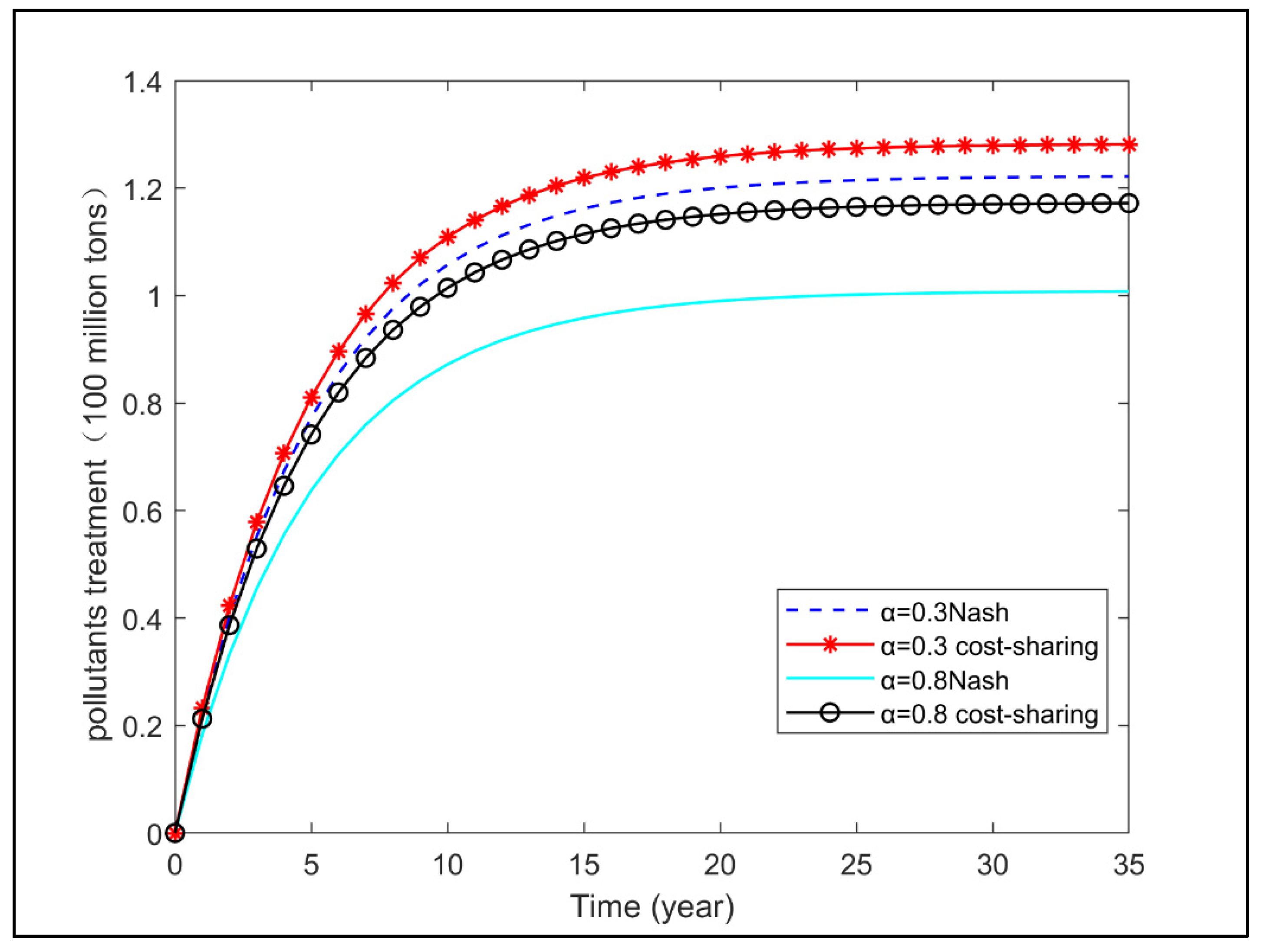
4.1. Comparison of Two Scenarios
4.2. The Influence Law of Competition Coefficient
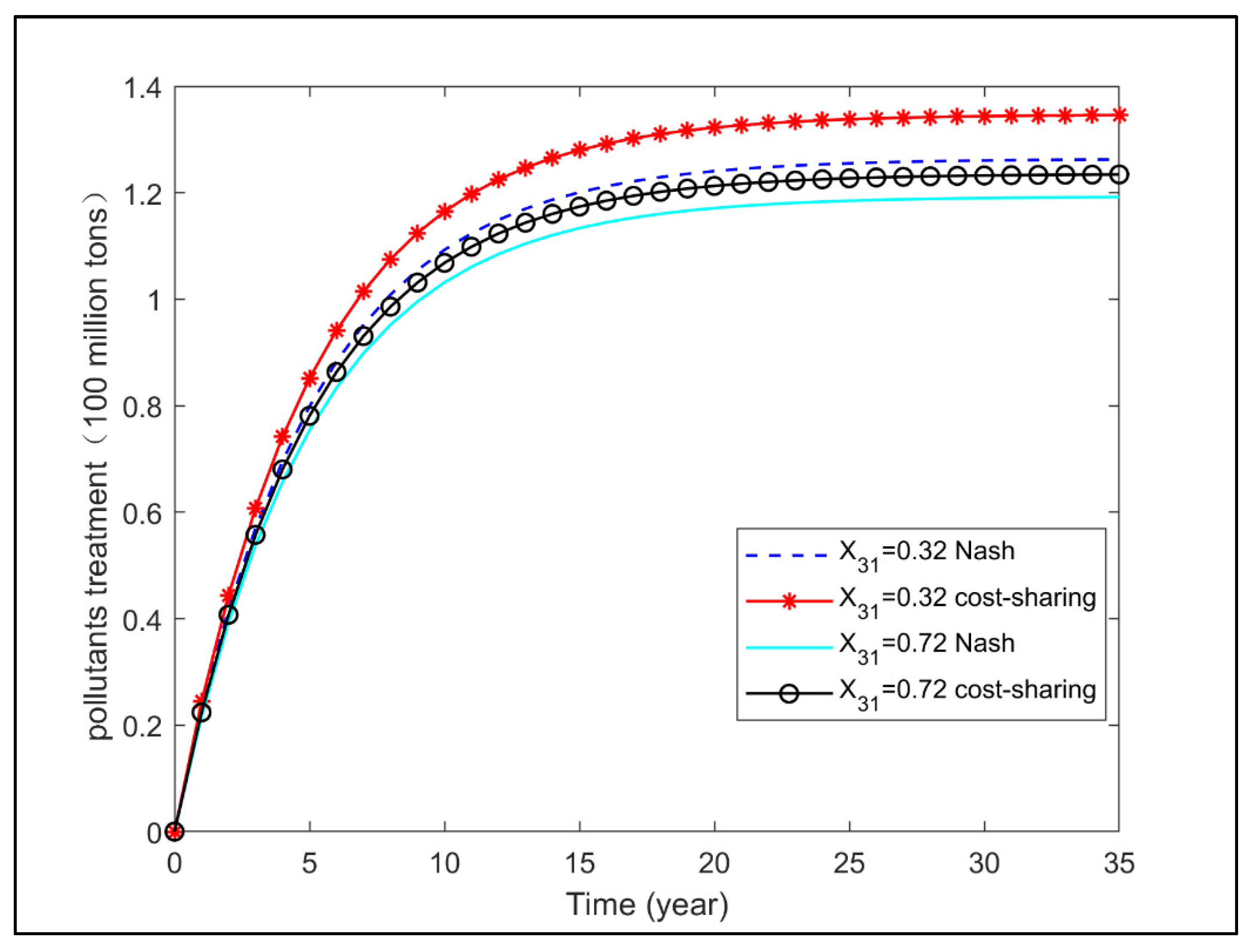
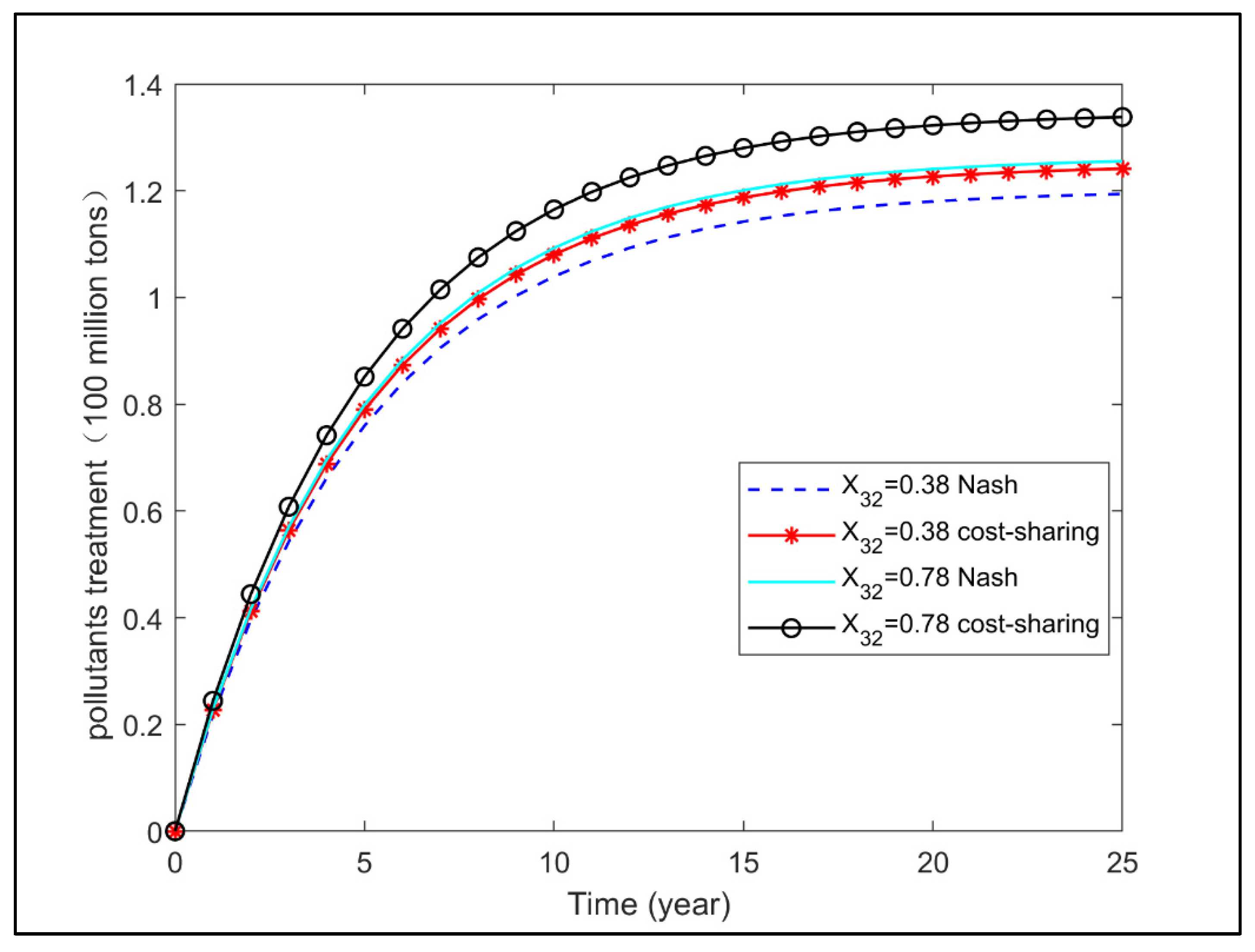
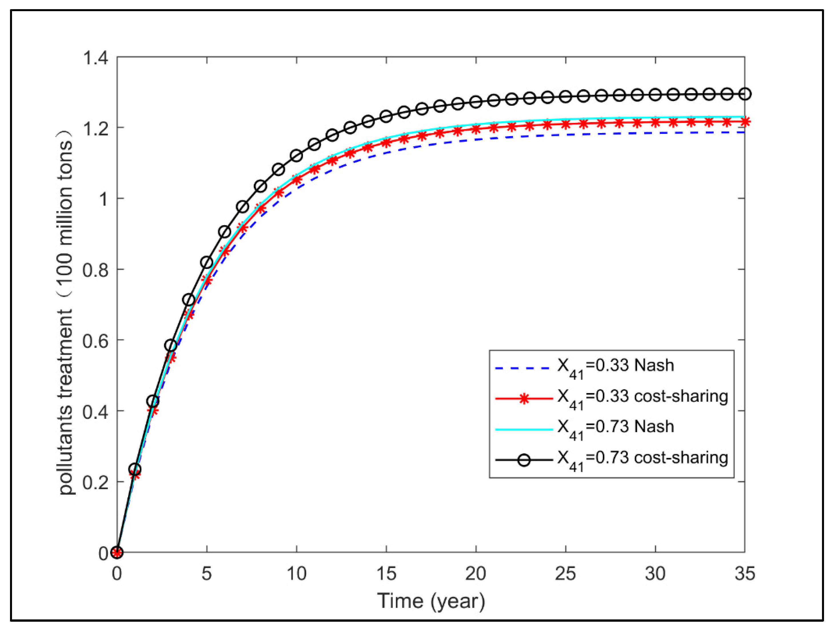
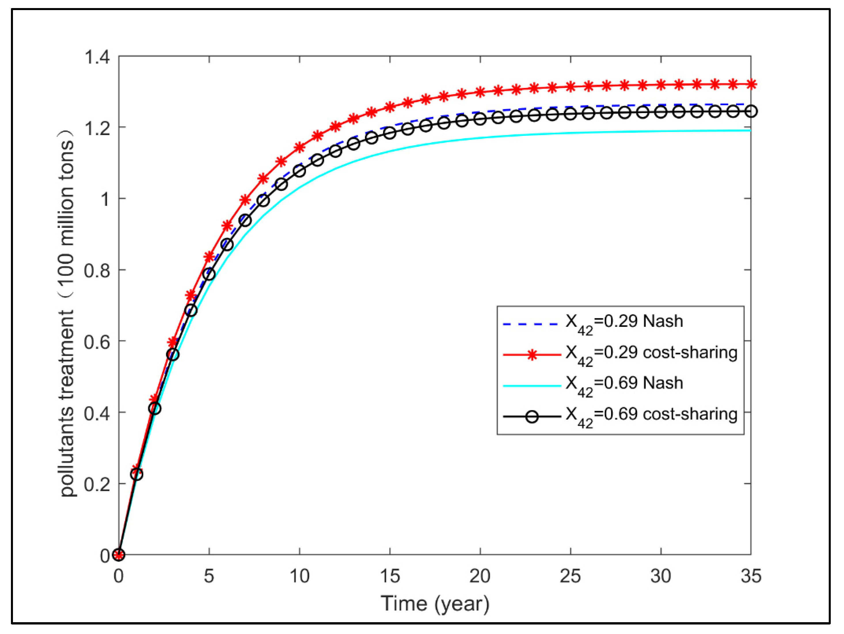
4.2.1. The Effect on Pollutants Treatment
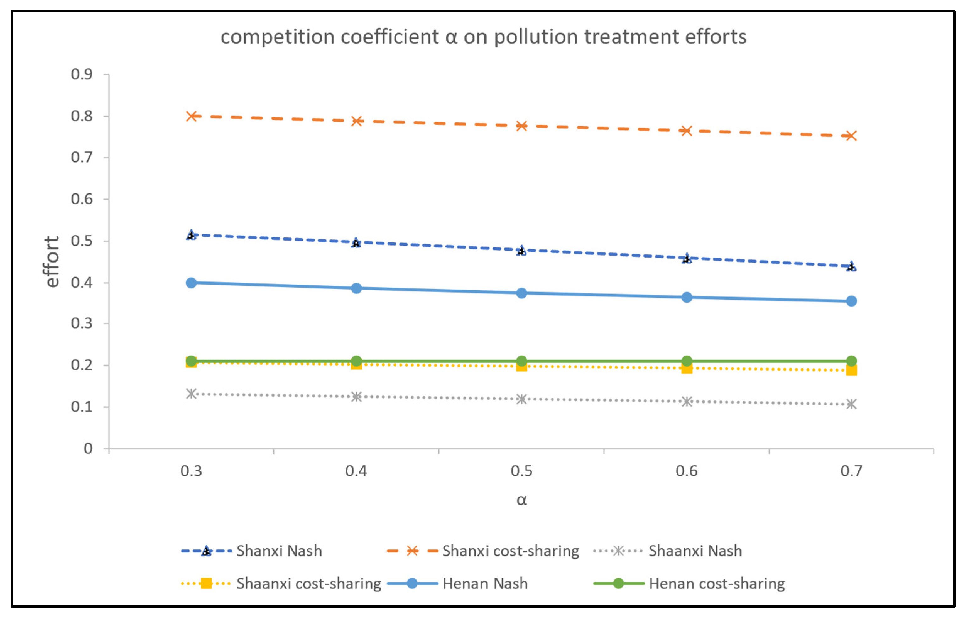
4.2.2. The Effects on the Three Governments’ Pollution-Treatment Efforts
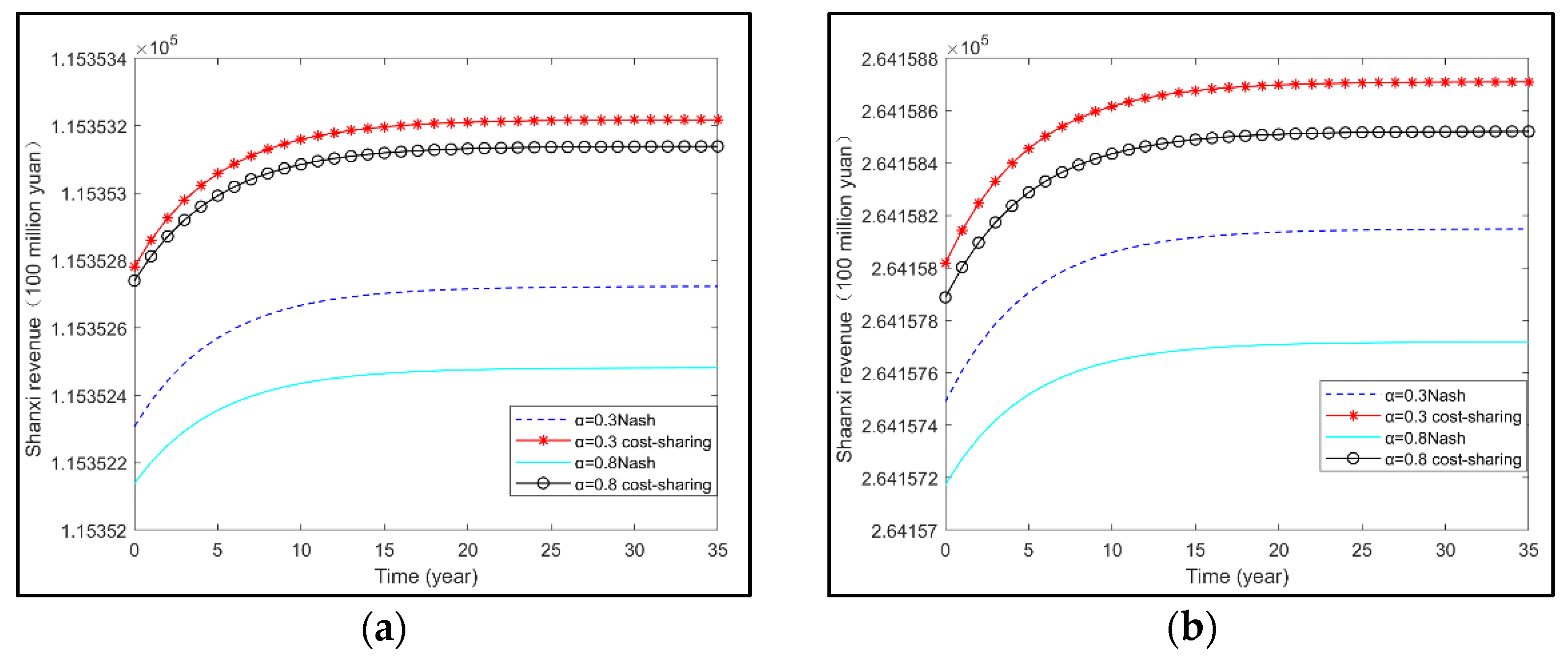
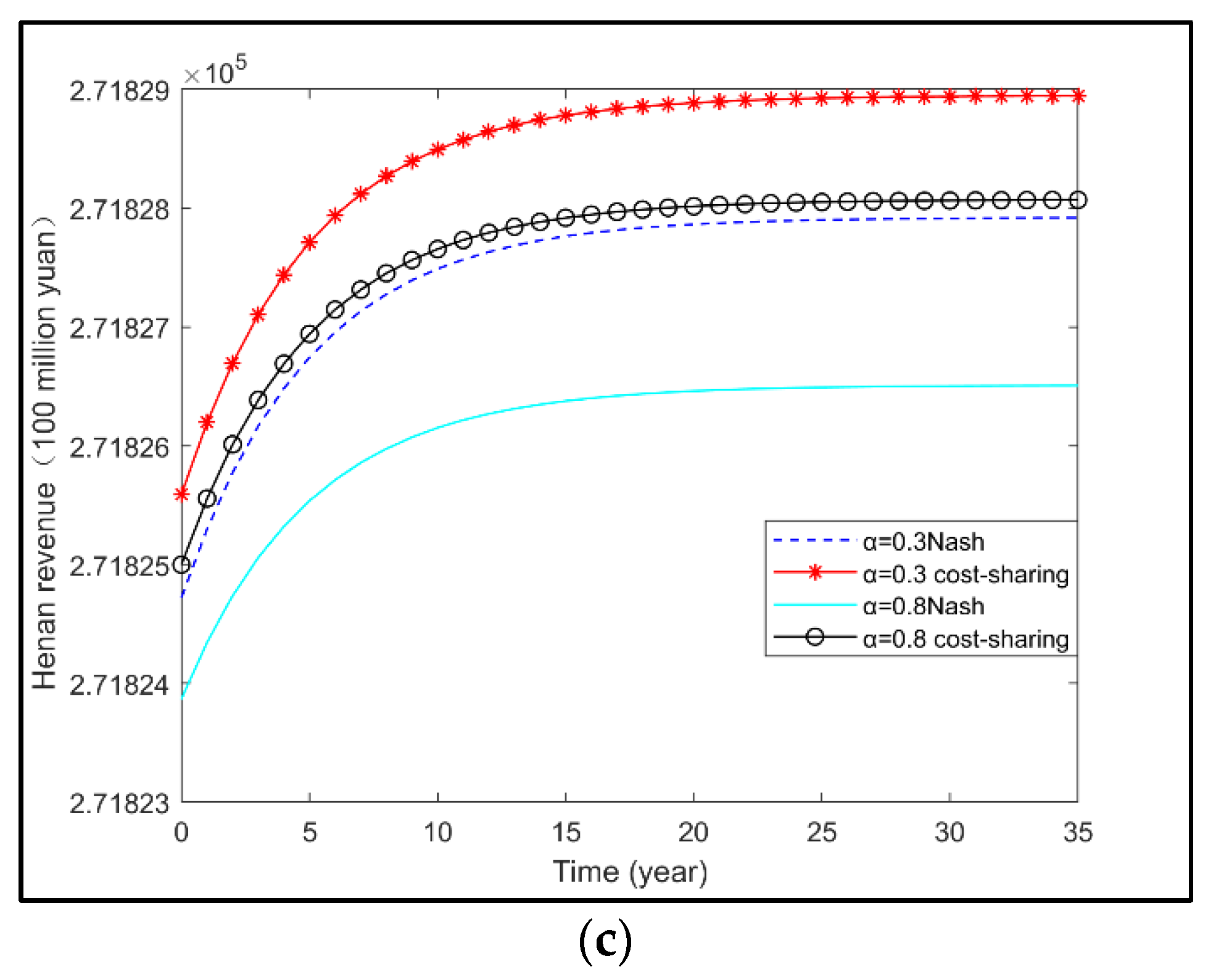
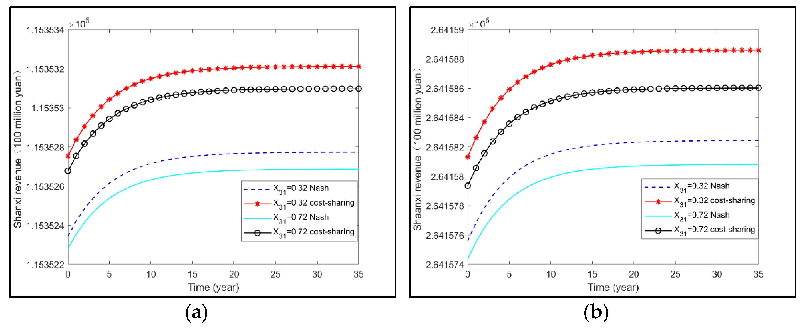
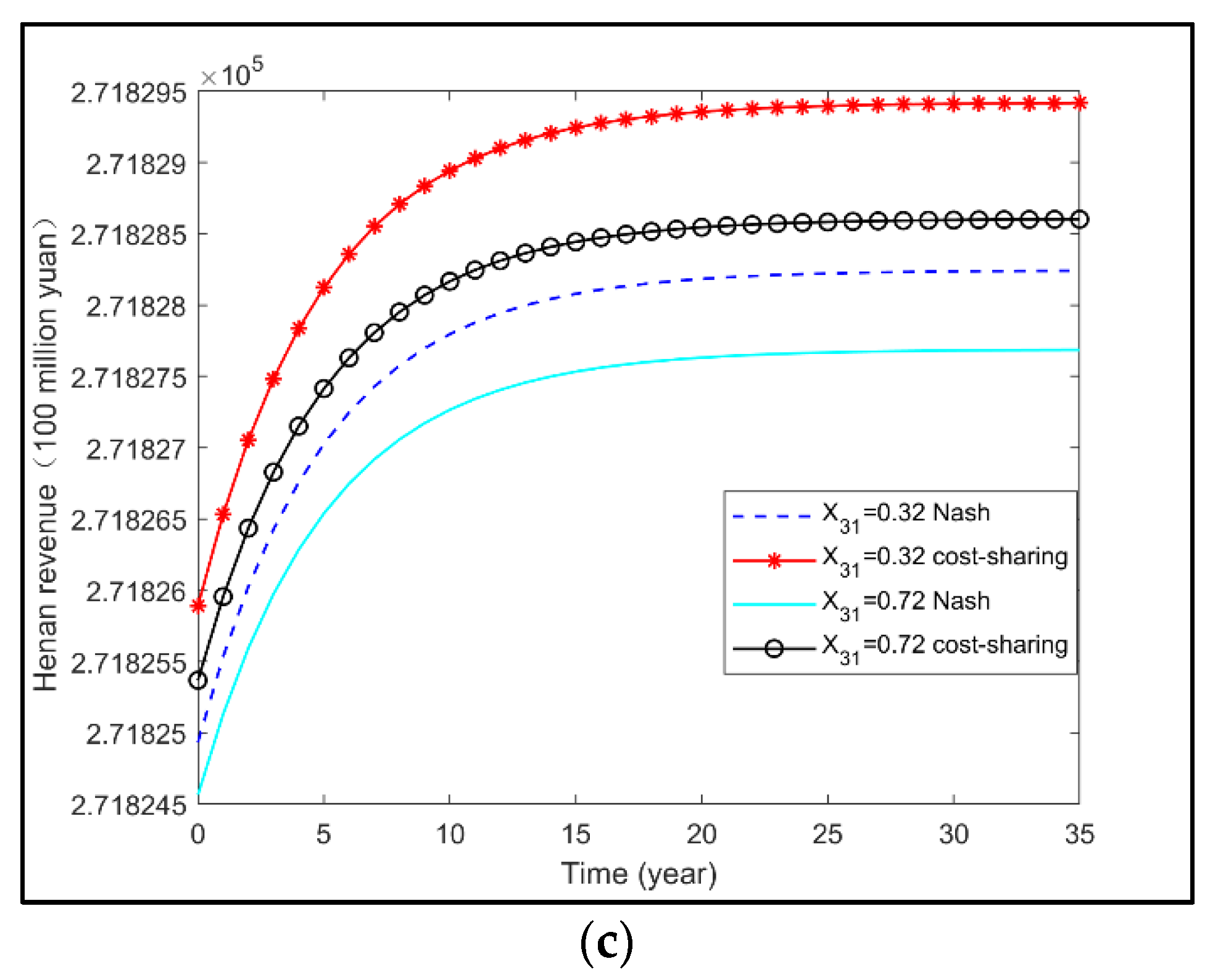
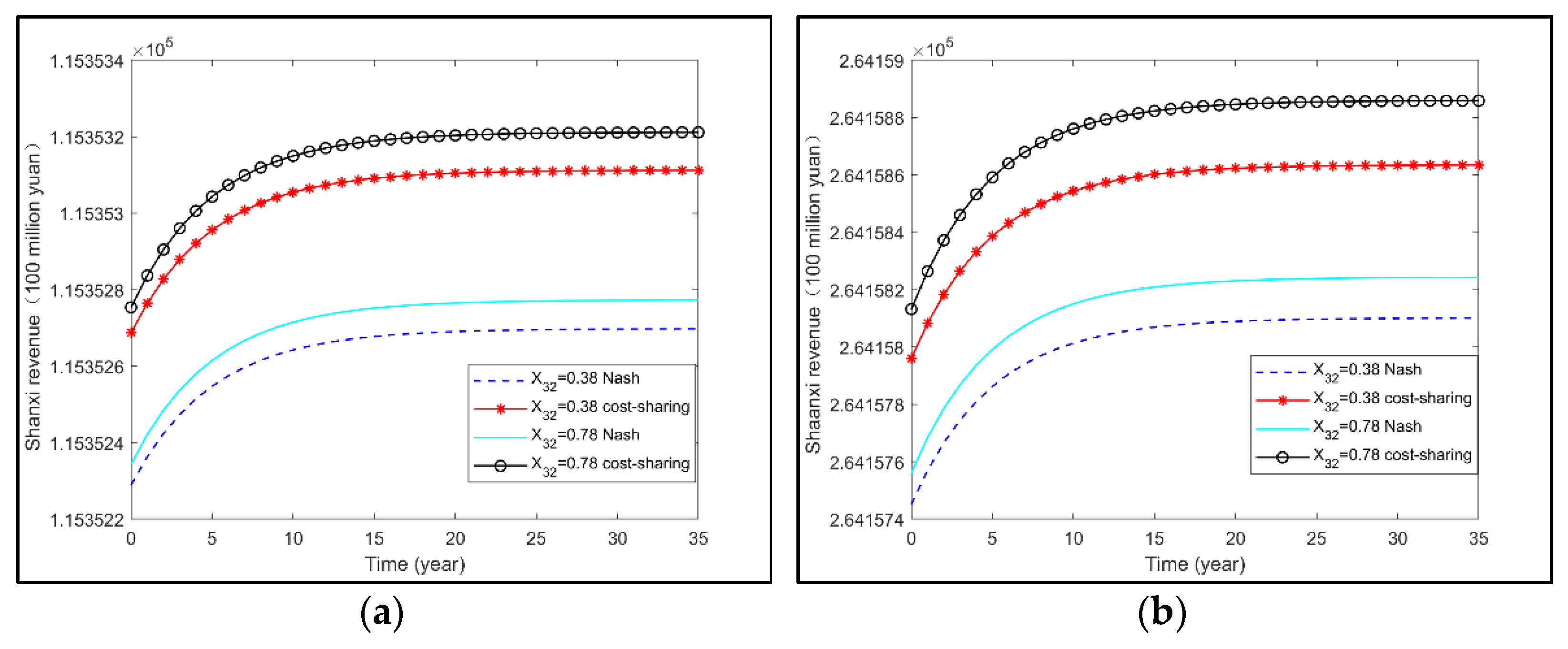
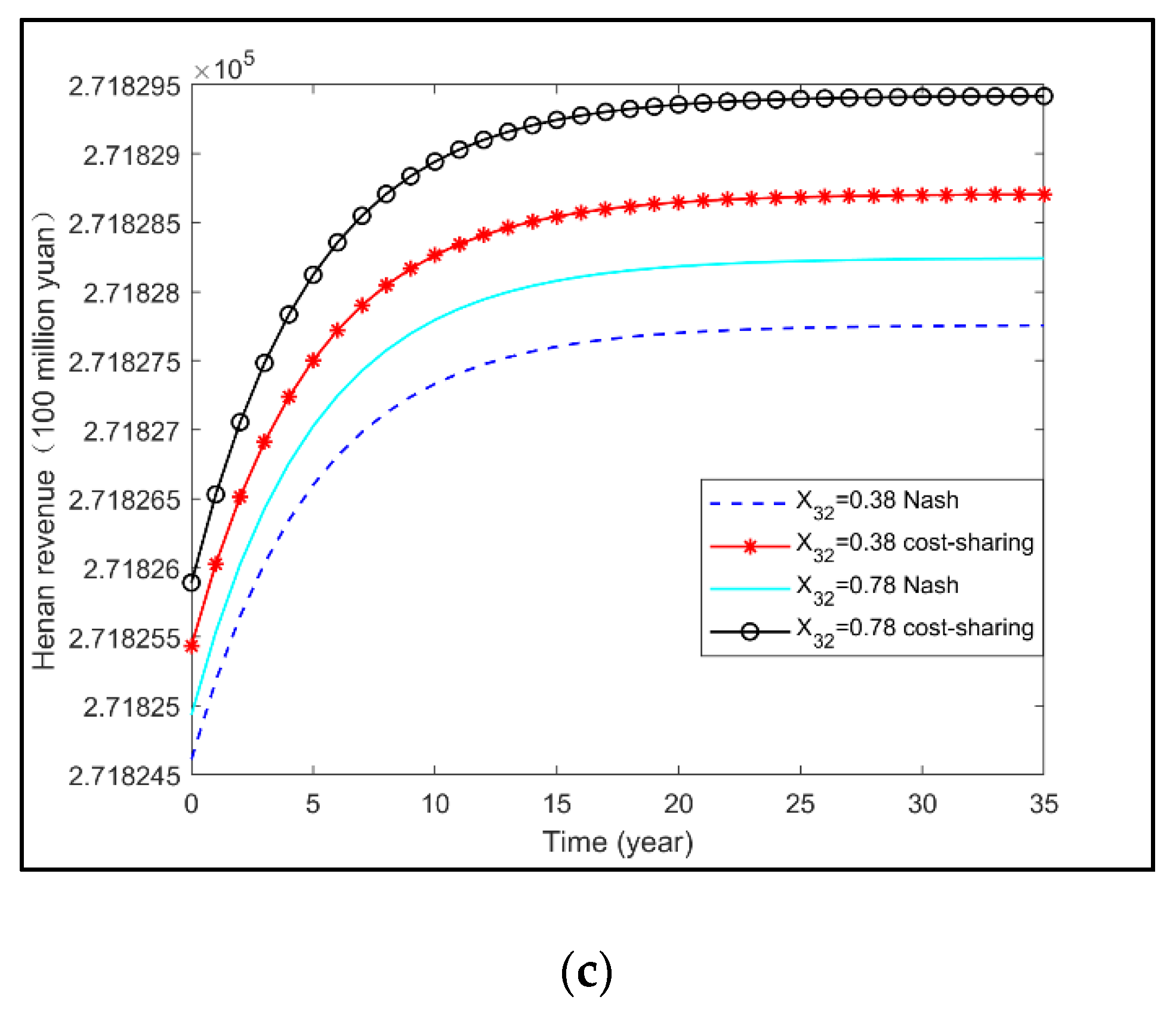
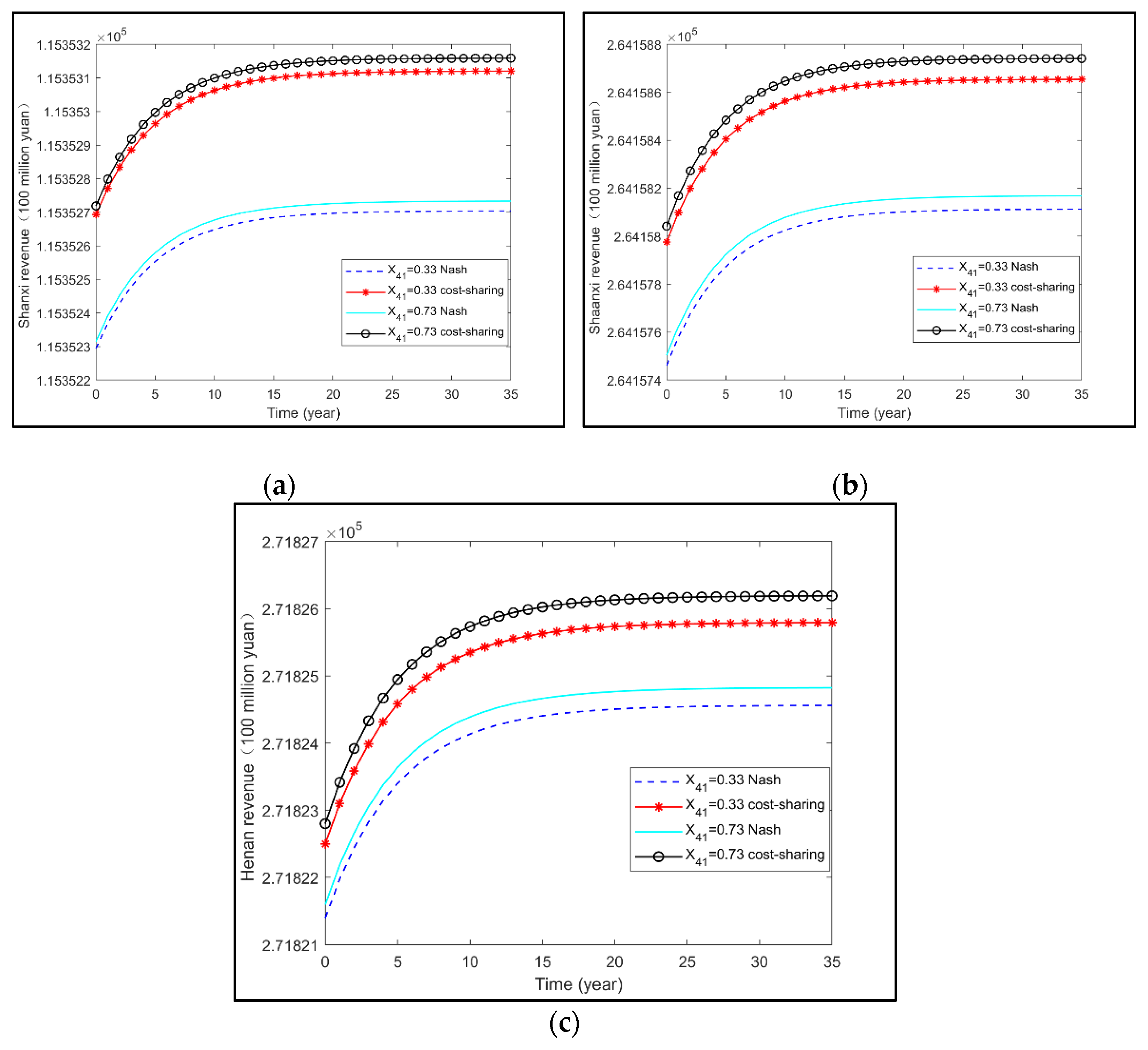
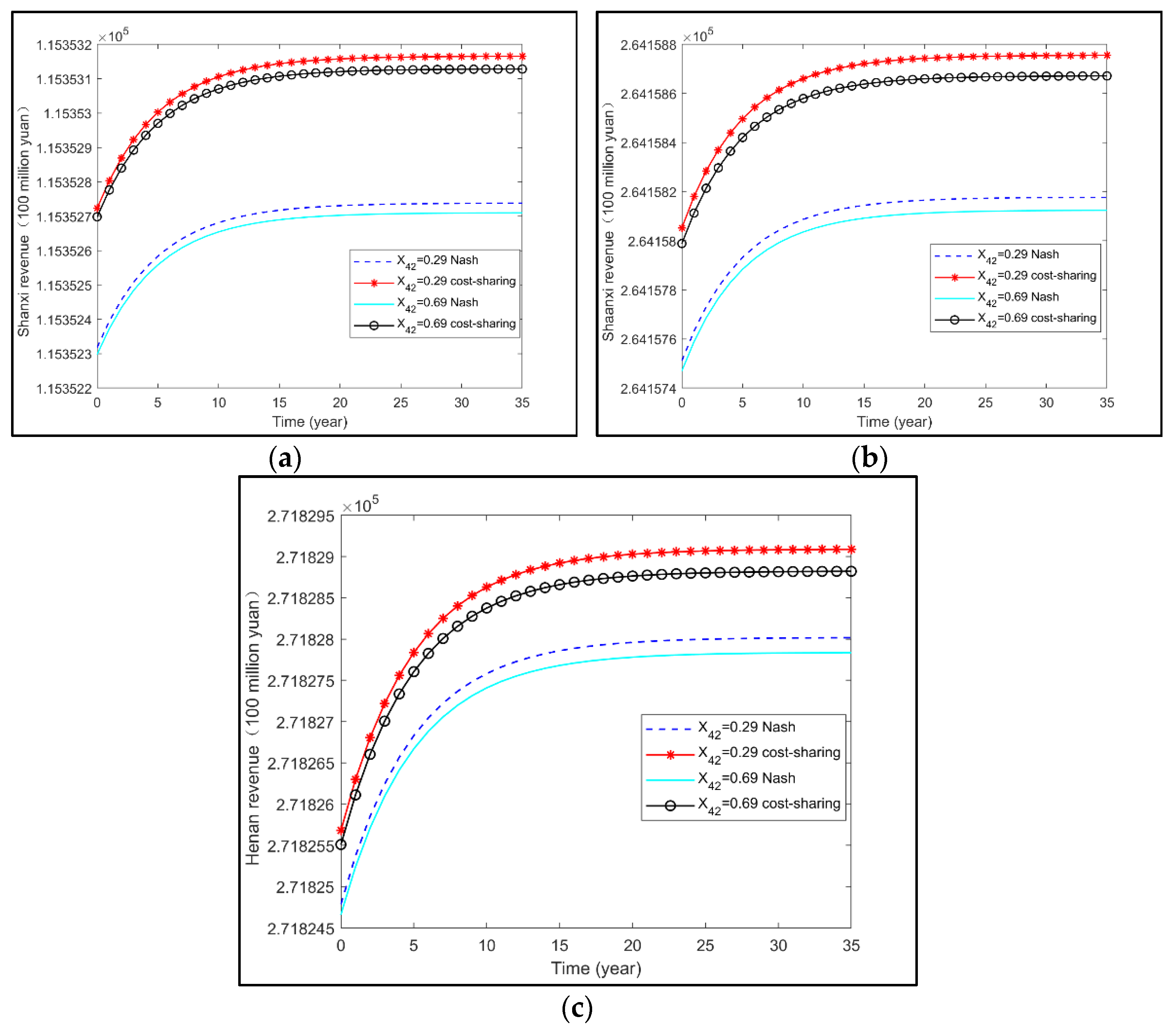
4.2.3. The Effects on the Three Governments’ Revenues
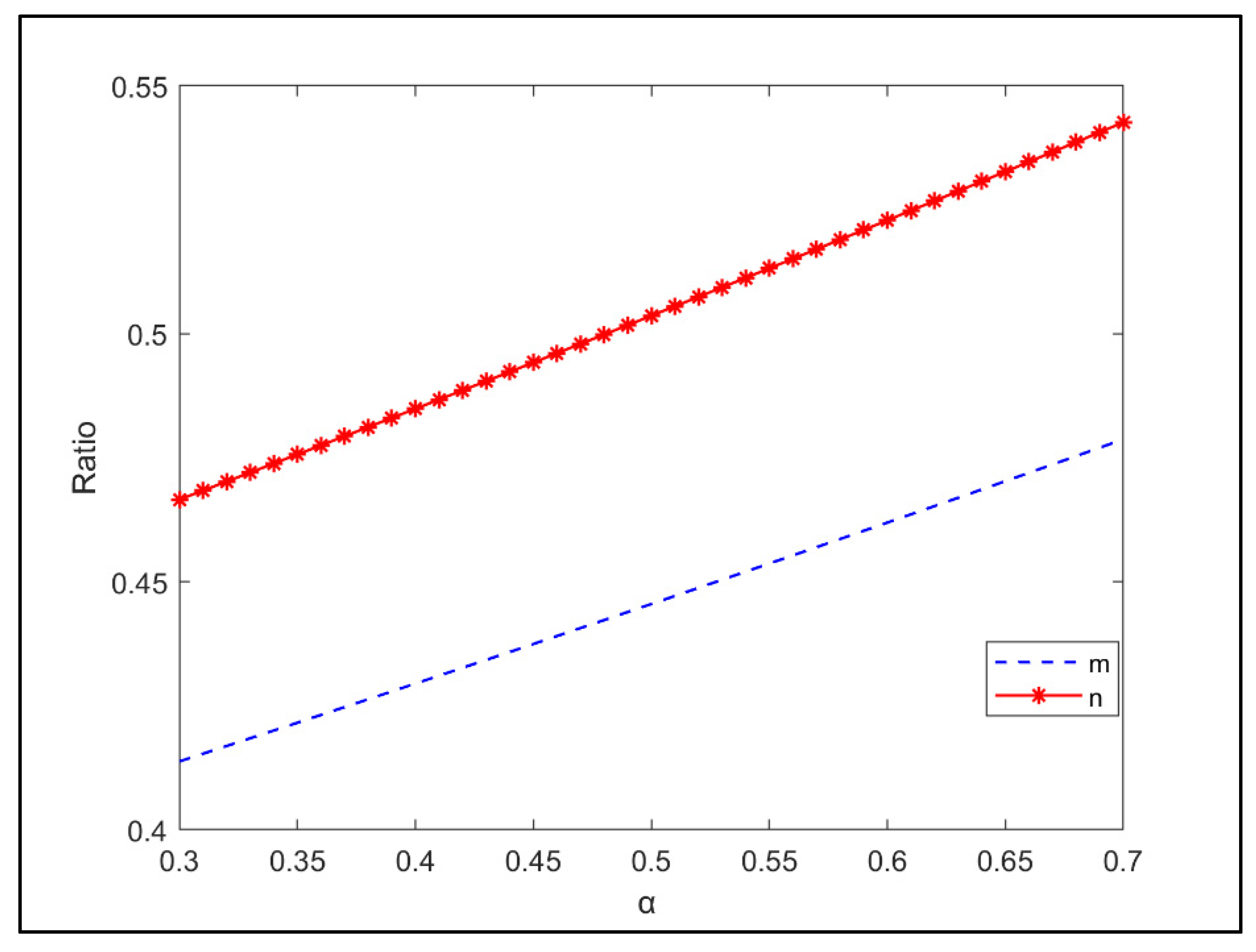
4.2.4. The Effects on Optimal Cost-Sharing Ratio and
4.3. The Influence Law of Urbanization Rate on Pollutants Treated and the Three Governments’ Revenues
4.3.1. The Effects on Pollutants Treated
4.3.2. The Effects on the Three Governments’ Revenues
4.4. The Influence Law of Industrialization on Pollutants Treated and Each Government’s Revenues
4.4.1. The Effects on Pollutants Treated
4.4.2. The Effects on the Three Governments’ Revenues
4.5. Discussion
5. Conclusions
Author Contributions
Funding
Institutional Review Board Statement
Informed Consent Statement
Data Availability Statement
Conflicts of Interest
Appendix A. The Equilibrium Solution under Nash Non-Cooperative Game scenario
Appendix B. The Equilibrium Solution under Stackelberg Cost-Sharing Game Scenario
References
- Sadoff, C.W.; Hall, J.W.; Grey, D.; Aerts, J.C.J.H.; Ait-Kadi, M.; Brown, C.; Cox, A.; Dadson, S.; Garrick, D.; Kelman, J.; et al. Securing Water, Sustaining Growth: Report of the GWP/OECD Task Force on Water Security and Sustainable Growth; University of Oxford: Oxford, UK, 2015. [Google Scholar]
- Valentukeviciene, M.; Bagdziunaite-Litvinaitiene, L.; Chadysas, V.; Litvinaitis, A. Evaluating the impacts of integrated pollution on water quality of the trans-boundary Neris (Viliya) River. Sustainability 2018, 10, 4239. [Google Scholar] [CrossRef] [Green Version]
- Talukder, B.; Hipel, K.W. Diagnosis of sustainability of trans-boundary water governance in the Great Lakes basin. World Dev. 2020, 129, 104855. [Google Scholar] [CrossRef]
- Landrigan, P.J.; Fuller, R.; Acosta, N.J.R. The Lancet Commission on pollution and health. Lancet 2018, 391, 462–512. [Google Scholar] [CrossRef] [Green Version]
- Jiang, D.L.; Cao, G.H. Collusion between government and enterprise in pollution management. J. Syst. Eng. 2015, 30, 584–593. [Google Scholar]
- Hu, Z.Y.; Chen, C.; Wang, H.M.; Zhang, W. Study on differential game and strategy of water pollution control. China Popul. Resour. Environ. 2014, 24, 93–101. [Google Scholar]
- Gao, H.Y. Evolutionary game analysis on water pollution incident based on prospect Theory. Chin. J. Manag. Sci. 2015, 23, 853–859. [Google Scholar]
- Zhu, K.; Zhang, Y.; Wang, M.; Liu, H. The Ecological Compensation Mechanism in a Cross-Regional Water Diversion Project Using Evolutionary Game Theory: The Case of the Hanjiang River Basin, China. Water 2022, 14, 1151. [Google Scholar] [CrossRef]
- Li, G.P.; Wang, Y.Q. ‘Tragedy of the commons’ theory and empirical study in the transboundary water pollution treatment. Soft Sci. 2016, 30, 24–28. [Google Scholar]
- Guan, X.J.; Liu, W.K.; Chen, M.Y. Study on the ecological compensation standard for river basin water environment based on total pollutants control. Ecol. Indic. 2016, 69, 446–452. [Google Scholar] [CrossRef]
- Yu, B.; Xu, L.Y. Review of ecological compensation in hydropower development. Renew. Sustain. Energy Rev. 2016, 55, 729–738. [Google Scholar] [CrossRef]
- Gao, X.; Shen, J.Q.; He, W.J.; Sun, F.H.; Zhang, Z.F.; Guo, W.J.; Zhang, X.; Yang, K. An evolutionary game analysis of governments’ decision-making behaviors and factors influencing watershed ecological compensation in China. J. Environ. Manag. 2019, 251, 109592. [Google Scholar] [CrossRef] [PubMed]
- Gao, X.; Shen, J.Q.; He, W.J.; Sun, F.H.; Zhang, Z.F.; Zhang, X.; Yuan, L.; An, M. Multilevel governments’ decision-making process and its influencing factors in watershed ecological compensation. Sustainability 2019, 11, 1990. [Google Scholar] [CrossRef] [Green Version]
- Sheng, J.C.; Webber, M. Using incentives to coordinate responses to a system of payments for watershed services: The middle route of South–North Water Transfer Project, China. Ecosyst. Serv. 2018, 32, 1–8. [Google Scholar] [CrossRef]
- Yang, Z.; Niu, G.M.; Lan, Z.R. Policy strategy of transboundary water pollution control in boundary rivers based on evolutionary game. China Environ. Sci. 2021, 41, 5446–5456. [Google Scholar]
- Yang, Y.H.; Liu, Y.; Dai, J.; Zeng, Y. Evolutionary Game Analysis of Pollution Emission Reduction in Mainstream and Tributary of Basin under Mechanism of Compensation, Repayment and Reward Integration. Res. Ind. 2022; In press. [Google Scholar]
- Jiang, K.; You, D.M. Study on differential game of transboundary pollution control under regional ecological compensation. China Popul. Resour. Environ. 2019, 29, 135–143. [Google Scholar]
- Jiang, K.; You, D.M.; Li, Z.D.; Shi, S.S. A differential game approach to dynamic optimal control strategies for watershed pollution across regional boundaries under eco-compensation criterion. Ecol. Indic. 2019, 105, 229–241. [Google Scholar] [CrossRef]
- Yi, Y.X.; Wei, Z.J.; Fu, C.Y. A differential game of transboundary pollution control and ecological compensation in a river basin. Complexity 2020, 2020, 6750805. [Google Scholar] [CrossRef]
- Ma, J.; Cheng, C.G.; Tang, Y. Basin eco-compensation strategy considering a cost-Sharing contract. IEEE Access 2021, 9, 91635–91648. [Google Scholar] [CrossRef]
- Li, G.P.; Yan, B.Q.; Wang, Y.Q. Study on environmental regulation strategy evolutionary game for pollution control in the Yellow River basin. J. Beijing Univ. Technol. (Soc. Sci. Ed.) 2022, 22, 74–85. [Google Scholar]
- Han, Y.L.; Lou, G.Y.; Ge, L.; Jin, H.J. Discussion of water-related ecological compensation framework for Yellow River basin. Water Resour. Prot. 2016, 32, 142–150. [Google Scholar]
- Dong, Z.F.; Hao, C.X.; Qu, A.Y.; Liang, Z.M.; Jia, X.R. Orientation and focus on construction of the ecological compensation mechanism in the Yellow River basin. Ecol. Econ. 2020, 36, 196–201. [Google Scholar]
- Yang, Y.X.; Yan, L.; Han, Y.L.; Wang, R.L.; Gao, L.; Zhao, Z.N. Compensation mechanism of the Yellow River water ecology based on watershed scale. Water Resour. Prot. 2020, 36, 18–23. [Google Scholar]
- Zhuang, Y.; Xue, D.Q.; Zhang, R.R. Study on the ecological compensation mechanism of loess plateau in northern shaanxi. Ecol. Econ. 2017, 33, 138–141. [Google Scholar]
- Zhao, Y.Y.; Li, L.Q. An exploration of contents and standard of eco-compensation in the downstream of the Yellow River. Water Resour. Dev. Manag. 2014, 34, 44–46. [Google Scholar]
- Liu, L.Y.; Shi, Z.X.; Ning, L.X. Optimal control model of trans-boundary pollution emissions in two asymmetric countries. Chin. J. Manag. Sci. 2015, 23, 43–49. [Google Scholar]
- Xu, H.; Tan, D.Q. Research on regional cooperative pollution control and dynamic payment distribution strategy. Chin. J. Manag. Sci. 2021, 29, 65–76. [Google Scholar]
- Bai, Z. Econometric Analysis of Panel Data; Nankai University Press: Tianjin, China, 2007. [Google Scholar]
- Guo, S.D.; Tong, M.; Zhang, H. Analysis on the investment efficiency of environmental governance in China and its influencing factors. Stat. Decis. 2018, 34, 113–117. [Google Scholar]
- Li, D.S.; Zhang, Z.Q.; Fu, L.; Guo, S.D. Regional differences in PM2.5 emission reduction efficiency and their influencing mechanism in Chinese cities. China Popul. Resour. Environ. 2021, 31, 74–85. [Google Scholar]
- Gao, J.X.; Wang, Y.C.; Hou, P.; Wan, H.W.; Zhang, W.G. Temporal and spatial variation characteristics of land surface water area in the Yellow River basin in recent 20 years. J. Hydraul. Eng. 2020, 51, 1157–1164. [Google Scholar]
- Zhang, X.Y.; Liu, K.; Wang, S.D.; Wu, T.X.; Li, X.K.; Wang, J.N.; Wang, D.C.; Zhu, H.T.; Tan, C.; Ji, Y.H. Spatiotemporal evolution of ecological vulnerability in the Yellow River Basin under ecological restoration initiatives. Ecol. Indic. 2022, 135, 108586. [Google Scholar] [CrossRef]
- Yang, Y.H.; Fan, J.; Zhu, D.D.; Zhang, Z.N. Study on quality management in three-Level construction supply chain based on differential game. Ind. Eng. Manag. 2021, 26, 96–104. [Google Scholar]
- Li, S. Dynamic optimal control of pollution abatement investment under emission permits. Oper. Res. Lett. 2016, 44, 348–353. [Google Scholar] [CrossRef]
- Li, X.M.; Liu, R.J.; Zhang, Q. Research on cost information sharing and coordination contract of a supply chain with two suppliers and a single retailer. Ind. Eng. Manag. 2021, 26, 1–10. [Google Scholar]
- Yahya, R.; Hadi, S.; Jalal, A.; Ashkan, T. A competitive dual recycling channel in a three-level closed loop supply chain under different power structures: Pricing and collecting decisions. J. Clean. Prod. 2020, 272, 122623. [Google Scholar]
- Dockner Engelbert, J. Van LongNgo. International Pollution Control: Cooperative versus Noncooperative Strategies. J. Environ. Econ. Manag. 1993, 25, 13–29. [Google Scholar] [CrossRef] [Green Version]
- Von Stackelberg, H. Market Structure and Equilibrium (Marktform und Gleichgewicht); Springer: Berlin/Heidelberg, Germany, 1934. [Google Scholar]
- Hu, D.X.; Liu, Z.C.; Liu, T.L.; Liu, Q.P.; Li, Y.J. Analysis on Spatial-Temporal Difference of Water Use Efficiency in Weihe River Basin of Shaanxi Province. Yellow River 2020, 42, 56–61. [Google Scholar]
- Sheng, J.C.; Michael, W. Incentive coordination for transboundary water pollution control: The case of the middle route of China’s South-North water Transfer Project. J. Hydrol. 2020, 598, 125705. [Google Scholar] [CrossRef]
- Liu, H.H.; Wang, N.; Xie, J.C.; Zhu, J.W. Assessment of ecological vulnerability based on fuzzy comprehensive evaluation in weihe river basin. J. Shenyang Agric. Univ. 2014, 45, 73–77. [Google Scholar]
- Zhuang, R.L.; Mi, K.N.; Liang, L.W. China’s industrial wastewater discharge pattern and its driving factors. Resour. Environ. Yangtze Basin 2018, 27, 1765–1775. [Google Scholar]
- Li, Y.X.; Wu, S.; Yan, B.J. Influence mechanism of spatial differentiation of industrial wastewater discharge in China. Environ. Pollut. Control 2021, 43, 1089–1093. [Google Scholar]


| Category | Variables | Description | Measurement | A Priori Sign | |
|---|---|---|---|---|---|
| Explained variable | Investment in industrial sewage treatment | 10,000 yuan | |||
| Explanatory variable | Natural environment | Total amount of water resources | 100 million cu. m | No prediction | |
| Economic development | Per capita GDP (PGDP) | yuan | Negative | ||
| Proportion of urban population to total population at the end of the year | % | Positive | |||
| Value-added of secondary industries as a proportion of regional GDP | % | Positive | |||
| Water consumption of industry | 100 million cu. m | Positive | |||
| Volume of industrial wastewater discharge | 10,000 tons | Positive | |||
| Patent applications granted | piece | Negative | |||
| Variables | Mean | Standard Deviation | Minimum Value | Maximum Value | Observations | |
|---|---|---|---|---|---|---|
| overall | 55,421.39 | 60,419.58 | 206 | 295,540.2 | N = 135 | |
| between | 49,489.11 | 4367.747 | 176,512.6 | n = 9 | ||
| within | 38,173.77 | −54,655.2 | 174,449 | T = 15 | ||
| overall | 568.4675 | 723.2988 | 8.4 | 2953.79 | N = 135 | |
| between | 752.0007 | 10.31033 | 2491.502 | n = 9 | ||
| within | 129.3782 | −57.1945 | 1064.831 | T = 15 | ||
| overall | 32,159.56 | 15,683.06 | 7332 | 70,129 | N = 135 | |
| between | 7283.934 | 19,910.2 | 43,943.6 | n = 9 | ||
| within | 14,087.08 | 5523.956 | 62,375.09 | T = 15 | ||
| overall | 0.4811088 | 0.0830462 | 0.3 | 0.6662526 | N = 135 | |
| between | 0.0578442 | 0.3986667 | 0.5763305 | n = 9 | ||
| within | 0.0624523 | 0.3684421 | 0.5924421 | T = 15 | ||
| overall | 0.4595013 | 0.0618296 | 0.33 | 0.62 | N = 135 | |
| between | 0.0495491 | 0.3909102 | 0.5366667 | n = 9 | ||
| within | 0.0403025 | 0.3528346 | 0.5428346 | T = 15 | ||
| overall | 22.59585 | 18.97095 | 2.4 | 88.56 | N = 135 | |
| between | 19.46974 | 3.946667 | 56.83867 | n = 9 | ||
| within | 4.520003 | 3.697185 | 54.31719 | T = 15 | ||
| overall | 57,135.34 | 54,754.15 | 7098 | 208,257 | N = 135 | |
| between | 55,264.31 | 8163.844 | 172,783.7 | n = 9 | ||
| within | 16,216.13 | −7046 | 100,457.3 | T = 15 | ||
| overall | 20,005.76 | 29,063.94 | 79 | 146,481 | N = 135 | |
| between | 23,018.8 | 887.4667 | 68,127 | n = 9 | ||
| within | 19,240.75 | −37,378.2 | 98,359.76 | T = 15 | ||
| Variables | Statistics | P | |
|---|---|---|---|
| Adjust t * | −5.6423 | 0.0000 | |
| Adjust t * | −3.5988 | 0.0002 | |
| Adjust t * | −2.0491 | 0.0202 | |
| Adjust t * | −4.1176 | 0.0000 | |
| Adjust t * | −2.7843 | 0.0027 | |
| Adjust t * | −1.7622 | 0.0390 | |
| Adjust t * | −3.1458 | 0.0008 | |
| Adjust t * | −6.1683 | 0.0000 |
| Statistical Quantities | Critical Value Corresponding to 5% Significance Level | P | |
|---|---|---|---|
| F(8, 126) | 4.9619833 | 1.6445652 | 0.0000 |
| Variable | Regression Coefficient | T | P |
|---|---|---|---|
| 0.2731058 (0.2778911) | 0.98 | 0.328 | |
| −0.6134181(1.166126) | −0.53 | 0.600 | |
| −1.840621 ** (0.7442428) | −2.52 | 0.018 | |
| 0.6834359 ** (3.165576) | 2.16 | 0.033 | |
| −1.403508 *** (0.3040708) | −4.62 | 0.000 | |
| 0.6229956 * (0.3673876) | 1.74 | 0.085 | |
| −0.4754808 *(0.2891424) | −1.64 | 0.100 |
Publisher’s Note: MDPI stays neutral with regard to jurisdictional claims in published maps and institutional affiliations. |
© 2022 by the authors. Licensee MDPI, Basel, Switzerland. This article is an open access article distributed under the terms and conditions of the Creative Commons Attribution (CC BY) license (https://creativecommons.org/licenses/by/4.0/).
Share and Cite
Yang, Y.; Liu, Y.; Yuan, Z.; Dai, J.; Zeng, Y.; Khan, M.Y.A. Analyzing the Water Pollution Control Cost-Sharing Mechanism in the Yellow River and Its Two Tributaries in the Context of Regional Differences. Water 2022, 14, 1678. https://doi.org/10.3390/w14111678
Yang Y, Liu Y, Yuan Z, Dai J, Zeng Y, Khan MYA. Analyzing the Water Pollution Control Cost-Sharing Mechanism in the Yellow River and Its Two Tributaries in the Context of Regional Differences. Water. 2022; 14(11):1678. https://doi.org/10.3390/w14111678
Chicago/Turabian StyleYang, Yaohong, Ying Liu, Zhen Yuan, Jing Dai, Yi Zeng, and Mohd Yawar Ali Khan. 2022. "Analyzing the Water Pollution Control Cost-Sharing Mechanism in the Yellow River and Its Two Tributaries in the Context of Regional Differences" Water 14, no. 11: 1678. https://doi.org/10.3390/w14111678