Innovative Trend Analysis of Air Temperature and Precipitation in the Jinsha River Basin, China


1
College of Hydrology and Water Resources, Hohai University, Nanjing 210098, China
2
Department of Civil Engineering, Curtin University, Perth 6102, Australia
3
CSIRO Land and Water, Private Bag 5, Wembley 6913, Australia
4
College of Urban and Environmental Science, Northwest University, Xi’an 710127, China
*
Author to whom correspondence should be addressed.
Water 2020, 12(11), 3293; https://doi.org/10.3390/w12113293
Submission received: 21 September 2020
/
Revised: 6 November 2020
/
Accepted: 20 November 2020
/
Published: 23 November 2020
(This article belongs to the Section Hydrology)
Abstract
:Trend detection based on hydroclimatological time series is crucial for understanding climate change. In this study, the innovative trend analysis (ITA) method was applied to investigate trends in air temperature and precipitation over the Jinsha River Basin (JRB), China, from 1961 to 2016 based on 40 meteorological stations. Climatic factors series were divided into three categories according to percentile, and the hidden trends were evaluated separately. The ITA results show that annual and seasonal temperatures have significantly increased whereas the variation range of annual temperature tended to narrow. Spatial pattern analysis of the temperature indicates that high elevation areas show more increasing trends than flat areas. Furthermore, according to ITA, significant increase trends are observed in annual precipitation and “high” category of spring precipitation. The sub-basins results show a significant decreasing trend in elevation zones of ≤2000 m and an increasing trend where elevation is >2000 m. Moreover, linkage between temperature and precipitation was analyzed and the potential impact of the combined changes was demonstrated. The results of this study provide a reference for future water resources planning in the JRB and will help advance the understanding of climate change in similar areas.
1. Introduction
Climate change is a global issue [1]. Air temperature and precipitation are the most important variables to hydrometeorology, which can be used to understand the climate of a region and assess the effects of climate change [2]. Climate change, together with anthropogenic activities, serves as one of the main driving forces of the hydrological cycle [3,4,5]. For instance, warming temperatures could result in changes to glacial melting [4,6] and evapotranspiration [4,7]. Furthermore, the amount and frequency of precipitation directly controls river discharge [8]. Trend identification methodologies enable the identification and interpretation of climate change effects [9], and there is a growing need to identify trends in air temperature and precipitation at different spatial and temporal scales to manage regional water resources and related hazards more effectively.
Trends within climatic variable time series have received considerable attention in recent decades [10] and have been investigated using different methodologies, including parametric and/or nonparametric procedures, such as the Mann–Kendall (MK) test [11,12,13], linear regression method [6,14], and the Theil–Sen approach (TSA) [15,16]. Su et al. [17] employed linear regression and the MK approach to detect trends in annual and seasonal temperature and precipitation extremes over the Yangtze River Basin (YRB). The MK along with the TSA method were applied by Gocic and Trajkovic [16] to study seven annual and seasonal meteorological variable trends in Serbia. Also based on the MK method, Chowdhury et al. [18] and Jones et al. [19] analyzed annual and seasonal precipitation trends in the South Australian and Upper Tennessee River basins, respectively. However, traditional methods are limited by their use of time series data, which have serial correlations [20]. Besides, these methods can only show monotonical trends through pure statistical calculations; they are unable to identify trends in different categories of value within one calculation process [21]. Therefore, it is necessary to verify the trends calculated by traditional methods and to reveal hidden trends in low, medium, and high value categories by using flexible graphical techniques.
Recently, the innovative trend analysis (ITA) method introduced by Sen [22,23,24] has been widely used for studying trends of hydrological and meteorological variables in many regions [25,26,27,28,29]. The method is simple, intuitive, can be employed irrespective of distribution assumptions, and has the ability to identify trends of different subcategories. Sonali and Nagesh Kumar [25] found that significant hidden subtrends of the annual and monthly temperature in India could be obtained by the graphical ITA method. The ITA method was used to investigate trends in pan evaporation in Turkey [26], and the advantages of ITA in examining trends in low, medium, and high categories was emphasized. Caloiero et al. [29] applied the ITA method to investigate trends in low, medium, and high rainfall values in southern Italy; they confirmed that ITA has advantages in identifying the trends of different categories compared with the MK test. Sen [24] further proposed a formulation to calculate monotonic trends and developed a significance test for ITA; based on this work, it is now easier to analyze trends in low, medium, and high categories.
Data series need to be divided into subcategories to analyze hidden trends. There are three approaches for this division. (1) Elouissi et al. [30] defined subcategories according to the absolute value of the data, and divided the maximum value of the horizontal axis into three equal parts (low, medium, and high). (2) Güçlü [31] classified subcategories according to differences in the trends, and introduced the Pettitt test to divide low and high categories objectively. (3) Wu and Qian [28] divided rainfall intensities into five categories and Wang et al. [10] divided rainfall into three categories based on percentiles. Division based on percentiles not only avoids subcategories with no data, but also specifies the number of data in each subcategory, which facilitates the comparison of data series [10].
Many studies have investigated trends in global temperatures and global warming, and the impact of this phenomenon has been widely discussed [1,32]. The trends in global precipitation are more complex, and different conclusions have been drawn in previous studies [33,34]. For instance, Phu et al. [33], based on satellite observations from 1983 to 2015 and MK methods, pointed out that while there were regional trends, there was no evidence for an increase in precipitation at the global scale in response to the observed global warming. However, based on historical reconstructed precipitation data from 1900 to 2008, Ren et al. [34] found significant increasing trends in global annual mean precipitation in both the reconstruction and model simulations, including CMIP3 and CMIP5. The temperature and precipitation changes in China have also been a continuous research concern [6]. Additionally, the trends in temperature and precipitation in the Yangtze River, which is the largest river in China and the third largest river in the world, have been widely studied [8,35].
The Jinsha River is the “water tower” of the Yangtze River, and climate change in the Jinsha River Basin (JRB) has been investigated by various studies. Wang and Zhang [36] applied a linear trend analysis and the MK method to analyze the annual and seasonal temperature trends in the JRB from 1961 to 2008 based on aggregated mean temperatures of 30 meteorological stations. Their results showed that there was an increasing trend in the annual and seasonal temperatures, with the increase in winter temperatures being more significant than that during the other seasons. Wang et al. [37] applied the MK method to study for the first time the precipitation trend in the JRB at different temporal and spatial scales. They concluded that there was a nonsignificant increasing trend in annual precipitation, while the increasing trend during spring was more significant than those during the other seasons. Various other studies [38,39,40] have also applied the MK approach to investigate trends in climatic variables such as temperature and precipitation in the JRB. However, a limited number of studies have focused on spatial and temporal variations in different categories of temperature and precipitation, especially for the low and high categories. The trends of the low and high categories of temperature are important signals for the occurrence of heat waves and cold snaps, which presents a challenge for agricultural management. Moreover, the occurrence of floods and droughts is highly related to the low and high categories of precipitation [10], which represents a challenge for water resources management.
The JRB has a large elevation range (up to 5142 m) and contains more than 40 meteorological stations, all of which have long term (>50 years) observation data. Thus, the JRB is an ideal place to identify the impact of elevation on trends in climatic factors. Some researchers have reported that high altitude areas show greater increases in air temperature than do plain areas [41,42], whereas some researchers reported opposite patterns [43]; however, other studies have suggested that there is no clear relationship between trend magnitudes and elevation [44,45]. As such, the impact of elevation on precipitation in the JRB requires further study. Moreover, the relationship between subcategory trends and elevation has not been studied previously. The relationship between elevation and trends in climatic factors can not only provide information about climate change in the JRB, but can also help to understand climate change in other similar mountain areas, which often lack data owing to observation difficulties.
The long-term tendencies of the annual and seasonal minimum temperature (Tmin) and maximum temperature (Tmax) are critical for detecting and quantifying the potential impacts of climate change and for long-term planning of climate change adaption on a regional scale [46]. Thus, in this study, Tmin and Tmax were analyzed separately rather than considering the mean temperature alone, as done by the majority of previous studies [38]. Most past studies analyzed either precipitation or temperature; those considering a combination of precipitation and temperature, including their covariability, are limited [2]. Thus, the possible spatiotemporal relationship between precipitation and temperature regimes was also evaluated in this study.
This study aimed to: (1) investigate climate change in the JRB using a trend analysis of annual and seasonal air temperature (minimum and maximum) and precipitation based on observational data from 1961 to 2016; (2) quantitatively evaluate trends in low, medium, and high categories of annual and seasonal air temperature and precipitation; (3) analyze spatial patterns of annual climatic factor trends and identify the impact of elevation; and (4) evaluate possible spatiotemporal relationships between temperature and precipitation. The null hypothesis H0 in this study was that no significant trend at a 95% confidence level would occur for an independent and identically distributed time series [34]. The results of this study are expected to enhance the understanding of climate change within the JRB and the linkage between climate change and the hydrological cycle. Moreover, these results provide an important resource for water resource management, climate change adaptation strategy formulation, and socioeconomic development in similar regions.
2. Materials and Methods
2.1. Study Area and Observation Data
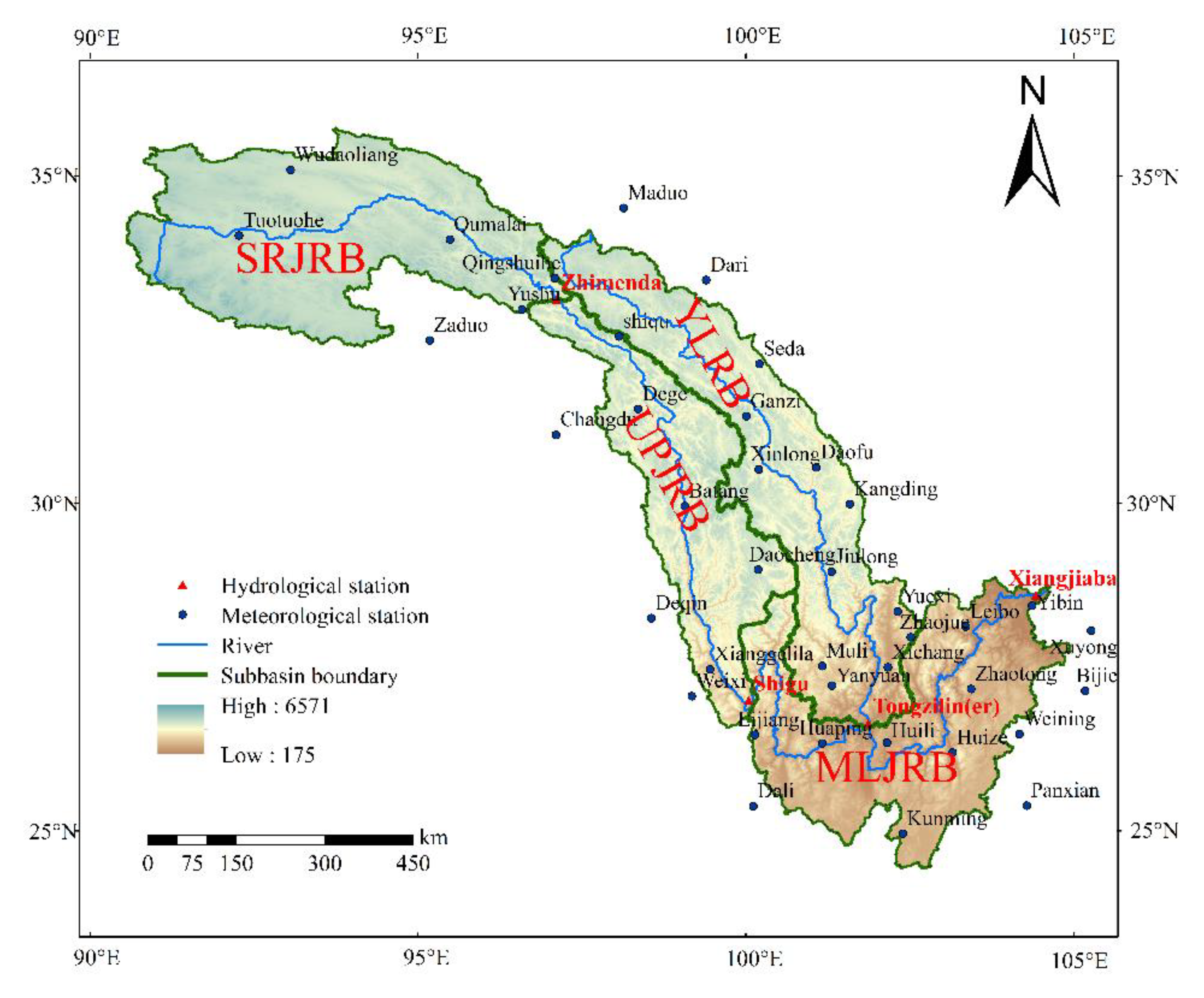
The JRB, covering an area of 473,200 km2, is the uppermost part of the YRB and accounts for 26% of the latter’s total drainage area [35]. The JRB is located in southwestern China and extends between 24°36′–35°44′ N and 90°30′–105°15′ E, with an elevation difference of up to 5142 m (Figure 1). The northwestern part of the JRB belongs to the Qinghai–Tibet Plateau, which is an active area for studying the impact of global warming. Furthermore, increases in the amount of glacier melt runoff have been reported in the northwestern part of the JRB [47]. The southeastern part of the JRB covers the provinces of Yunnan and Sichuan [38]. The Jinsha River has a length of 3464 km; the mainstream of the JRB accounts for 77% of the length of the upper Yangtze River [37]. The Yalong River is the largest tributary of the Jinsha River, with both rivers merging at Panzhihua City, Sichuan Province. Human-induced land cover change is reported to have an impact on the regional climate [48]; however, Yin et al. [49] pointed out that for the whole JRB, the share of each primary land use category did not vary notably from 1975 to 2000. Additionally, from 1970 to 2017, land use change exerted little impact on runoff extremes, while climate change was one of the main factors that led to changes in extreme hydrological situations [50].
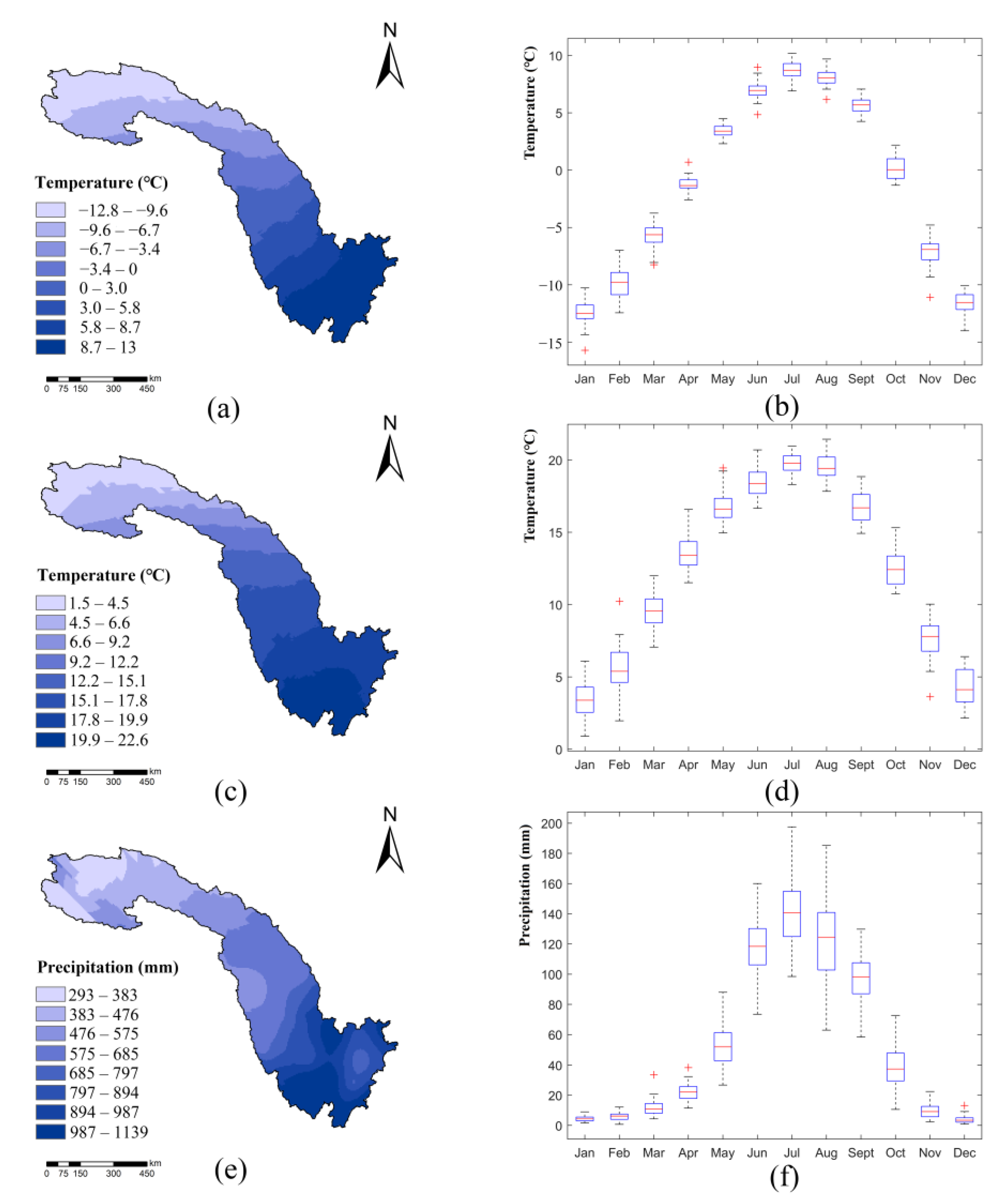
Annual air temperature and precipitation in the JRB have a high spatial variability, where the southeastern JRB is warmer and wetter than the northwestern area (Figure 2a,c,e). The mean annual Tmin is −12.8–1.3 °C, and the mean annual Tmax is 1.5–22.6 °C. The average annual rainfall ranges from 293 mm in the northwest to 1139 mm in the southeast. The northwestern part of the JRB lies in an arid zone, while the middle and lower part of the JRB lie in an Indian monsoon dominated zone [38]. The temporal variations in Tmin, Tmax, and precipitation show that the summer is hot and wet, whereas the winter is cold and dry (Figure 2b,d,f). Precipitation is concentrated in the wet season (June to September), during which 75.7% of the annual total precipitation occurs.
The data used in this study were obtained from the China Meteorological Administration (Appendix A), which applies data quality control before releasing these data [51]. Without adequate quality control, the identified climatic trends have in fact been spurious or unverified [52]. Thus, in this study, data quality control checks were performed using RClimDex (http://etccdi.pacificclimate.org/software.shtml (accessed on 15 September 2020) and any potential outliers identified (such as typing errors, missing data, rejected values, and minimum values greater than maximum values) were manually checked and corrected. In addition, the total number of missing monthly data was 28 among the 40 stations and 56 year study period, which was about 0.10% of data used. (http://data.cma.cn/article/showPDFFile.html?file=/pic/static/doc/A/SURF_CLI_CHN_MUL_MON/SURF_CLI_CHN_MUL_MON_STATION.pdf, in Chinese, (accessed on 15 September 2020)).
In this study, the run homogeneity test proposed by Swed and Wisenhart [53] was applied to determine the homogeneity of the data at a 5% significance level [31]. When the variations in climatic factor series only result from the changes in climate and air, the climate record is considered homogeneous [54]. However, nonclimatic factors such as station relocations, changes in site conditions (land use/forest growth), modifications in the instrumentation and recalibrations, or variations in observation procedures, often affect the observed time series [55]. Without a homogeneity test, the impact of nonclimatic factors can mask or even mismatch the real climate change in the time series. Thus, a homogeneity test is important and essential for trend analysis studies of hydrometeorological variables [54]. The run homogeneity test is expressed as follows [31]:
where ZR is the run homogeneity test result, R is the run number, N1(N2) is the number of values below (above) the median, and N is the number of datapoints. When the calculated ZR value is within 5% significance level, the data are nonhomogeneous. Herein, only homogeneous data were used to identify trend conditions [31].
Among the 60 National Meteorological Observatory stations in or around the JRB, 40 stations were found to be homogeneous by the run homogeneity test on monthly air temperature and precipitation series at the 95% confidence level and had a continuous data series from 1961 to 2016. Thus, these 40 stations were selected to analyze the trends in air temperature and precipitation in the JRB. The geographical information of the meteorological stations is listed in Table 1 and the locations of the meteorological stations are shown in Figure 1.
In this study, the meteorological factors included the monthly average minimum temperature (Tmin), the monthly average maximum temperature (Tmax), and the monthly precipitation. Spring was defined as March to May, summer from June to August, autumn from September to November, and winter from December to February of the following year. Based on a digital elevation model and the distribution of hydrological stations, the JRB was divided into four sub-basins (Figure 1): the source region of the JRB (SRJRB), the upper part of the JRB (UPJRB), the Yalong sub-basin (YLRB), and the middle and lower parts of the JRB (MLJRB). The regional mean air temperature and precipitation were calculated using the Thiessen polygon method based on observations from 40 meteorological stations [38,50].
2.2. Trend Analysis Methods
2.2.1. Innovative Trend Analysis (ITA)
Using ITA, a time series can be divided into two equal halves, with both subseries sorted separately and in ascending order. Based on the Cartesian coordinate system, the first subseries (x) is placed on the X axis, and the second subseries (y) is placed on the Y axis (Figure 3). If the data points are located on a 1:1 straight line (i.e., the two subseries are equal), there is no trend. Data points above the 1:1 straight line represent an increasing trend, and data points below this line indicate a decreasing trend [22]. The black, dashed line is called the data line, which is parallel to the 1:1 line, with the centroid point () falling on this line. The vertical difference between the data line and the 1:1 line is related to the slope of the existing trend in the dependent variable [24]. In addition, it allows trend detection in low, medium, and high categories specifically according to the position of the data points [30]. In this study, temperature and precipitation were divided into three categories based on percentiles [21]: low (<20th), medium (20th–80th), and high (>80th). This classification has important implications: for instance, low precipitation for drought and high precipitation for flooding.
The trend indicator was defined as the difference of the two subseries divided by the average of the first subseries [21]. Additionally, the indicator of the ITA [10,24] was expressed as follows:
where is the first subseries arithmetic averages and is the arithmetic averages of the second subseries; n is the number of data points.
To prevent the loss of the latest data, the first observation was discarded if the observation of the original time series was odd. S is the trend slope, and if the value of S is positive, the time series shows an increasing trend; a negative value of S means that the time series shows a decreasing trend.
To test the significance of the trend slope value, this study used the method proposed by Sen, and a brief description of the method is given below [24].
If the slope of the series falls outside the confidence limits (CLs), it is statistically significant. The confidence limits of the slope (follows a Gaussian probability density function with zero mean and standard deviation) are given as follows:
where α is the significance level (α = 1% and α = 5% were used to evaluate the significance of trends in this study), is the CL of a standard normal PDF with zero mean and standard deviation, and is defined as follows:
where is the correlation coefficient between the two mean values in stochastic processes:
In this study, median values of the S (indicator of the ITA), which are less susceptible to extremes, are also taken into consideration to analyze the trends of the annual and seasonal air temperature and precipitation in the JRB.
2.2.2. Traditional Trend Analysis Methods
In this study, two traditional methods including MK and TSA were introduced to verify the validity of the ITA. Serial correlations were tested based on if the lag-1 serial correlation r1 was significant at the 95% level before application to the traditional trend analysis methods. Moreover, a prewhitened series () replaced the original series when the original data were assumed to be serially dependent.
The rank-based nonparametric MK test is commonly used to assess the significance of trends in meteorological time series across the world [56]. The advantage of the MK method is that it can address non-normalities such as missing values, censoring, or unusual data. The MK trend test statistic Z is estimated by the following formula as:
where
where n is the length of the time series X1,…Xn, and Xj and Xk are the data values in years j and k. A positive (negative) value of Z indicates an increasing (decreasing) trend; if the absolute value of Z is greater than Z1−a/2, it shows a significant trend. In this study, Z1−a/2 = ±2.58 (99% level) and Z1−a/2 = ±1.96 (95% level) were used to evaluate the significance of trends.
Another popular nonparameter method, the Theil–Sen approach (TSA), was also applied; the method estimates the magnitude of a trend by a slope estimator β defined as [15]:
where xi and xk are data values at times i and k (i > k), respectively.
2.3. Pearson’s Correlation
Pearson’s correlation coefficient is the most commonly used index to represent the strength of a linear relationship between two variables [2]; it is computed as:
where and are the mean values of the series and . The value of r can range from −1 to 1, and the closer to the minimum (maximum) value, the more obvious the positive (negative) correlation; when r equals 0 there is no correlation between two variables.
3. Results and Discussions
3.1. Temperature Trends
3.1.1. Annual and Seasonal Trends
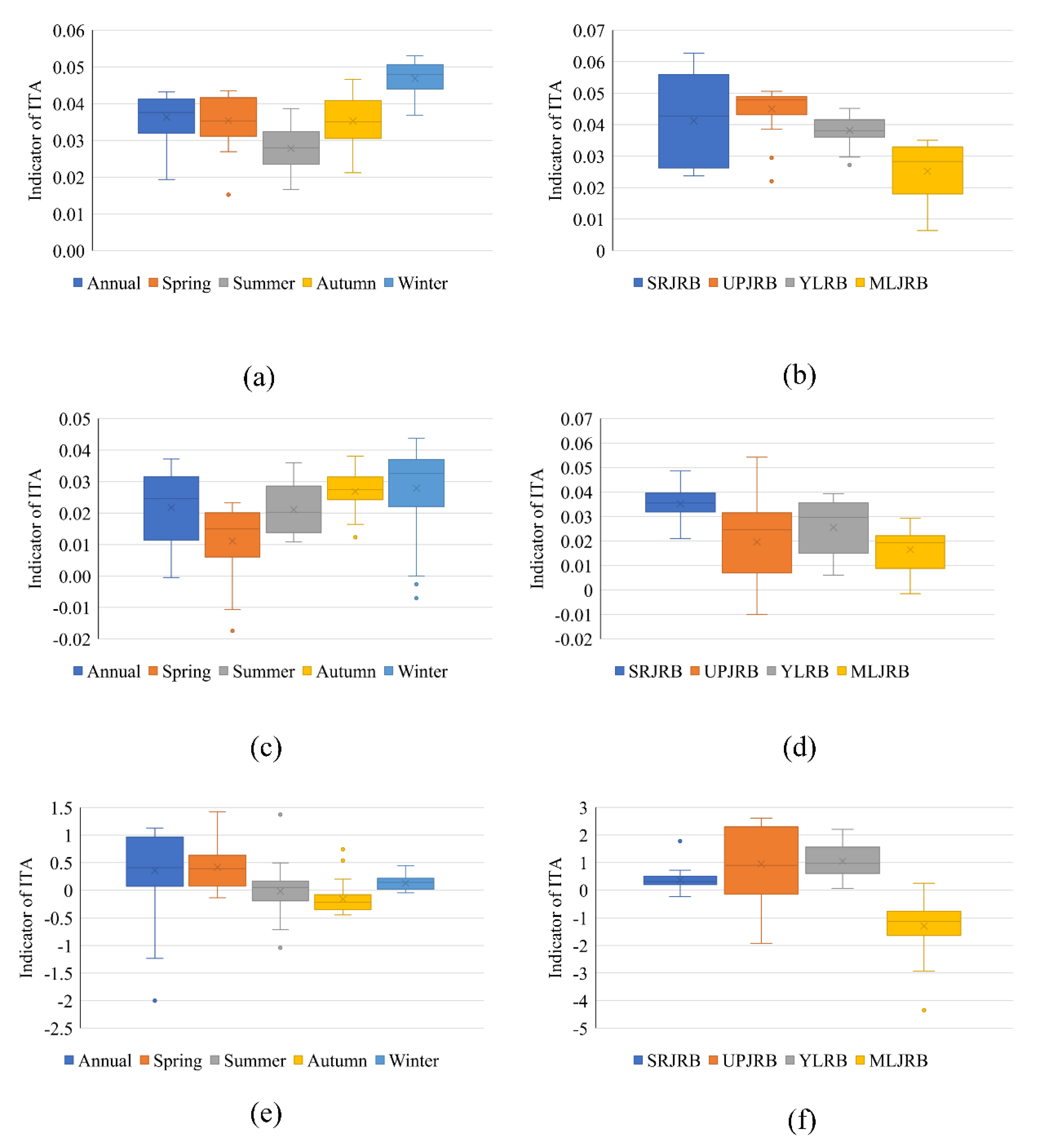
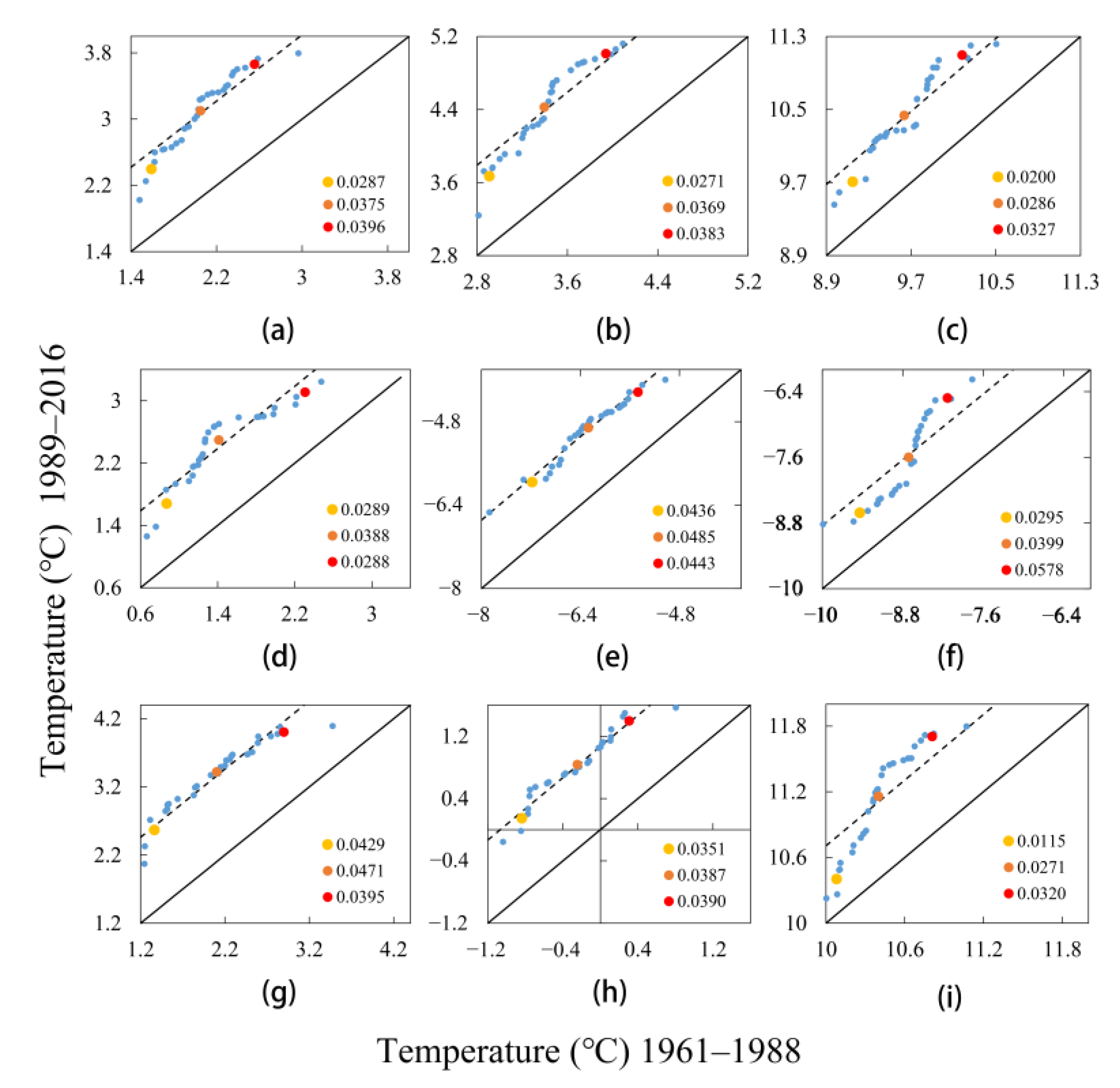
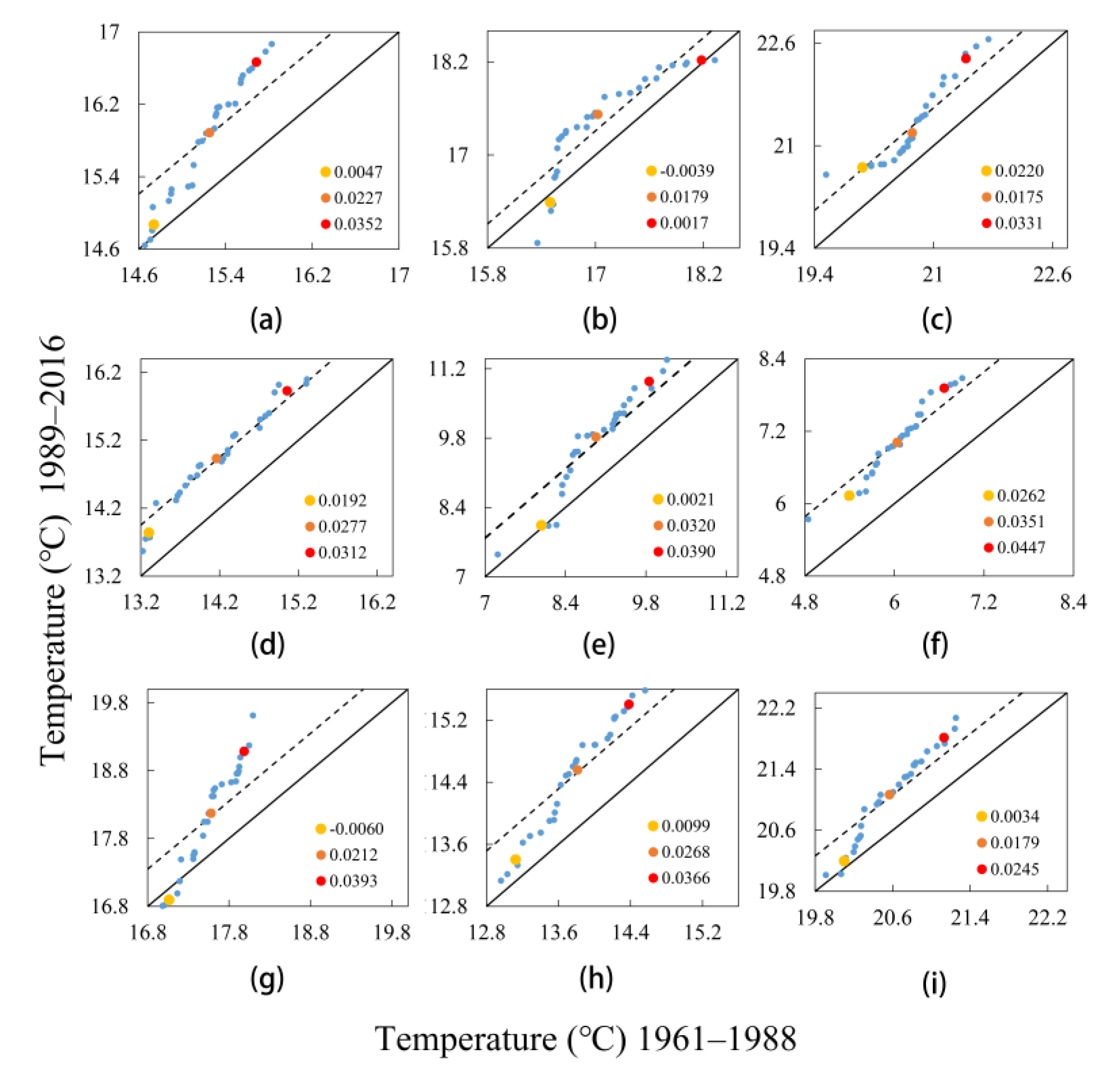
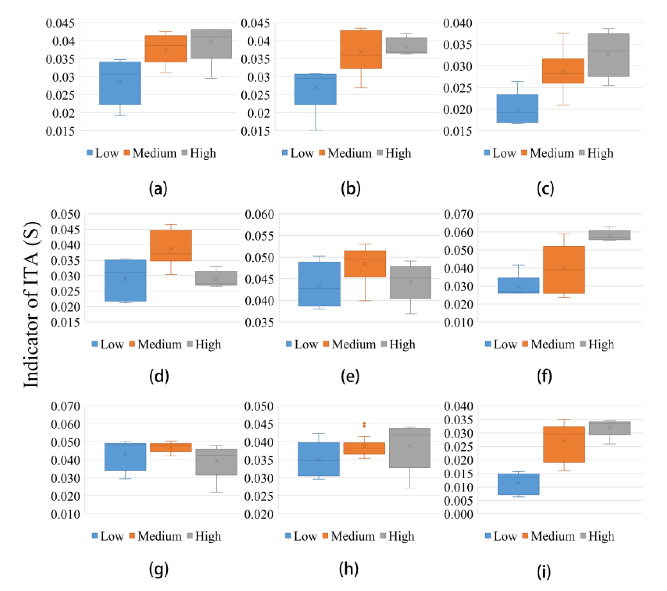
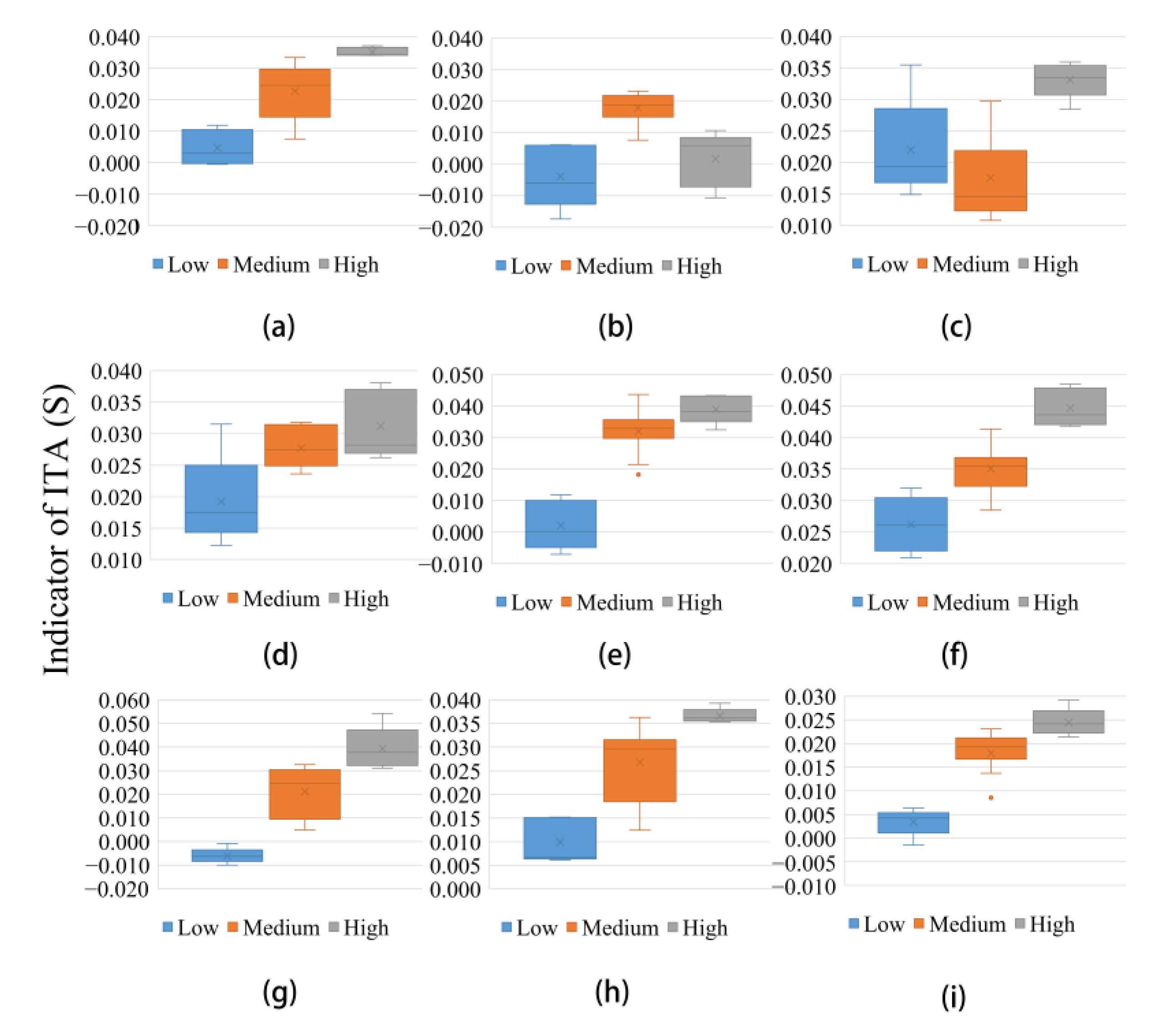
The trends in annual Tmin and Tmax detected by MK and TSA are summarized in Table 2, and the average value of the ITA is shown in Table 3, whereas the median value of the ITA is shown in Figure 4. The slope (S) values calculated by the ITA show increasing trends for the annual Tmin and Tmax at a 99% confidence level in the JRB, which is consistent with the statistic index Z calculated by the MK index b in the TSA. However, according to Figure 5a and Figure 6a, which represent the indicators of the ITA using average values, as well as Figure 7a and Figure 8a, which represent the median value, the trends in the annual Tmin across the three categories ranged from 0.0287 to 0.0396 °C/year, while the trends in the different categories of Tmax were more distinct. A slight increase of 0.0047 °C/year was detected for the “low” Tmax category, whereas a strong upward trend of 0.0352 °C/year was found for the “high” category. Furthermore, the indicators of the ITA, MK, and TSA based on Tmin were larger than those of Tmax. The ITA graphical results further show that this conclusion is applicable to all three categories for both average values (Figure 5 and Figure 6) and median values (Figure 7 and Figure 8). Moreover, the temperature variation range can be estimated by removing the “low” category of Tmin from the “high” category of Tmax. Therefore, the ITA results also indicate that the temperature variation range decreased because the increasing speed of the “low” Tmin category was faster than that of the “high” Tmax category.
For seasonal air temperature, the indicators calculated by three trend analysis methods (Table 2 and Table 3), and the ITA graphs (Figure 4, Figure 5, Figure 6, Figure 7 and Figure 8) indicate that both Tmin and Tmax had significant increasing trends at a 99% confidence level in the JRB for all seasons, with the temperature in winter showing a more obvious increase compared with the other seasons. However, further inspection of the ITA results revealed distinct trends for different categories in different seasons. The trends in spring and winter Tmax were non-monotonically increasing, while the “low” categories of the spring Tmax showed a slightly decreasing trend. Besides, except for the autumn Tmin, the increasing trend of the “high” categories was more obvious than that of the “low” and “medium” categories. In addition, it is noteworthy that the variation range in the summer and autumn temperatures tended to decrease, whereas the opposite was true for the spring and winter temperatures.
The increasing trends for the annual Tmin and Tmax in the JRB are supported by previous studies. A strong warming in China over the past five decades was reported by Piao et al. [6] based on continuous measurements from 412 meteorological stations; the annual mean temperature increased at a rate of 0.27 °C/decade from 1960 to 2005. Su et al. [17] noted that the seasonal mean maximum temperature in the Yangtze River basin showed a slight decrease in summer, but that the mean minimum temperature increased for all seasons. Guan et al. [57] showed that during 1960–2012, the annual mean values of the daily minimum and maximum temperature increased throughout the YRB. Cui et al. [35] linked climate warming to increased spring and winter temperatures in the YRB. Ren et al. [58] pointed out that the annual mean surface air temperature over the Hindu Kush Himalayan (HKH) region significantly increased from 1901 to 2014. Another study, conducted by Kang et al. [59], reconstructed the 70-year history of summer air temperatures based on an ice core record in the source region of the Yangtze River, and their results showed that summer temperatures have dramatically increased since the 1990s. In addition, based on tree rings, Liang et al. [60] reconstructed the mean summer temperature in southeastern Tibet during the past 242 years and compared it with instrumental records from 1961 onward. Their results indicated that southeastern Tibet has recently been warming (in a long-term context), and that the last decade was the warmest period since 1765. More specifically, Wang and Zhang [36] analyzed the trends of annual and seasonal temperatures in the JRB and showed that the mean temperature has an increasing trend; this finding was supported by Li et al. [38]. This study adds to the body of research by revealing the hidden trends in three categories of annual and seasonal Tmin and Tmax.
3.1.2. Spatial Patterns of Trends
The indicators of the MK, TSA, and ITA methods based on sub-basin scale annual mean air temperature time series are shown in Table 2 and Table 3, and the graphical results of ITA are shown in Figure 4, Figure 5, Figure 6, Figure 7 and Figure 8. The indicators of three methods show significant increasing trends at αv = 0.01 for all sub-basins. Most of the results calculated by ITA based on the sub-basin time series were beyond the 1:1 line, implying overall increasing trends for all sub-basins. However, the trends in different temperature categories were distinct in the separate sub-basins. The trends in the annual Tmax in UPJRB and MLJRB non-monotonically increased, whereas Tmin increased monotonically in the four sub-basins. The increasing trend of the three categories of Tmin in UPJRB and YLRB were similar, but for Tmin in SRJRB and MLJRB, as well as Tmax in the four sub-basins, the increasing trend of the “high” categories was much larger than that in the “low” categories. The results show that more attention should be paid to the Tmin change in the YLRB. As shown in Figure 5h, the annual minimum temperature changed from negative to positive. This may potentially affect the hydrological cycle; for example, it could change the relationship between precipitation and runoff, which could trigger serious consequences. Moreover, based on the trends in the “low” categories of Tmin and the “high” categories of Tmax, the temperature variation range tended to narrow in UPJRB and YLRB, whereas the opposite was true in the SRJRB and MLJRB.
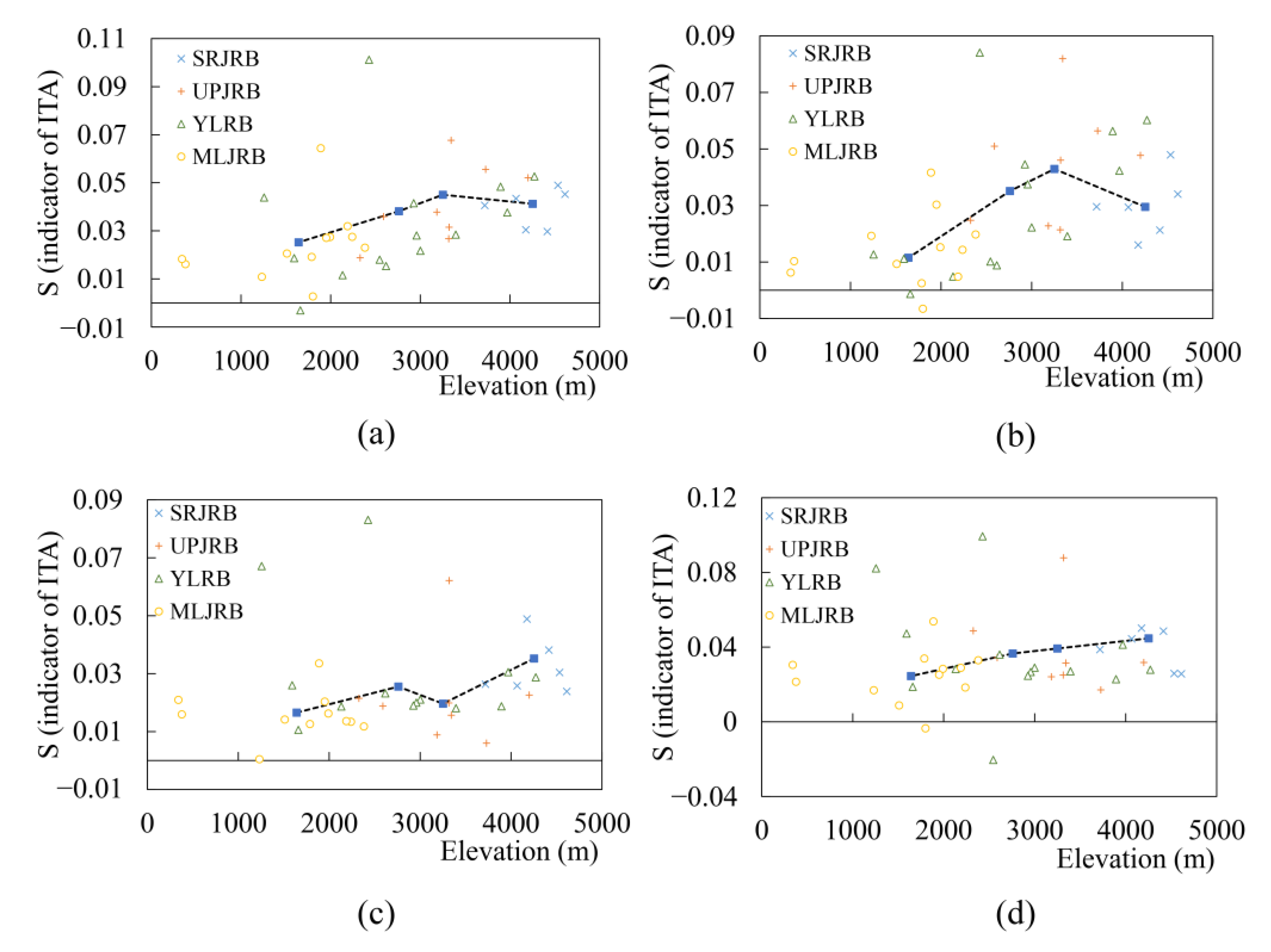
The results calculated by ITA (Table 3 and Figure 4) also show that the MLJRB has the lowest increase, whereas the slope of the SRJRB was the largest. As shown in Table 1, the elevation of the observed stations varies from 341 to 4612 m. Thus, to analyze the impact of elevation on temperature trends, scatter plots were introduced to show S (the indicator of the ITA) versus elevation based on the annual temperature time series of the 40 stations. In addition, the Tmin and Tmax time series, as well as the “low” categories of Tmin and the “high” categories of Tmax were taken into consideration (Figure 9). Overall, the results indicate that high elevation areas showed more increasing trends in both Tmin and Tmax than flat areas. The combination of snow-albedo feedbacks and effects of cloud-radiation closely correlate with this phenomenon [35]. Figure 9 also shows that the trend in the “high” category of Tmax increased consistently regardless of elevation; however, the increasing rate in the “low” category of Tmin reached its maximum value at an elevation near 3300 m. Where the elevation is higher than 3300 m, the “low” category of Tmin, as well as Tmin, warms more slowly with increasing elevation levels. This is consistent with the findings of Du et al. [43], who, based on mean temperatures, pointed out that climate warming rates are decreasing with increasing elevation levels in parts of the Tibet area. Therefore, our results confirm that elevation is an important factor in temperature trend differences in the JRB, where the impact of elevation on the trends of “low” Tmin category is more complex, as compared with the “high” Tmax category.
3.1.3. Potential Impacts of Temperature Trends
The increasing trends of Tmin and Tmax have potential implications for human health and the social and economic development of the JRB. Previous studies reported that the spatiotemporal changes of Tmin and Tmax have a significant impact on temperature extremes (including frequency, intensity, and duration) worldwide, which will further affect human health and cause outbreaks of infectious diseases [61]. Moreover, the observed changes in Tmin and Tmax can change water conditions and other environmental factors, resulting in a considerable impact on water supplies and natural ecosystems [4]. For instance, an increase in temperature in the SRJRB can accelerate the melting process for snow and glaciers, which results in increased river flow and more water for domestic purposes in downstream regions [36]. However, excessive melting may also cause spring floods that will bring new challenges for flood control. As glaciers continuously retreat, river flows may decrease, causing water shortages and associated serious environmental and social problems. Moreover, increases in Tmin and Tmax play a vital role in agriculture and food security. Increasing temperatures have positive impacts on reducing the growing season, allowing both earlier planting and later harvesting [55]; however, they also pose potential risks to the agricultural sector. For example, temperature increases directly affect the water requirements of crops [62] and can have an indirect impact on soil erosion [63]. Moreover, increases in temperature can expand the ranges of pests and diseases [6].
3.2. Precipitation Trends
3.2.1. Annual and Seasonal Trends
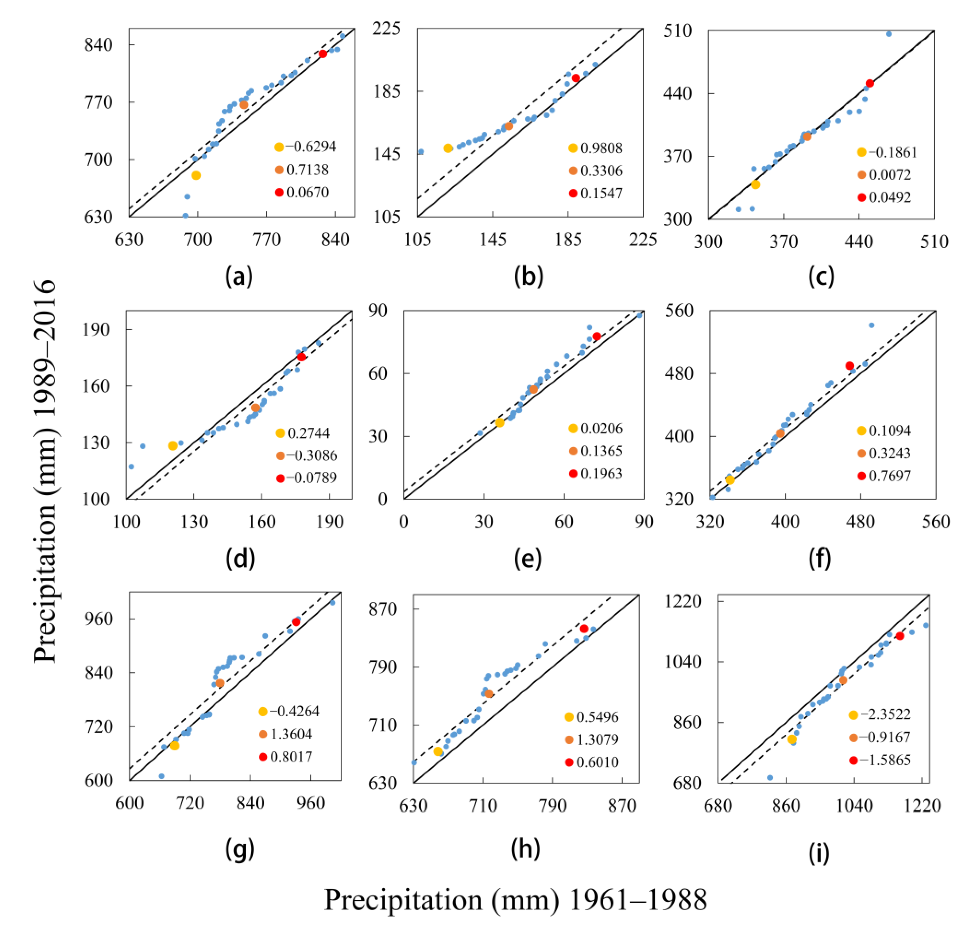
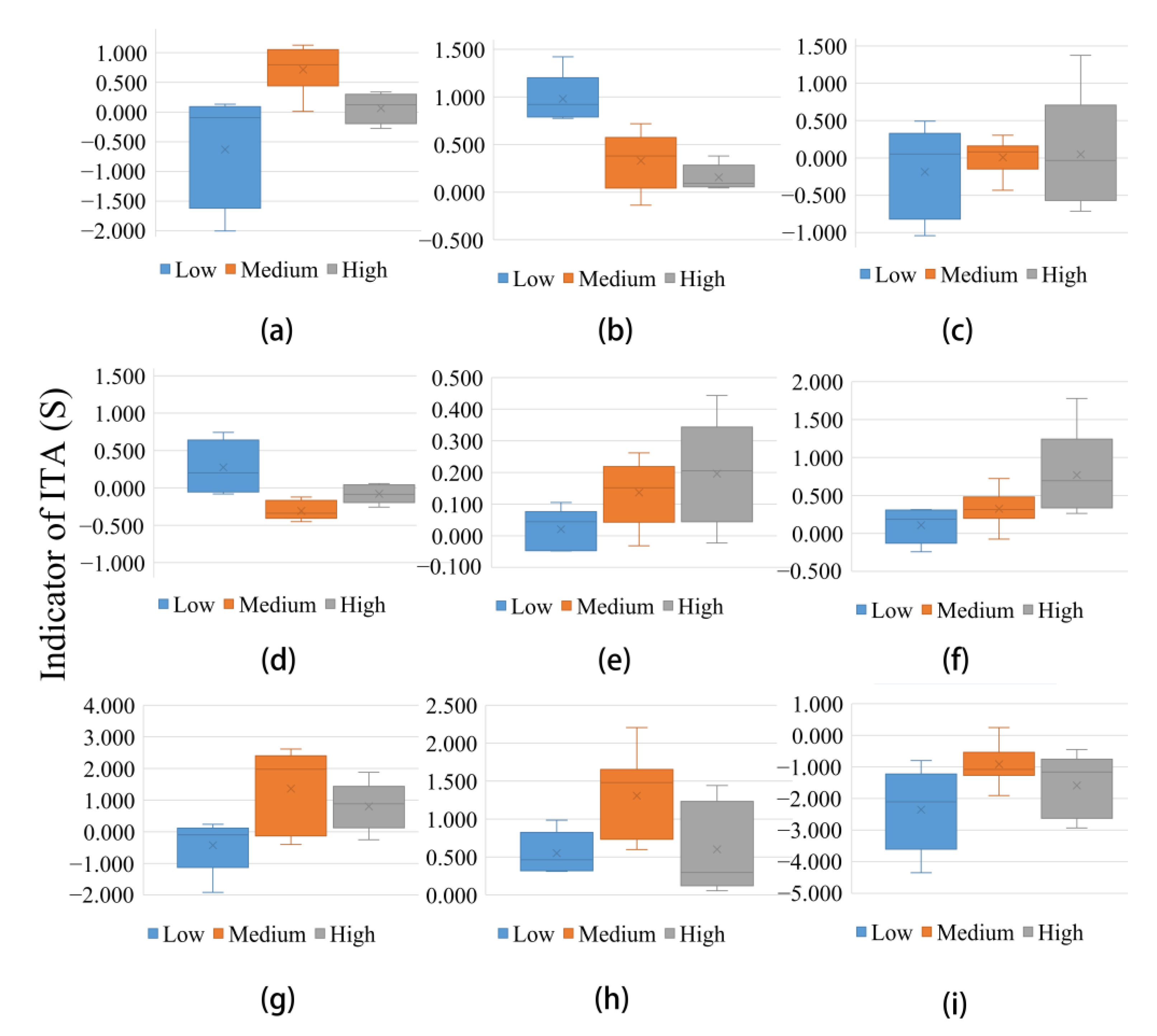
The trend in the annual precipitation in the JRB was detected using three methods, as summarized in Table 2 and Table 3 and Figure 4. According to the ITA, annual precipitation showed an increasing trend in the JRB. The annual precipitation trends in the three categories (low, medium, and high) detected by the ITA are shown in Figure 10a and Figure 11a. The results show that most points were beyond the 1:1 line, implying a non-monotonic increasing trend in annual precipitation in the JRB. However, for the “low” category, we observed a decreasing trend (−0.6294 mm/year), while for the “medium” precipitation category there was an increasing trend (0.7138 mm/year); both trends were significant at a 99% confidence level. For the “high” category, we observed no significant trends, with all points falling along the no trend line.
For seasonal precipitation (Table 2 and Table 3 and Figure 4), although all methods agreed that precipitation in summer had a nonsignificant decreasing trend, the ITA methods showed significant increasing trends at a 99% confidence level in spring, autumn, and winter. Figure 10 and Figure 11 depict the results for the three seasonal precipitation categories that were calculated using the ITA method. For the “low” category of summer precipitation, we observed a decreasing trend, whereas a significant increasing trend was found for spring and autumn precipitation. For the “high” category, there was no significant trend in summer and autumn precipitation; however, a significant increasing trend was found in spring and winter precipitation.
According to the Intergovernmental Panel on Climate Change (IPCC), precipitation has increased since 1951 over mid-latitude land areas in the Northern Hemisphere [1]. The conclusions drawn by Ren et al. [34] indicate that CMIP5 projected a continuing and stronger global precipitation trend in the 21st century. However, according to Anagnostopoulos et al. [64] and Koutsoyiannis et al. [65], the climate model projections performed poorly compared with the observed precipitation levels, and the inability to reproduce climate observations implies a structural uncertainty within climate models. In China, there was no significant (at a 95% confidence level) trend in the annual country-wide average precipitation from 1960, but obvious regional differences were detected [6]. Cui et al. [35] found that annual precipitation increased insignificantly (95% confidence level) at a rate of approximately 12.02 mm/decade in the YRB from 1960 to 2015. Ren et al. [34] analyzed the long-term changes in precipitation in the HKH region from 1901 to 2014 and concluded that annual precipitation decreased slightly during the study period. However, the annual precipitation trend showed a statistically significant increase from 1961 to 2013 in the HKH region. More specifically, Wang et al. [37] concluded that there was a nonsignificant (at the 95% confidence level) increasing trend in annual precipitation in the JRB, and that autumn precipitation had an insignificant decreasing trend, whereas other seasons showed an increasing trend. Compared with the traditional methods (Table 2), the findings based on the ITA (Table 3) in this study indicate that in the JRB, annual, spring, and winter precipitation had an increasing trend from 1961 to 2016, whereas the precipitation during autumn showed a decreasing trend.
Many researchers have compared the ITA method with traditional methods, including MK, and the ITA has proven to be a viable and effective means of analyzing trends [26,27,28,29,30,31]. Together with the significance test proposed by Sen [24], the ITA method can analyze hidden trends in rainfall series that cannot be detected using traditional methods. For example, Li et al. [66] showed that the ITA was able to successfully detect 138 significant trends (p < 0.01 or p < 0.05), including 89 time series that could not be detected when using the linear regression analysis (LRA) or MK methods. For 70 annual and seasonal precipitation series in the Yangtze delta, Wang et al. [10] detected significant trends in 31 time series using the MK method, whereas 61 time series exhibited significant trends using the ITA method. In addition, this study further revealed that the “low” annual precipitation category had a significant decreasing trend, while the “high” categories of spring precipitation had a significant increasing trend.
3.2.2. Spatial Patterns of Precipitation Trends
Indicators based on the sub-basin scale precipitation time series for the MK, TSA, and ITA methods are shown in Table 2 and Figure 3, Figure 4, Figure 10 and Figure 11. Except for the MLJRB, the annual precipitation in the sub-basins showed an increasing trend. ITA showed a significant increasing trend at the 99% confidence level in the four sub-basins, whereas the MK method treated the precipitation trend in the YLRB as significant at the 95% confidence level. Further inspection of the ITA graphical results revealed different tendencies of precipitation in different categories. As shown in Figure 10 and Figure 11, the “low” categories of precipitation in the UPJRB and MLJRB showed significant decreasing trends, and except for the MLJRB, the “high” categories of precipitation in the sub-basins all showed significant increasing trends.
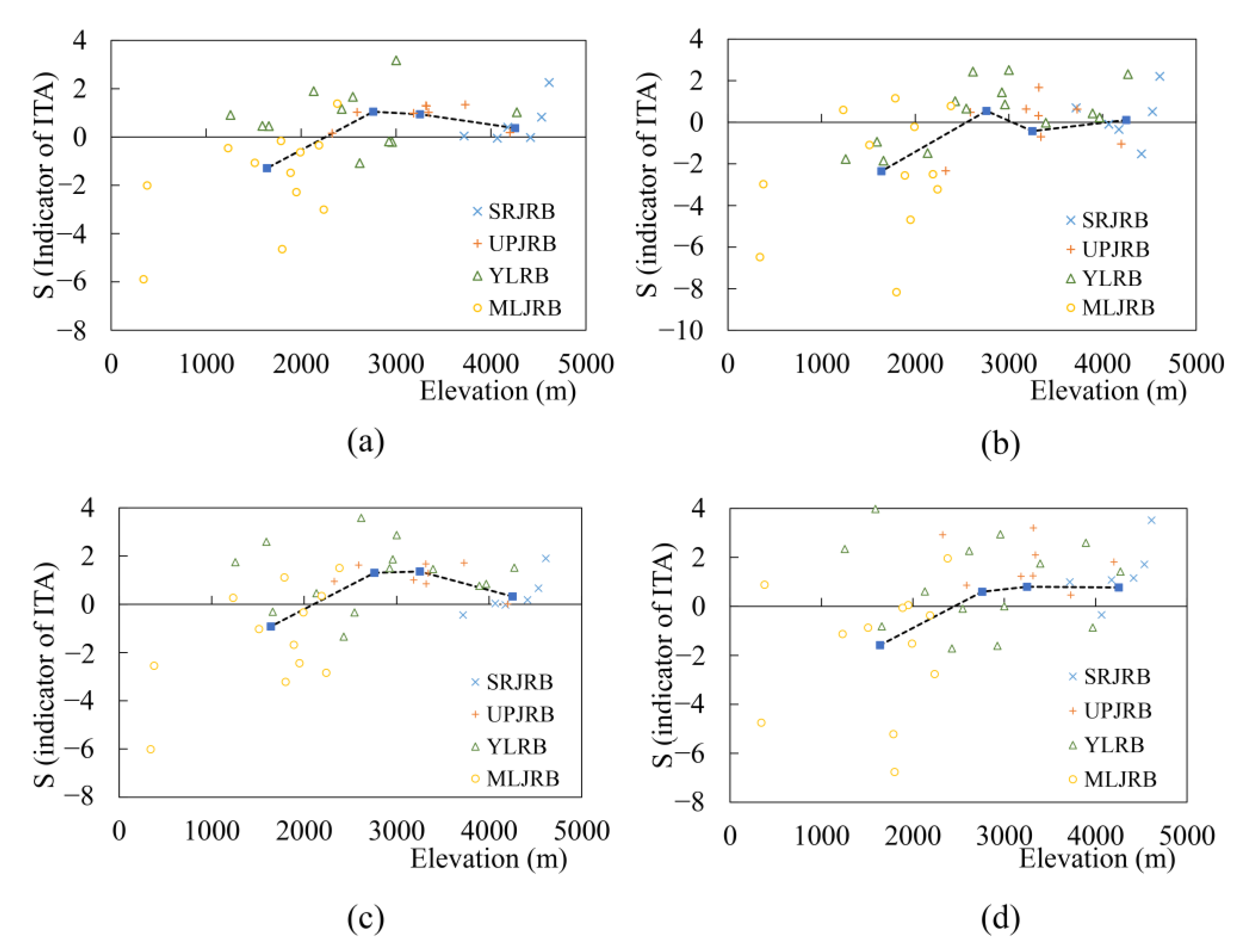
Scatter plots of S (indicator for ITA) versus elevation based on the annual precipitation time series of the 40 stations reveal the impact of elevation on the precipitation trends. Figure 12a shows that the largest increase in annual precipitation was at an elevation of ~2500 m. With decreasing elevation, precipitation trends also decreased; however, with increasing elevation, precipitation trends weakened. The three precipitation categories (low, medium, and high; Figure 12b–d, respectively) partly explain the reason for this and reveal another interesting phenomenon. Figure 12 shows that annual precipitation had a significant decreasing trend for all three categories where the elevation was <2000 m. However, for the “low” precipitation category, the significant increasing trend mainly occurred for elevations around 2500 m, for the “medium” category, the significant increasing trend occurred up to 3000 m, and for the “high” category, the increasing trend occurred for elevations >2000 m. Thus, the trends in annual precipitation are related to elevation in the JRB. This conclusion contradicts the finding in the Hengduan Mountains [67]; however, similar conclusions were observed in the China–Pakistan economic corridor by Ullah et al. [68]. Although some experts reported that this phenomenon could be the result of orographic and physiographic dynamics or shifting weather systems [69], the reasons behind the precipitation trend and elevation relationship still need to be explored [68].
3.2.3. Potential Impact of Precipitation Trends
The annual precipitation in the JRB showed nonsignificant changes; however, considerable attention should be paid to seasonal precipitation trends and the trends of the sub-basins. For instance, the increase in precipitation for the “high” category in spring may cause more floods and associated geological disasters. On the other hand, the decreasing trend of precipitation in the “low” category in summer will bring new challenges for agricultural production in the JRB. Moreover, the increasing trends in precipitation in the SRJRB and the YLRB, especially for the “high” category, may increase the intensity of floods and landslides. The increases in the “medium” category in these two sub-basins may provide more water resources to the catchment of the South to North Water Transfer Western Route Project [70]. However, the decreasing trends in the “low” precipitation category in the MLJRB, coupled with an increasing population and the development of agriculture and industry, will widen the gap between water supply and water demand [6].
3.3. Relationship between Air Temperature and Precipitation
To evaluate the possible relationships between minimum and maximum temperature and precipitation, correlations were evaluated using the Pearson’s correlation test (Figure 13 and Figure 14).
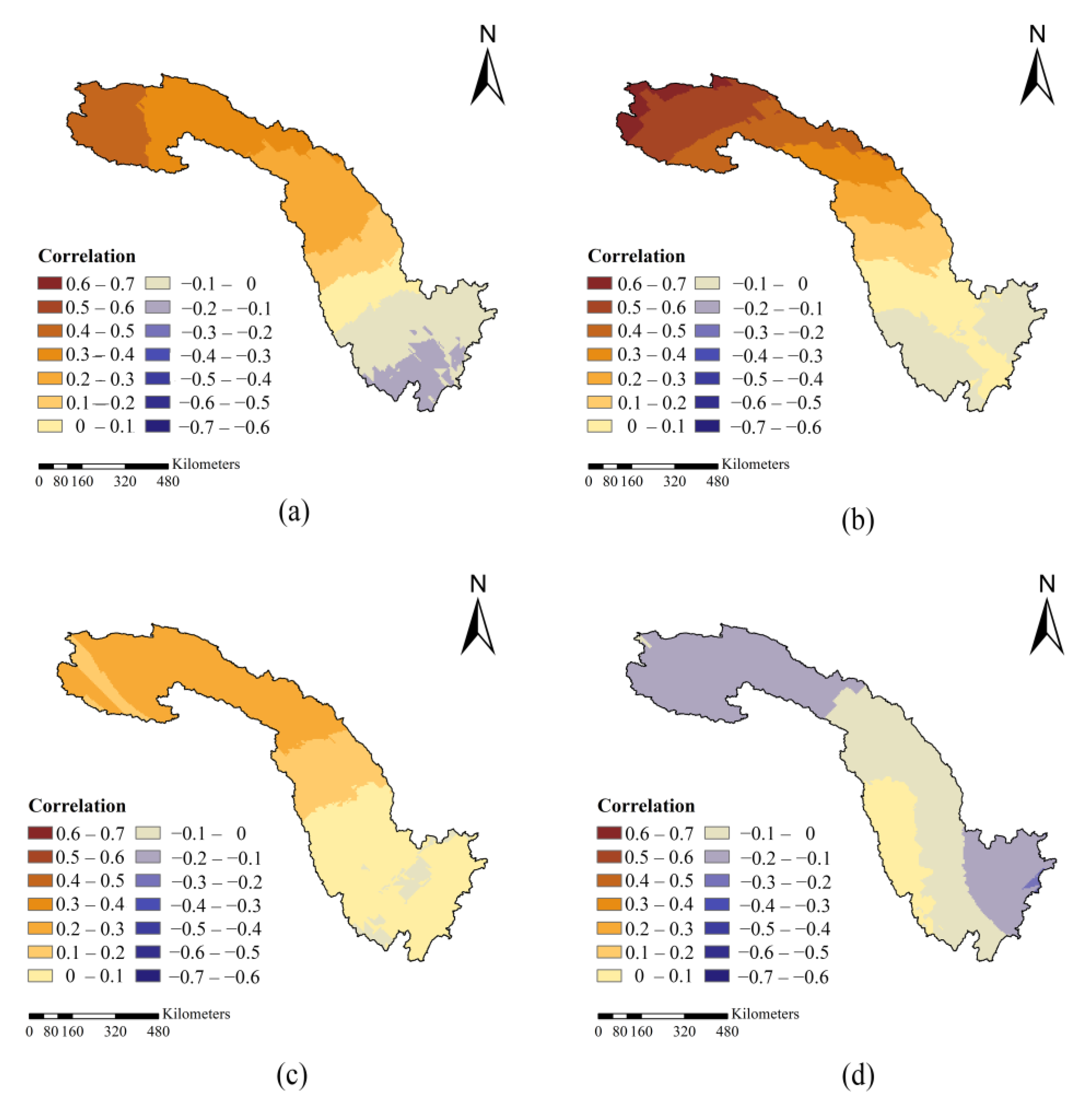
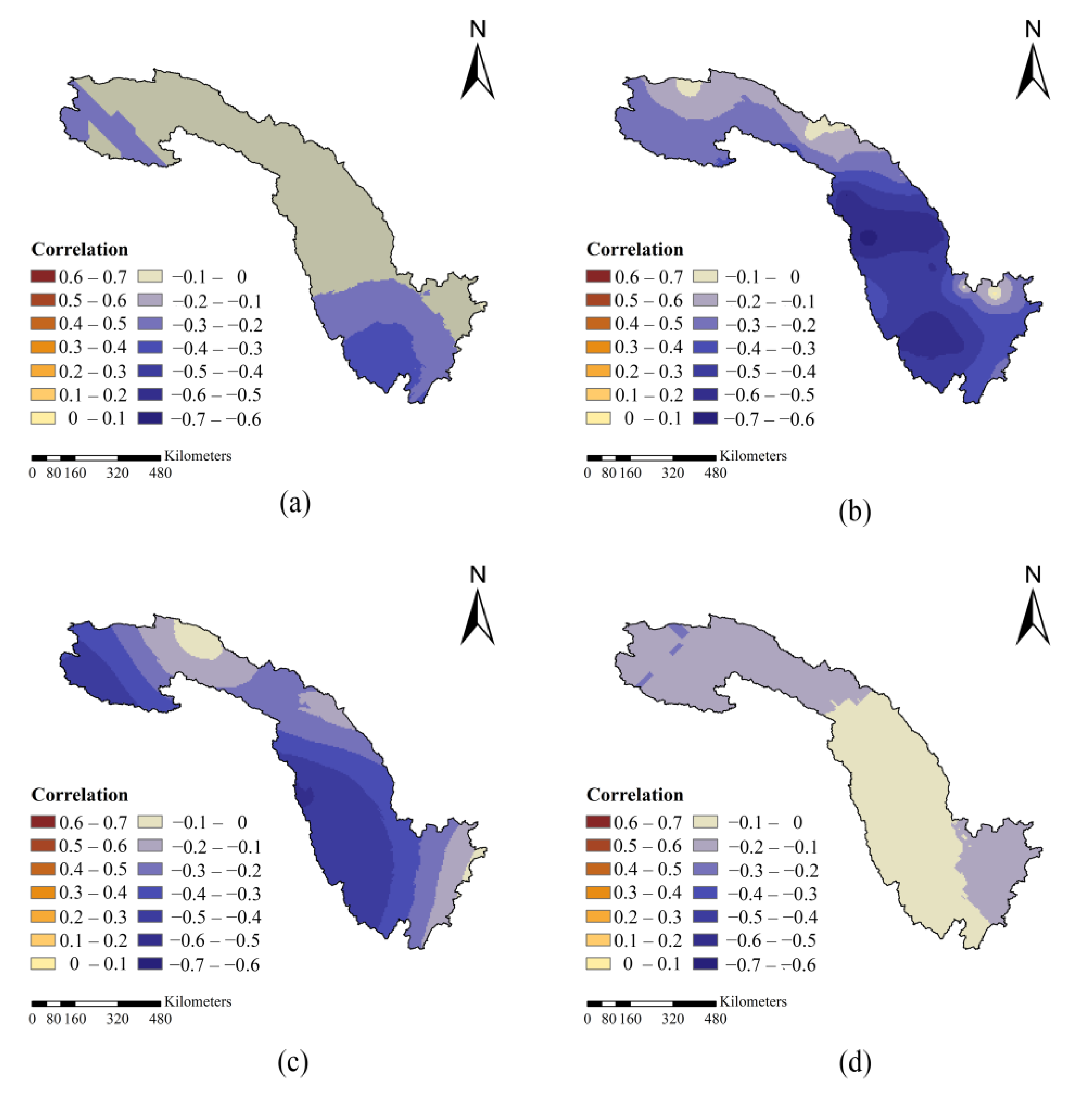
The correlations between precipitation and minimum temperature showed obvious spatial differences in each season, with values of −0.13 to 0.47, −0.13 to 0.64, −0.03 to 0.30, and −0.22 to 0.06 during spring, summer, autumn, and winter, respectively. A strong positive correlation was observed in the northwestern part of the JRB in spring, summer, and autumn, with a decreasing gradient from northwestern to southeastern areas. Although certain regions showed positive correlations in summer, negative correlations between precipitation and maximum temperature were observed year-round. These correlations range from −0.45 to −0.19 (spring), −0.71 to 0.05 (summer), −0.52 to −0.06 (autumn), and −0.31 to −0.11 (winter). A strong negative correlation existed in the southern (spring) and central and southwestern (summer and autumn) areas.
The results of the correlation between temperature and precipitation can also be found in previous studies. Trenberth and Shea [71] presented negative correlations between temperature and precipitation in summer over land, with wet conditions favoring cooler temperatures and dry conditions favoring more sunshine. According to Isaac and Stuart [72], the correlation between temperature and precipitation at west coast sites in Northern Canada reversed with season, and more precipitation falls during warm winters and cool summers in and downwind of the Rocky Mountains; the correlation is consistent year-round, and more precipitation occurs when the temperature is colder. A seasonal correlation in eastern India was detected by Sharma et al. [2], with the relationship between maximum temperature and precipitation dominated by a negative correlation.
For the SRJRB, precipitation and the minimum temperature showed a strong positive correlation in spring and summer, which indicates an increasing trend in precipitation and a resulting increase in flood risk. However, for the MLJRB, strong negative correlations between precipitation and maximum temperature in spring, summer, and autumn indicate a reduction in precipitation accompanied by higher temperatures that will affect the water requirements for crop growth, drinking, and other domestic purposes [37]. For example, in the summer of 2013, the severe drought caused by a persistent heatwave and lack of rain brought a direct economic loss of more than 8 billion USD in China [57].
4. Conclusions
This study applied the ITA method to evaluate trends in the annual and seasonal minimum temperature (Tmin), maximum temperature (Tmax), and precipitation in the JRB. Furthermore, the impact of elevation on the spatial patterns of trends and the correlations between precipitation and temperature were analyzed. The main conclusions follow.
- (1)
- Annual and seasonal temperatures showed significant increasing trends over the JRB at a 99% confidence level. Subcategory (low, medium, and high) results indicate that the increasing trends of Tmin were consistent, whereas those of the “high” category of Tmax were more obvious than for the other categories. In addition, the variation ranges of annual, summer, and autumn temperatures tended to decrease, whereas the opposite was true for spring and winter. Sub-basin results indicate that high elevation areas showed a larger increase in Tmin than lower elevation areas.
- (2)
- The annual precipitation showed an increasing trend in the JRB according to the ITA; however, a significant decreasing trend was present in the “low” categories at a 99% confidence level, whereas no trend occurred in the “high” precipitation categories. There were no consistent trends for seasonal precipitation, and the “low” category of summer precipitation showed a decreasing trend, whereas there was an increasing trend for the “high” category of spring precipitation. In terms of spatial patterns, the precipitation in the MLJRB showed a decreasing trend, whereas other sub-basins showed an increasing trend. Further analyses show that the impact of elevation on different categories of precipitation was distinctive where the elevation was >2000 m.
- (3)
- The present study additionally examined the correlation between temperature and precipitation in the JRB. For the SRJRB, strong positive correlations occurred between precipitation and the minimum temperature in spring, summer, and autumn, whereas the opposite dynamic was observed for the relationship between precipitation and the maximum temperature in the MLJRB. The combined change in temperature and precipitation will pose new challenges for water resource management, agriculture, and economic development in the JRB.
The results of this study provide a resource for drought and flood disaster control, agricultural and water resource management, ecological protection, social development, future water resources design, and future climate prediction in the study area. The trend analysis in this study was based on instrumental observations in the last 56 years. It would be interesting to explore whether such a trend is occurring outside the envelope of variability observed in the geologic record. Much more work is needed to answer this challenging question and it is a little out of the scope of this study. However, the surface temperature at hemispheric and global scales for the last 2000 years showed that the recent warmth (around the last 60 years) appeared to be anomalies for at least the past 1300 years [73]. That is to say, this warming trend is outside of climate variability in the last 1300 years. Moreover, it will be necessary to conduct further research to provide a comprehensive view of climate change in the JRB, including the impacts of other orographic and physiographic factors (except for elevation) on the connections between trend and large-scale climate anomalies [74].
Author Contributions
Conceptualization, W.J. and Z.D.; methodology, Q.M.; software, W.J.; validation, R.S., G.F., and Z.D.; investigation, W.J.; resources, Z.D.; data curation, Q.W.; writing—original draft preparation, W.J.; writing—review and editing, W.J., R.S., and G.F.; visualization, W.J. and Q.M.; supervision, Z.D., R.S., and G.F.; funding acquisition, Z.D. All authors have read and agreed to the published version of the manuscript.
Funding
This research was funded by the National Key Research and Development Plan of China, grant number 2016YFC0402209.
Conflicts of Interest
The authors declare no conflict of interest
Appendix A
Monthly maximum and minimum air temperature data and monthly precipitation data were obtained from the China Meteorological Administration (http://data.cma.cn, accessed on 15 September 2020). Annual and seasonal air temperature data and precipitation data in the JRB and four sub-basins is available from: 10.17632/5hpn8jcrbt.1 (accessed on 15 September 2020).
References
- IPCC. Climate Change 2014: Synthesis Report. Contribution of Working Groups I, II and III to the Fifth Assessment Report of the Intergovernmental Panel on Climate Change; Core Writing Team, Pachauri, R.K., Meyer, L.A., Eds.; Cambridge University Press: Cambridge, UK, 2014. [Google Scholar] [CrossRef]
- Sharma, C.S.; Panda, S.N.; Pradhan, R.P.; Singh, A.; Kawamura, A. Precipitation and temperature changes in eastern India by multiple trend detection methods. Atmos. Res. 2016, 180, 211–225. [Google Scholar] [CrossRef]
- Allen, M.R.; Ingram, W.J. Constraints on future changes in climate and the hydrologic cycle. Nature 2002, 419, 224–232. [Google Scholar] [CrossRef] [PubMed]
- Barnett, T.; Adam, J.; Lettenmaier, D. Potential impacts of a warming climate on water availability in snow-dominated regions. Nature 2005, 438, 303–309. [Google Scholar] [CrossRef] [PubMed]
- Oki, T.; Kanae, S. Global Hydrological Cycles and World Water Resources. Science 2006, 313, 1068–1072. [Google Scholar] [CrossRef] [Green Version]
- Piao, S.; Ciais, P.; Huang, Y.; Shen, Z.; Peng, S.; Li, J.; Zhou, L.; Liu, H.; Ma, Y.; Ding, Y.; et al. The impacts of climate change on water resources and agriculture in China. Nature 2010, 467, 43–51. [Google Scholar] [CrossRef]
- Bo, L.; Qi, H.; Wang, W.; Zeng, X.; Zhai, J. Variation of actual evapotranspiration and its impact on regional water resources in the Upper Reaches of the Yangtze River. Quat. Int. 2011, 244, 185–193. [Google Scholar] [CrossRef]
- Zhang, Q.; Xu, C.Y.; Zhang, Z.; Chen, Y.D.; Liu, C.L.; Lin, H. Spatial and temporal variability of precipitation maxima during 1960–2005 in the Yangtze River basin and possible association with large-scale circulation. J. Hydrol. 2008, 353, 215–227. [Google Scholar] [CrossRef]
- Şen, Z. Partial trend identification by change-point successive average methodology (SAM). J. Hydrol. 2019, 571, 288–299. [Google Scholar] [CrossRef]
- Wang, Y.; Xu, Y.; Tabari, H.; Wang, J.; Wang, Q.; Song, S.; Hu, Z. Innovative trend analysis of annual and seasonal rainfall in the Yangtze River Delta, eastern China. Atmos. Res. 2020, 231, 104673. [Google Scholar] [CrossRef]
- Mann, H.B. Nonparametric Tests against Trend. Econometrica 1945, 13, 245–259. [Google Scholar] [CrossRef]
- Kendall, M.G. Rank Correlation Methods; Griffin: Oxford, UK, 1975; Available online: https://psycnet.apa.org/record/1948-15040-000 (accessed on 15 September 2020).
- Arnone, E.; Pumo, D.; Viola, F.; Noto, L.V. Rainfall Statistic Changes in Sicily. Hydrol. Earth Syst. Sci. 2013, 17, 2449–2458. [Google Scholar] [CrossRef] [Green Version]
- Van Loon, A.F.; Laaha, G. Hydrological drought severity explained by climate and catchment characteristics. J. Hydrol. 2015, 526, 3–14. [Google Scholar] [CrossRef] [Green Version]
- Sen, P.K. Estimates of the Regression Coefficient Based on Kendall’s Tau. J. Am. Stat. Assoc. 1968, 63, 1379–1389. [Google Scholar] [CrossRef]
- Gocic, M.; Trajkovic, S. Analysis of changes in meteorological variables using Mann-Kendall and Sen’s slope estimator statistical tests in Serbia. Glob. Planet. Chang. 2013, 100, 172–182. [Google Scholar] [CrossRef]
- Su, B.D.; Jiang, T.; Jin, W.B. Recent trends in observed temperature and precipitation extremes in the Yangtze River basin, China. Theor. Appl. Climatol. 2006, 83, 139–151. [Google Scholar] [CrossRef]
- Chowdhury, R.K.; Beecham, S.; Boland, J.; Piantadosi, J. Understanding South Australian rainfall trends and step changes. Int. J. Climatol. 2015, 35, 348–360. [Google Scholar] [CrossRef]
- Jones, J.R.; Schwartz, J.S.; Ellis, K.N.; Hathaway, J.M.; Jawdy, C.M. Temporal variability of precipitation in the Upper Tennessee Valley. J. Hydrol. Reg. Stud. 2015, 3, 125–138. [Google Scholar] [CrossRef] [Green Version]
- Sabzevari, A.A.; Zarenistanak, M.; Tabari, H.; Moghimi, S. Evaluation of precipitation and river discharge variations over southwestern Iran during recent decades. J. Earth. Syst. Sci. 2015, 124, 335–352. [Google Scholar] [CrossRef]
- Wu, H.; Qian, H. Innovative trend analysis of annual and seasonal rainfall and extreme values in Shaanxi, China, since the 1950s. Int. J. Climatol. 2017, 37, 2582–2592. [Google Scholar] [CrossRef]
- Şen, Z. Innovative Trend Analysis Methodology. J. Hydrol. Eng. 2012, 17, 1042–1046. [Google Scholar] [CrossRef]
- Şen, Z. Trend Identification Simulation and Application. J. Hydrol. Eng. 2014, 19, 635–642. [Google Scholar] [CrossRef]
- Şen, Z. Innovative trend significance test and applications. Theor. Appl. Climatol. 2017, 127, 939–947. [Google Scholar] [CrossRef]
- Sonali, P.; Kumar, D.N. Review of trend detection methods and their application to detect temperature changes in India. J. Hydrol. 2013, 476, 212–227. [Google Scholar] [CrossRef]
- Kisi, O. An innovative method for trend analysis of monthly pan evaporations. J. Hydrol. 2015, 527, 1123–1129. [Google Scholar] [CrossRef]
- Öztopal, A.; Şen, Z. Innovative Trend Methodology Applications to Precipitation Records in Turkey. Water Resour. Manag. 2017, 31, 727–737. [Google Scholar] [CrossRef]
- Wu, H.; Li, X.; Qian, H. Detection of Anomalies and Changes of Rainfall in the Yellow River Basin, China, through Two Graphical Methods. Water 2018, 10, 15. [Google Scholar] [CrossRef] [Green Version]
- Caloiero, T.; Coscarelli, R.; Ferrari, E. Application of the Innovative Trend Analysis Method for the Trend Analysis of Rainfall Anomalies in Southern Italy. Water Resour. Manag. 2018, 32, 4971–4983. [Google Scholar] [CrossRef]
- Elouissi, A.; Sen, Z.; Habi, M. Algerian rainfall innovative trend analysis and its implications to Macta watershed. Arab. J. Geosci. 2016, 9, 303. [Google Scholar] [CrossRef]
- Güçlü, Y.S. Improved visualization for trend analysis by comparing with classical Mann-Kendall test and ITA. J. Hydrol. 2020, 584, 124674. [Google Scholar] [CrossRef]
- Ji, F.; Wu, Z.; Huang, J.; Chassignet, E.P. Evolution of land surface air temperature trend. Nat. Clim. Chang. 2014, 4, 462–466. [Google Scholar] [CrossRef]
- Nguyen, P.; Thorstensen, A.; Sorooshian, S.; Hsu, K.; Aghakouchak, A.; Ashouri, H.; Tran, H.; Braithwaite, D. Global Precipitation Trends across Spatial Scales Using Satellite Observations. Bull. Amer. Meteor. Soc. 2018, 99, 689–697. [Google Scholar] [CrossRef]
- Ren, L.; Arkin, P.; Smith, T.M.; Shen, S.S. Global precipitation trends in 1900–2005 from a reconstruction and coupled model simulations. J. Geophys. Res. Atmos. 2013, 118, 1679–1689. [Google Scholar] [CrossRef]
- Cui, L.; Wang, L.; Lai, Z.; Tian, Q.; Liu, W.; Li, J. Innovative trend analysis of annual and seasonal air temperature and rainfall in the Yangtze River Basin, China during 1960–2015. J. Atmos. Sol. Terr. Phys. 2017, 164, 48–59. [Google Scholar] [CrossRef]
- Wang, S.; Zhang, X. Long-term trend analysis for temperature in the Jinsha River Basin in China. Theor. Appl. Climatol. 2012, 109, 591–603. [Google Scholar] [CrossRef]
- Wang, S.; Zhang, X.; Liu, Z.; Wang, D. Trend Analysis of Precipitation in the Jinsha River Basin in China. J. Hydrometeorol. 2013, 14, 290–303. [Google Scholar] [CrossRef]
- Li, D.; Lu, X.X.; Yang, X.; Chen, L.; Lin, L. Sediment load responses to climate variation and cascade reservoirs in the Yangtze River: A case study of the Jinsha River. Geomorphology 2018, 322, 41–52. [Google Scholar] [CrossRef]
- Peng, T.; Zhang, C.; Zhou, J.Z. Intra- and Inter-Annual Variability of Hydrometeorological Variables in the Jinsha River Basin, Southwest China. Sustainability 2019, 11, 5142. [Google Scholar] [CrossRef] [Green Version]
- Zhang, P.; Cai, Y.; Yang, W.; Yi, Y.; Yang, Z. Climatic and anthropogenic impacts on water and sediment generation in the middle reach of the Jinsha River Basin. River Res. Appl. 2020, 36, 338–350. [Google Scholar] [CrossRef]
- Aizen, V.B.; Aizen, E.M.; Melack, J.M.; Dozier, J. Climatic and Hydrologic Changes in the Tien Shan, Central Asia. J. Clim. 1997, 10, 1393–1404. [Google Scholar] [CrossRef]
- Li, X.; Wang, L.; Guo, X.; Chen, D. Does summer precipitation trend over and around the Tibetan Plateau depend on elevation? Int. J. Climatol. 2017, 37, 1278–1284. [Google Scholar] [CrossRef]
- Du, M.; Liu, J.; Li, Y.; Zhang, F.; Tang, Y. Are high altitudinal regions warming faster than lower elevations on the Tibetan Plateau? Int. J. Glob. Warm. 2019, 18, 363–384. [Google Scholar] [CrossRef]
- You, Q.; Kang, S.; Pepin, N.; Flügel, W.A.; Yan, Y.; Behrawan, H.; Huang, J. Relationship between temperature trend magnitude, elevation and mean temperature in the Tibetan Plateau from homogenized surface stations and reanalysis data. Glob. Planet. Chang. 2010, 71, 124–133. [Google Scholar] [CrossRef]
- Xu, M.; Kang, S.C.; Wu, H.; Yuan, X. Detection of spatio-temporal variability of air temperature and precipitation based on long-term meteorological station observations over Tianshan Mountains, Central Asia. Atmos. Res. 2018, 203, 141–163. [Google Scholar] [CrossRef]
- Berardy, A.; Chester, M.V. Climate change vulnerability in the food, energy, and water nexus: Concerns for agricultural production in Arizona and its urban export supply. Environ. Res. Lett. 2017, 12, 035004. [Google Scholar] [CrossRef]
- Yao, T.; Thompson, L.; Yang, W.; Gao, Y.; Guo, X.; Yang, X.; Duan, K.; Zhao, H.; Xu, B.; Pu, J.; et al. Different glacier status with atmospheric circulations in Tibetan Plateau and surroundings. Nat. Clim. Change 2012, 2, 663–667. [Google Scholar] [CrossRef]
- Kang, S.; Eltahir, E.A.B. Impact of irrigation on regional climate over Eastern China. Geophys. Res. Lett. 2019, 46, 5499–5505. [Google Scholar] [CrossRef] [Green Version]
- Yin, R.; Xiang, Q. An integrative approach to modeling land-use changes: Multiple facets of agriculture in the Upper Yangtze basin. Sustain. Sci. 2010, 5, 9. [Google Scholar] [CrossRef]
- Chen, Q.; Chen, H.; Wang, J.; Zhao, Y.; Xu, C. Impacts of Climate Change and Land-Use Change on Hydrological Extremes in the Jinsha River Basin. Water 2019, 11, 1398. [Google Scholar] [CrossRef] [Green Version]
- Fu, G.; Charles, S.P.; Yu, J.; Liu, C. Decadal Climatic Variability, Trends, and Future Scenarios for the North China Plain. J. Clim. 2009, 22, 2111–2123. [Google Scholar] [CrossRef]
- Oyler, J.W.; Dobrowski, S.Z.; Ballantyne, A.P.; Klene, A.E.; Running, S.W. Artificial amplification of warming trends across the mountains of the western United States. Geophys. Res. Lett. 2015, 42, 153–161. [Google Scholar] [CrossRef] [Green Version]
- Swed, F.S.; Eisenhart, C. Tables for Testing Randomness of Grouping in a Sequence of Alternatives. Ann. Math. Stat. 1943, 14, 66–87. [Google Scholar] [CrossRef]
- Caloiero, T.; Filice, E.; Coscarelli, R.; Pellicone, G. A Homogeneous Dataset for Rainfall Trend Analysis in the Calabria Region (Southern Italy). Water 2020, 12, 2541. [Google Scholar] [CrossRef]
- Peterson, T.C.; Easterling, D.R.; Karl, T.R.; Groisman, P.; Nicholls, N.; Plummer, N.; Torok, S.; Auer, I.; Boehm, R.; Gullett, D.; et al. Homogeneity adjustments of in situ atmospheric climate data: A review. Int. J. Climatol. 1998, 18, 1493–1517. [Google Scholar] [CrossRef]
- Ullah, S.; You, Q.; Ali, A.; Ullah, W.; Jan, M.A.; Zhang, Y.; Xie, W.; Xie, X. Observed changes in maximum and minimum temperatures over China- Pakistan economic corridor during 1980–2016. Atmos. Res. 2019, 216, 37–51. [Google Scholar] [CrossRef]
- Guan, Y.; Zhang, X.; Zheng, F.; Wang, B. Trends and variability of daily temperature extremes during 1960–2012 in the Yangtze River Basin, China. Glob. Planet. Chang. 2015, 124, 79–94. [Google Scholar] [CrossRef] [Green Version]
- Ren, Y.; Ren, G.; Sun, X.; Shrestha, A.B.; You, Q.; Zhan, Y.; Rajbhandari, R.; Zhang, P.; Wen, K. Observed changes in surface air temperature and precipitation in the Hindu Kush Himalayan region over the last 100-plus years. Adv. Clim. Chang. Res. 2017, 8, 148–156. [Google Scholar] [CrossRef]
- Kang, S.C.; Zhang, Y.J.; Qin, D.H.; Ren, J.W.; Zhang, Q.G.; Grigholm, B.; Mayewski, P.A. Recent temperature increase recorded in an ice core in the source region of Yangtze River. Chin. Sci. Bull. 2007, 52, 825–831. [Google Scholar] [CrossRef]
- Liang, E.Y.; Shao, X.M.; Xu, Y. Tree-ring evidence of recent abnormal warming on the southeast Tibetan Plateau. Theor. Appl. Climatol. 2009, 98, 9–18. [Google Scholar] [CrossRef]
- Harlan, S.L.; Ruddell, D.M. Climate change and health in cities: Impacts of heat and air pollution and potential co-benefits from mitigation and adaptation. Curr. Opin. Environ. Sustain. 2011, 3, 126–134. [Google Scholar] [CrossRef]
- Jhajharia, D.; Dinpashoh, Y.; Kahya, E.; Singh, V.P.; Fakheri-Fard, A. Trends in reference evapotranspiration in the humid region of northeast India. Hydrol. Process. 2012, 26, 421–435. [Google Scholar] [CrossRef]
- O’Neal, M.R.; Nearing, M.A.; Vining, R.C.; Southworth, J.; Pfeifer, R.A. Climate change impacts on soil erosion in Midwest United States with changes in crop management. Catena 2005, 61, 165–184. [Google Scholar] [CrossRef]
- Anagnostopoulos, G.G.; Koutsoyiannis, D.; Christofides, A.; Efstratiadis, A.; Mamassis, N. A comparison of local and aggregated climate model outputs with observed data. Hydro. Sci. J. 2010, 55, 1094–1110. [Google Scholar] [CrossRef]
- Koutsoyiannis, D.; Efstratiadis, A.; Mamassis, N.; Christofides, A. On the credibility of climate predictions. Hydro. Sci. J. 2010, 53, 671–684. [Google Scholar] [CrossRef]
- Li, J.; Wu, W.; Ye, X. Innovative trend analysis of main agriculture natural hazards in China during 1989–2014. Nat. Hazards 2018, 95, 677–720. [Google Scholar] [CrossRef]
- Yu, H.; Wang, L.; Yang, R.; Yang, M.; Gao, R. Temporal and spatial variation of precipitation in the Hengduan Mountains region in China and its relationship with elevation and latitude. Atmos. Res. 2018, 213, 1–16. [Google Scholar] [CrossRef]
- Ullah, S.; You, Q.; Ullah, W.; Ali, A. Observed changes in precipitation in China-Pakistan economic corridor during 1980–2016. Atmos. Res. 2018, 210, 1–14. [Google Scholar] [CrossRef]
- Álvarez-Rodríguez, J.; Llasat, M.C.; Estrela, T. Analysis of geographic and orographic influence in Spanish monthly precipitation. Int. J. Climatol. 2017, 37, 350–362. [Google Scholar] [CrossRef]
- He, C.; He, X.; Fu, L. China’s South-to-North Water Transfer Project: Is it Needed? Geogr. Compass 2010, 4, 1312–1323. [Google Scholar] [CrossRef]
- Trenberth, K.E.; Shea, D.J. Relationships between precipitation and surface temperature. Geophys. Res. Lett. 2005, 32, L14703. [Google Scholar] [CrossRef]
- Isaac, G.A.; Stuart, R.A. Temperature–Precipitation Relationships for Canadian Stations. J. Clim. 1992, 5, 822–830. [Google Scholar] [CrossRef] [Green Version]
- Mann, M.; Zhang, Z.; Hughes, M.; Bradley, R.; Miller, S.; Rutherford, S.; Ni, F. Proxy-based Reconstructions of Hemispheric and Global Surface Temperature Variations over the Past Two Millennia. Proc. Natl. Acad. Sci. USA 2008, 105, 13252–13257. [Google Scholar] [CrossRef] [PubMed] [Green Version]
- Fu, G.; Charles, S.P.; Viney, N.R.; Chen, S.; Wu, J.Q. Impacts of climate variability on stream-flow in the Yellow River. Hydrol. Process. 2007, 21, 3431–3439. [Google Scholar] [CrossRef]
Figure 1.
Location of the Jinsha River Basin (JRB), China, along with meteorological stations, topographical gradients, and sub-basin boundaries.
Figure 1.
Location of the Jinsha River Basin (JRB), China, along with meteorological stations, topographical gradients, and sub-basin boundaries.

Figure 2.
Spatial and temporal distributions of annual (a,b) Tmin, (c,d) Tmax, and (e,f) precipitation in the Jinsha River Basin (JRB).
Figure 2.
Spatial and temporal distributions of annual (a,b) Tmin, (c,d) Tmax, and (e,f) precipitation in the Jinsha River Basin (JRB).

Figure 3.
Illustration of the innovative trend analysis (ITA) method. The solid line is the no-trend (1:1) line and the dashed line is the data line. Yellow, orange, and red points denote the mean central points of the low, medium, and high categories, respectively.
Figure 3.
Illustration of the innovative trend analysis (ITA) method. The solid line is the no-trend (1:1) line and the dashed line is the data line. Yellow, orange, and red points denote the mean central points of the low, medium, and high categories, respectively.

Figure 4.
Median value of S (indicator of ITA) based on annual and seasonal (a) Tmin, (c) Tmax, and (e) precipitation over the whole Jinsha River Basin (JRB). Median value of S (indicator of ITA) was calculated by the annual (b) Tmin, (d) Tmax, and (f) precipitation in four sub-basins of the JRB.
Figure 4.
Median value of S (indicator of ITA) based on annual and seasonal (a) Tmin, (c) Tmax, and (e) precipitation over the whole Jinsha River Basin (JRB). Median value of S (indicator of ITA) was calculated by the annual (b) Tmin, (d) Tmax, and (f) precipitation in four sub-basins of the JRB.

Figure 5.
Results of innovative trend analysis (ITA) for the minimum temperature over the whole JRB: (a) annual, (b) spring, (c) summer, (d) autumn, (e) winter. Annual minimum temperature in the sub-basins (f) SRJRB, (g) UPJRB, (h) YLRB, and (i) MLJRB. Yellow, orange, and red points denote the mean central points of the low, medium, and high categories, respectively.

Figure 6.
Results of innovative trend analysis (ITA) for the maximum temperature over the whole JRB: (a) annual, (b) spring, (c) summer, (d) autumn, (e) winter. Annual maximum temperature in the sub-basins (f) SRJRB, (g) UPJRB, (h) YLRB, and (i) MLJRB. Yellow, orange, and red points denote the mean central points of the low, medium, and high categories, respectively.

Figure 7.
Median value of S (indicator of ITA) for the minimum temperature over the whole JRB: (a) annual, (b) spring, (c) summer, (d) autumn, (e) winter. Annual minimum temperature in the sub-basins (f) SRJRB, (g) UPJRB, (h) YLRB, and (i) MLJRB. Blue, orange, and gray box denote the low, medium, and high categories, respectively.

Figure 8.
Median value of S (indicator of ITA) for maximum temperature over the whole Jinsha River Basin (JRB): (a) annual, (b) spring, (c) summer, (d) autumn, (e) winter. Annual maximum temperature in the sub-basins (f) SRJRB, (g) UPJRB, (h) YLRB, and (i) MLJRB. Blue, orange, and gray box denote the low, medium, and high categories, respectively.

Figure 9.
Correlation between elevation and temperature time series for (a) annual minimum temperature, (b) low category annual minimum temperature, (c) annual maximum temperature, and (d) high category annual maximum temperature during 1961–2016 in the Jinsha River Basin (JRB). Black dashed lines show the average values for all sub-basins.

Figure 10.
Results of innovative trend analysis (ITA) for precipitation over the whole JRB: (a) annual, (b) spring, (c) summer, (d) autumn, (e) winter. Annual precipitation in the sub-basins (f) SRJRB, (g) UPJRB, (h) YLRB, and (i) MLJRB. Yellow, orange, and red points denote the mean central points of the low, medium, and high categories, respectively.

Figure 11.
Median value of S (indicator of ITA) for precipitation over the whole JRB: (a) annual, (b) spring, (c) summer, (d) autumn, (e) winter. Annual precipitation in the sub-basins (f) SRJRB, (g) UPJRB, (h) YLRB and (i) MLJRB. Blue, orange, and gray box denote the low, medium, and high categories, respectively.

Figure 12.
Correlation between elevation and temperature time series of (a) annual precipitation, (b) low category precipitation, (c) medium category precipitation, and (d) high category precipitation during 1961–2016 in the JRB. Black dashed lines show the average values for all sub-basins.
Figure 12.
Correlation between elevation and temperature time series of (a) annual precipitation, (b) low category precipitation, (c) medium category precipitation, and (d) high category precipitation during 1961–2016 in the JRB. Black dashed lines show the average values for all sub-basins.

Figure 13.
Spatial distribution of the correlation between seasonal minimum temperature and precipitation during (a) spring, (b) summer, (c) autumn, and (d) winter.
Figure 13.
Spatial distribution of the correlation between seasonal minimum temperature and precipitation during (a) spring, (b) summer, (c) autumn, and (d) winter.

Figure 14.
Spatial distribution of the correlation between seasonal maximum temperature and precipitation in the (a) spring, (b) summer, (c) autumn, and (d) winter.
Figure 14.
Spatial distribution of the correlation between seasonal maximum temperature and precipitation in the (a) spring, (b) summer, (c) autumn, and (d) winter.


Table 1.
Geographical information of weather stations in the Jinsha River Basin.
| Sub-Basin | Station | Latitude (°N) | Longitude (°E) | Elevation (m) |
|---|---|---|---|---|
| SRJRB 1 | Wudaoliang | 35.13 | 93.05 | 4612 |
| Tuotuohe | 34.13 | 92.26 | 4533 | |
| Zaduo | 32.53 | 95.17 | 4066 | |
| Qumalai | 34.07 | 95.48 | 4175 | |
| Yushu | 33.00 | 96.58 | 3717 | |
| Qingshuihe | 33.48 | 97.08 | 4415 | |
| UPJRB 2 | Shiqu | 32.59 | 98.06 | 4200 |
| Changdu | 31.09 | 97.10 | 3315 | |
| Dege | 31.48 | 98.35 | 3184 | |
| Batang | 30.00 | 99.06 | 2589 | |
| Daocheng | 29.03 | 100.18 | 3728 | |
| Deqin | 28.29 | 98.55 | 3319 | |
| Xianggelila | 27.51 | 99.45 | 3342 | |
| Weixi | 27.10 | 99.17 | 2326 | |
| YLRB 3 | Maduo | 34.55 | 98.13 | 4272 |
| Dari | 33.45 | 99.39 | 3968 | |
| Ganzi | 31.37 | 100.00 | 3394 | |
| Seda | 32.17 | 100.20 | 3894 | |
| Daofu | 30.59 | 101.07 | 2957 | |
| Xinlong | 30.56 | 100.19 | 3000 | |
| Kangding | 30.03 | 101.58 | 2616 | |
| Muli | 27.56 | 101.16 | 2427 | |
| Jiulong | 29.00 | 101.30 | 2925 | |
| Yuexi | 28.39 | 102.31 | 1660 | |
| Zhaojue | 28.00 | 102.51 | 2132 | |
| Leibo | 28.16 | 103.35 | 1256 | |
| Yanyuan | 27.26 | 101.31 | 2545 | |
| Xichang | 27.54 | 102.16 | 1591 | |
| MLJRB 4 | Yibin | 28.48 | 104.36 | 341 |
| Zhaotong | 27.21 | 103.43 | 1950 | |
| Lijiang | 26.51 | 100.13 | 2381 | |
| Huaping | 26.38 | 101.16 | 1231 | |
| Huili | 26.39 | 102.15 | 1787 | |
| Huize | 26.24 | 103.15 | 2188 | |
| Weining | 26.52 | 104.17 | 2238 | |
| Dali | 25.42 | 100.11 | 1991 | |
| Kunming | 25 | 102.39 | 1888 | |
| Panxian | 25.43 | 104.28 | 1800 | |
| Xuyong | 28.10 | 105.26 | 378 | |
| Bijie | 27.18 | 105.17 | 1511 |
1 SRJRB: source region of the Jinsha River Basin; 2 UPJRB: upper part of the JRB; 3 YLRB: Yalong sub-basin; 4 MLJRB: middle and lower parts of the JRB.
Table 2.
Results of Theil–Sen approach (TSA) statistic b and Mann–Kendall (MK) test statistic Z for the minimum/maximum temperature and precipitation time series.
Table 2.
Results of Theil–Sen approach (TSA) statistic b and Mann–Kendall (MK) test statistic Z for the minimum/maximum temperature and precipitation time series.
| Factors | Tmin | Tmax | Precipitation | |||
|---|---|---|---|---|---|---|
| b | Z | b | Z | b | Z | |
| Annual | 0.037 | 8.064 ** | 0.024 | 4.813 ** | 0.315 | 0.657 |
| Spring | 0.038 | 8.001 ** | 0.018 | 3.046 ** | 0.278 | 1.491 |
| Summer | 0.027 | 6.113 ** | 0.022 | 4.969 ** | −0.060 | −0.163 |
| Autumn | 0.036 | 6.707 ** | 0.031 | 4.658 ** | −0.205 | −1.237 |
| Winter | 0.047 | 7.470 ** | 0.033 | 4.332 ** | 0.112 | 1.039 |
| SRJRB 1 | 0.040 | 6.481 ** | 0.033 | 6.212 ** | 0.695 | 1.703 |
| UPJRB 2 | 0.047 | 7.937 ** | 0.024 | 4.318 ** | 0.210 | 0.177 |
| YLRB 3 | 0.036 | 7.343 ** | 0.030 | 5.025 ** | 1.088 | 2.113 * |
| MLJRB 4 | 0.027 | 6.651 ** | 0.019 | 4.163 ** | −0.900 | −0.855 |
* Trends at the 5% significance level; ** trends at the 1% significance level; 1 SRJRB, source region of the Jinsha River Basin; 2 UPJRB, upper part of the JRB; 3 YLRB, Yalong sub-basin; 4 MLJRB, middle and lower parts of the JRB.
Table 3.
Results of innovative trend analysis (ITA) statistic s for the minimum/maximum temperature and precipitation time series.
Table 3.
Results of innovative trend analysis (ITA) statistic s for the minimum/maximum temperature and precipitation time series.
| Factors | Series | Slope S | Standard Deviation | Correlation | Slope Standard Deviation | Sig. Level 95% | Sig. Level 99% |
|---|---|---|---|---|---|---|---|
| Tmin | Annual | 0.036 ** | 0.6524 | 0.9576 | 0.0009 | 0.0018 | 0.0023 |
| Spring | 0.035 ** | 0.6562 | 0.9643 | 0.0008 | 0.0016 | 0.0022 | |
| Summer | 0.028 ** | 0.5822 | 0.9626 | 0.0008 | 0.0015 | 0.0020 | |
| Autumn | 0.035 ** | 0.7104 | 0.9251 | 0.0013 | 0.0026 | 0.0034 | |
| Winter | 0.047 ** | 0.8966 | 0.9778 | 0.0009 | 0.0018 | 0.0023 | |
| SRJRB | 0.041 ** | 0.8703 | 0.9362 | 0.0015 | 0.0029 | 0.0038 | |
| UPJRB | 0.045 ** | 0.8287 | 0.9475 | 0.0013 | 0.0025 | 0.0033 | |
| YLSB | 0.038 ** | 0.6849 | 0.9617 | 0.0009 | 0.0018 | 0.0023 | |
| MLJRB | 0.025 ** | 0.5156 | 0.9421 | 0.0008 | 0.0016 | 0.0022 | |
| Tmax | Annual | 0.022 ** | 0.5948 | 0.9857 | 0.0005 | 0.0009 | 0.0012 |
| Spring | 0.011 ** | 0.6550 | 0.8800 | 0.0015 | 0.0030 | 0.0040 | |
| Summer | 0.021 ** | 0.6207 | 0.9427 | 0.0010 | 0.0020 | 0.0026 | |
| Autumn | 0.027 ** | 0.7641 | 0.9829 | 0.0007 | 0.0013 | 0.0017 | |
| Winter | 0.028 ** | 0.9318 | 0.9629 | 0.0012 | 0.0024 | 0.0031 | |
| SRJRB | 0.035 ** | 0.7257 | 0.9811 | 0.0007 | 0.0013 | 0.0017 | |
| UPJRB | 0.020 ** | 0.6568 | 0.9804 | 0.0006 | 0.0012 | 0.0016 | |
| YLSB | 0.026 ** | 0.6955 | 0.9866 | 0.0005 | 0.0011 | 0.0014 | |
| MLJRB | 0.017 ** | 0.5316 | 0.9839 | 0.0005 | 0.0009 | 0.0012 | |
| Pr | Annual | 0.358 ** | 48.9034 | 0.9257 | 0.0900 | 0.1764 | 0.2321 |
| Spring | 0.415 ** | 20.9512 | 0.9545 | 0.0302 | 0.0778 | 0.0591 | |
| Summer | −0.020 | 37.7991 | 0.9534 | 0.0551 | 0.1080 | 0.1422 | |
| Autumn | −0.164 ** | 18.5630 | 0.9256 | 0.0342 | 0.0670 | 0.0882 | |
| Winter | 0.127 ** | 13.7122 | 0.9786 | 0.0135 | 0.0265 | 0.0349 | |
| SRJRB | 0.365 ** | 47.1670 | 0.9879 | 0.0350 | 0.0687 | 0.0904 | |
| UPJRB | 0.942 ** | 90.4367 | 0.9373 | 0.1529 | 0.2996 | 0.3944 | |
| YLSB | 1.046 ** | 60.8229 | 0.9600 | 0.0821 | 0.1609 | 0.2118 | |
| MLJRB | −1.293 ** | 276.1900 | 0.9500 | 0.4168 | 0.8170 | 1.0754 |
** trends at the 1% significance level; 1 SRJRB, source region of the Jinsha River Basin; 2 UPJRB, upper part of the JRB; 3 YLRB, Yalong sub-basin; 4 MLJRB, middle and lower parts of the JRB.
Publisher’s Note: MDPI stays neutral with regard to jurisdictional claims in published maps and institutional affiliations. |
© 2020 by the authors. Licensee MDPI, Basel, Switzerland. This article is an open access article distributed under the terms and conditions of the Creative Commons Attribution (CC BY) license (http://creativecommons.org/licenses/by/4.0/).
Share and Cite
MDPI and ACS Style
Dong, Z.; Jia, W.; Sarukkalige, R.; Fu, G.; Meng, Q.; Wang, Q. Innovative Trend Analysis of Air Temperature and Precipitation in the Jinsha River Basin, China. Water 2020, 12, 3293. https://doi.org/10.3390/w12113293
AMA Style
Dong Z, Jia W, Sarukkalige R, Fu G, Meng Q, Wang Q. Innovative Trend Analysis of Air Temperature and Precipitation in the Jinsha River Basin, China. Water. 2020; 12(11):3293. https://doi.org/10.3390/w12113293
Chicago/Turabian StyleDong, Zengchuan, Wenhao Jia, Ranjan Sarukkalige, Guobin Fu, Qing Meng, and Qin Wang. 2020. "Innovative Trend Analysis of Air Temperature and Precipitation in the Jinsha River Basin, China" Water 12, no. 11: 3293. https://doi.org/10.3390/w12113293
Note that from the first issue of 2016, this journal uses article numbers instead of page numbers. See further details here.