Article

Intercomparison of Gridded Precipitation Datasets over a Sub-Region of the Central Himalaya and the Southwestern Tibetan Plateau

1
Geography Department, Humboldt-Universität zu Berlin, Unter den Linden 6, 10099 Berlin, Germany
2
Department of Physical Geography, Stockholm University, Svante Arrhenius väg 8, 11418 Stockholm, Sweden
3
Laboratory for Climatology and Remote Sensing, Department of Geography, Philipps-Universität Marburg, Deutschhausstrasse 12, 35032 Marburg, Germany
4
Chair of Climatology, Technische Universität Berlin, Rothenburgstrasse 12, 12165 Berlin, Germany
5
Department of Civil Engineering, University of Siegen, Paul-Bonatz-Str. 9-11, 57068 Siegen, Germany
*
Author to whom correspondence should be addressed.
Water 2020, 12(11), 3271; https://doi.org/10.3390/w12113271
Submission received: 23 October 2020 / Revised: 13 November 2020 / Accepted: 16 November 2020 / Published: 21 November 2020

Abstract

:
Precipitation is a central quantity of hydrometeorological research and applications. Especially in complex terrain, such as in High Mountain Asia (HMA), surface precipitation observations are scarce. Gridded precipitation products are one way to overcome the limitations of ground truth observations. They can provide datasets continuous in both space and time. However, there are many products available, which use various methods for data generation and lead to different precipitation values. In our study we compare nine different gridded precipitation products from different origins (ERA5, ERA5-Land, ERA-interim, HAR v2 10 km, HAR v2 2 km, JRA-55, MERRA-2, GPCC and PRETIP) over a subregion of the Central Himalaya and the Southwest Tibetan Plateau, from May to September 2017. Total spatially averaged precipitation over the study period ranged from 411 mm (GPCC) to 781 mm (ERA-Interim) with a mean value of 623 mm and a standard deviation of 132 mm. We found that the gridded products and the few observations, with few exceptions, are consistent among each other regarding precipitation variability and rough amount within the study area. It became obvious that higher grid resolution can resolve extreme precipitation much better, leading to overall lower mean precipitation spatially, but higher extreme precipitation events. We also found that generally high terrain complexity leads to larger differences in the amount of precipitation between products. Due to the considerable differences between products in space and time, we suggest carefully selecting the product used as input for any research application based on the type of application and specific research question. While coarse products such as ERA-Interim or ERA5 that cover long periods but have coarse grid resolution have previously shown to be able to capture long-term trends and help with identifying climate change features, this study suggests that more regional applications, such as glacier mass-balance modeling, require higher spatial resolution, as is reproduced, for example, in HAR v2 10 km.

1. Introduction

High Mountain Asia (HMA) is the major water source of large river systems, especially of the Yangtze, the Yellow, the Brahamputra, the Ganges and the Indus river. It forms the freshwater supply for billions of people in Asia who depend on it as a drinking and agriculture water supply or source for hydropower electricity, and it is among the most vulnerable water towers globally [1,2]. Hence, it is becoming increasingly important to monitor and model water availability as the climate is changing. The three main direct sources of water in HMA rivers are direct precipitation, snow melt and glacier runoff, all of which experience drastic changes due to increasing temperatures and altered precipitation patterns [3,4,5,6].
Observing precipitation constitutes a challenge, especially in complex terrain with harsh climatic conditions and limited access [7]. Precipitation measured with rain-gauge stations can provide information about spatial and temporal patterns, and they are therefore essential for monitoring and modeling. Direct observations at rain-gauge stations are (i) only available as point measurements; (ii) sparsely and unevenly distributed in space, especially in remote areas such as HMA; (iii) error-prone, especially for solid precipitation; and (iv) often discontinuous in time [8,9,10,11,12,13,14]. Further limitations arise when comparing different gauge stations among each other due to different instrumentation and site characteristics. A heated tipping bucket will give different results than a non-heated bucket, and vegetation types and changes over time can influence measured precipitation and possible interpretations about what has caused these changes [15].
To inform various research applications, such as hydrological models, precipitation data need to be continuous in both space and time. For this purpose, weather model-derived reanalysis datasets may provide spatially homogeneous gridded data. Gridded precipitation data can also be derived from interpolation of ground observations, which are subject to considerable uncertainties in data-scarce areas such as HMA [16]. Retrieving precipitation from satellites is another method for generating gridded data. Precipitation measurement missions such as the Tropical Rainfall Measuring Mission (TRMM) [17] and the Global Precipitation Measurement Mission (GPM) [18] were established to continuously observe precipitation from space.
The choice of dataset to use for hydrological modeling applications greatly impacts the results, as there are significant differences between both absolute and relative values among datasets [4,7,19,20,21,22]. It is an inherent feature of the research problem that it is not possible to ultimately determine whether any of the datasets provides the “true” value of precipitation. Nevertheless, it is possible to make an informed decision about the choice of dataset by knowing about the differences, limitations and similarities, and through validation against ground truth data. Depending on the study area, some datasets may outperform others.
A major issue with gridded precipitation in rugged terrain, such as HMA, is the accurate representation of a grid-mean value that represents the local variability of precipitation. The terrain heterogeneity and topographical features get smoothed out in coarse-grid resolution products. It has been shown that the comparison between observed and modeled elevation within a global climate model leads to a bias of up to 2 km in elevation over HMA with higher inaccuracies on the edges of the Tibetan Plateau, which shows the highest gradients in topography [23]. Besides the effect of altitude as such on the amount of precipitation, it can cause inaccuracies in spatial rainfall estimates due to local-scale dynamics of convective precipitation resulting from thermal slope breeze systems or orographically-induced precipitation.
The comparison of gridded data to actual measurements is problematic. Even though they are used in the majority of studies (e.g., [4,21,22]), ground observation stations are also not fully representative of the areas of the grid cells in which they are located. Usually, gauge stations are located in valley bottoms rather than on top of the mountains or on slopes. Further error sources of gauge station data are the undercatch due to wind drift, especially during snowfall, wetting and measurement inconsistencies [8,13,15,24]. However, as surface measurements are the only ground truth observations of precipitation, they are also used as a reference in this study.
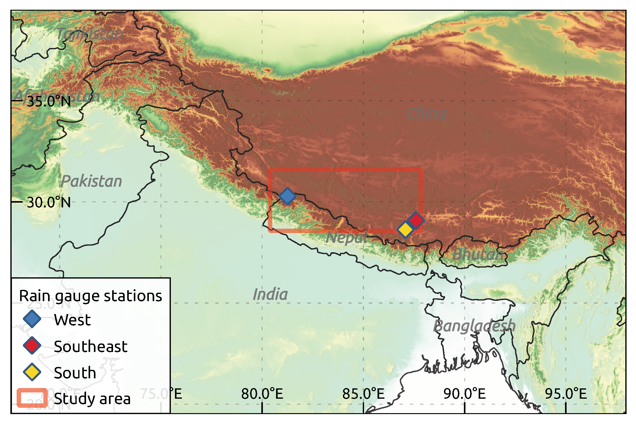
The scope of this study is to compare the global reanalysis datasets ERA5 [25], ERA5-Land and ERA-Interim [25,26], the Japanese 55-year Reanalysis (JRA-55) [27] and the Modern-Era Retrospective analysis for Research and Applications, Version 2 (MERRA-2) [28], the regional WRF-downscaled High Asia Refined analysis version 2–10 km domain (HAR v2 10 km) [29] and High Asia Refined analysis version 2–2 km domain (HAR v2 2 km) [29] gridded products, the station based precipitation dataset Global Precipitation Climatology Centre (GPCC) and the satellite derived precipitation product Precipitation REtrieval covering the TIbetan Plateau (PRETIP) [30,31]. Further information on spatial and temporal resolutions of the datasets and websites for data downloads are shown in Table 1. In a case study, we compared these datasets over a data-scarce sub-region covering each parts of the Tibetan Plateau (TiP), the Himalaya and the Himalaya foothills to the south during May to September 2017. To achieve a comprehensive intercomparison, we combined and extended different commonly used methods to inter-compare precipitation datasets and quantify differences based on terrain complexity. We finally compared gridded to rain-gauge data from the Chinese Ministry of Water Resources.
Comparable, longer-term comparisons across HMA have been carried out by e.g., Li et al., [20], who found that grid resolution plays a significant role in overall mean precipitation and local maximum precipitation, that observation-derived datasets are likely to underestimate precipitation due to their locations in the valley bottoms and that satellite products show high uncertainties, especially for solid precipitation. Similarly, Gao et al. [4] used precipitation indices to compare ERA-Interim reanalysis with WRF-downscaled products based on ERA-Interim and the community climate system model (CCSM) for the historical period and future projections over the Tibetan Plateau. They found that both ERA-Interim and CCSM greatly overestimate mean and extreme precipitation indices when compared to observation data. The dynamically downscaled products generally outperform their forcings in terms of absolute precipitation accuracy, and spatial and temporal patterns, indicating the importance of resolving small-scale processes. Similar conclusions were drawn by Huang and Gao [19], stating that ERA-Interim and final analysis data from the Global Forecasting System (GFS-FNL) datasets largely overestimate precipitation over the Tibetan Plateau (TiP). This wet bias is reduced in WRF-downscaled products. Further work by Yoon et al. [21] studied the terrestrial water budget over HMA, comparing different gridded precipitation data as boundary conditions for land surface models, including the older HAR (High Asia Refined analysis) version [32]. Mean estimates of precipitation were found to differ significantly between products, while the spatial patterns and seasonality were reasonably captured in all products. The first HAR version has also been evaluated by Pritchard et al. [33], who found that it is capable of representing precipitation in the Upper Indus Basin at multiple scales and matches ground observation data well. Furthermore, Wang and Zeng [7] used several predecessors of the current study over the TiP and found that the Global Land Data Assimilation Systems (GLADS) data has the overall best performance for precipitation when compared to station data over the 1992–2004 period. GLDAS is derived as a combination from surface observations and remote sensing. Additionally, Bai et al. [22] investigated different precipitation datasets over the Qinghai-Tibet Plateau, highlighting the importance of precipitation data in data-scarce regions and complex terrain such as the TiP. In their study satellite products, blended satellite and gauge station measurements, and climate modeling data, such as the HAR dataset, have been compared. They conclude that extreme precipitation is generally overestimated, while light precipitation (less than 1 mm day−1) was mostly underestimated by most products.
In our study, we complement those earlier studies by including the new and even higher spatially resolved HAR v2 10 km and HAR v2 2 km datasets, and by applying additional ways of comparing different gridded precipitation datasets. We emphasize that differences between datasets must be discussed based on season, precipitation type and spatial context. With a set of selected analysis methods, our aim was to address the following key research questions: (1) How similar are the various gridded precipitation datasets? (2) What is the effect of terrain complexity on variations in precipitation between products?

2. Data and Methods

In order to address the proposed question, we compiled a set of methods to compare the datasets. Similarities and differences are mostly related to grid-cell based values and how the various products represent precipitation at the same location and the same time or period. In this section, we present the study region, the datasets used for the intercomparison and the methods applied to address similarities and differences.

2.1. Study Area and Period

The study area encompasses parts of the TiP, the Himalayas and the Himalaya foothills (Figure 1). It stretches from 81° E to 88° E and from 28° N to 32° N (about 230,000 km2). We chose this study area to include different topographic features, and to represent the transition from the central parts of the Himalayas to the Tibetan Plateau and the Transhimalaya. From southwest to northeast, the first part represents the low-lying southern slopes of the Himalaya, followed by the extreme relief of the Himalayas, and the less complex TiP terrain. The study period was set from May to September 2017, which is the first year in which PRETIP precipitation can be considered. Further, the period covers a full Indian Summer Monsoon season, which exhibits the most interesting features in precipitation for any kind of research application in the study area. The 2017 monsoon season was also unobtrusive in the amount and length of the monsoon precipitation, making it a suitable study period. The choice of the study area was further motivated in the course of follow-up research by Kropáček et al. [34] dealing with glacier lake outburst floods in the Limi Valley originating from the small Halji glacier in northwestern Nepal, which is located within the boundaries of the present study area (close to the west-station in Figure 1).

2.2. Data

The datasets used in this study and their respective properties are listed in Table 1. For comparison purposes, all datasets were aggregated to daily sums. As with other precipitation datasets that do not cover either the study period or study area, we have excluded the Aphrodite dataset [35] from the analysis in this study, which is often used in precipitation comparisons in Asia.
European Centre for Medium-Range Weather Forecasts datasets. In the framework of their so-called reanalysis project the European Centre for Medium-Range Weather Forecasts (ECMWF) offers different atmospheric reanalyses. With the exception of their global coverage they differ in spatial and temporal resolution, in temporal coverage (cf. Table 1) and in the applied parameterizations. In the present study, we used the three latest products ERA-Interim, ERA5 and ERA5-Land. Please note that ERA5-Land uses the same atmospheric forcing as ERA5, interpolating the data to a higher grid resolution (see ERA5-Land documentation (https://confluence.ecmwf.int/display/CKB/ERA5-Land%3A+data+documentation#ERA5Land:datadocumentation-LandSurfaceModel)). Therefore, it was not expected to see considerable differences between ERA5 and ERA5-Land. The gridded output variables have been downloaded from the Copernicus Climate Change Service (C3S) Climate Date Store.
High Asia Refined analysis version 2. The High Asia Refined analysis version 2 (HAR v2) is an atmospheric dataset generated by dynamical downscaling of ERA5 reanalysis data. The regional climate model used for this purpose is the Weather Research and Forecasting model version 4.1 (WRF V4.1, [38]). In contrast to traditional regional climate simulations, WRF is re-initialized daily and integrated over 36 h with the first 12 h discarded as spin-up time. The HAR v2 provides meteorological fields at 10 km grid spacing and hourly temporal resolution. The 10 km domain covers the whole TiP and the surrounding mountains. The HAR v2 is described in detail by Wang et al. [29]. The dataset currently covers the period from 2004 to 2018 and will be both extended back to 1979 and updated continuously into the future. To investigate the influence of horizontal grid spacing on precipitation simulation, ERA5 has also been downscaled to 2 km grid spacing using WRF V4.1 for the study area from April 2017 to October 2017 (hereinafter HAR v2 2 km). The model setup for HAR v2 2 km was the same as HAR v2 10 km, except that no cumulus parameterization scheme was used for HAR v2 2 km and cumulus convection was thus explicitly resolved.
Precipitation REtrieval covering the TIbetan Plateau. PRETIP is a new satellite-based precipitation retrieval dataset for the TiP and originates from a feasibility study, which aimed at the combination of the brightness temperatures from the geostationary satellites Insat-3D and Elektro-L2 for precipitation retrieval [39,40]. PRETIP was trained using a random forest approach. The reference for the model training is GPM (Global Precipitation Measurement Mission) IMERG (Integrated Multi-satellite Retrievals for GPM) from which only the rain gauge calibrated microwave precipitation data are used [41]. Gauge calibrated microwave precipitation is the most reliable precipitation estimate from space thus far [18,42,43]. The temporal coverage is restricted to May–September 2017 due to the limited availability of Elektro-L2. PRETIP has the same temporal resolution as IMERG, which is 30 min, and is available in both 11 and 4 km resolutions. This increase in resolution from 11 to 4 km constitutes the advantage of PRETIP over IMERG. The spatial coverage is confined by the Tibetan Plateau and areas above 2500 m a.s.l., which does only partly cover the study area (c.f. Figure 5). Further, PRETIP is limited by the availability of microwave data, which are not available for every single 30-min timestep. Scenes for which no microwave based precipitation but satellite data (Insat-3D, Elektro-L2) are available were modeled using a daily model, which was built from the microwave based precipitation available on that day. However, due to the lack of availability of Insat-3D and Elektro-L2 at some time slots, some data gaps exist. Therefore, the daily product only contains the available timesteps. The number of available scenes per day is illustrated in Figure A1 in the Appendix A. For further details about PRETIP please refer to Kolbe et al. [30,31].
Japanese 55-year Reanalysis. JRA-55 is the second reanalysis project carried out by The Japan Meteorological Agency [27]. Observations used in JRA-55 consist of those used in ERA-40 [44] and an additional array of observations listed in the former paper. The product utilizes a four dimensional variance analysis (4D-VAR) for data assimilation. The spatial resolution is 0.56° × 0.56° and it covers the period from 1958 to near real-time. We obtained the dataset through The Data Support Section facilities at the National Center of Atmospheric Research, and for purposes of the paper, accumulated 6-hourly precipitation values to daily sums.
Modern-Era Retrospective analysis for Research and Applications, Version 2. MERRA-2 is the second version of the Modern-Era Retrospective analysis for Research and Applications produced by NASA’s Global Modeling and Assimilation Office. It replaces its predecessor, MERRA, by including additional observations and updates to the Goddard Earth Observing System model and analysis scheme. It has been available in 1-hourly temporal resolution and 0.5° × 0.625° spatial resolution in near real-time since 1980.
Global Precipitation Climatology Centre. The GPCC First Guess Daily Product is a global gridded daily precipitation estimate based on station data. The measurements undergo automatic quality control, and are interpolated between grid cells using an ordinary block kriging [37]. The spatial resolution of the grid is 1° latitude by 1° longitude and the dataset is available from January 2009 until near real-time. Within our study area, a total of three gauge stations are used to derive daily precipitation.
Ground observations. For a ground validation of the precipitation products we resorted to the collection of precipitation data provided by the Chinese Ministry of Water Resources and collected by the hydrometerological service of Tibet. The amount of precipitation was measured by tipping bucket rain gauges installed according to World Meteorological Organization standards over the period 2007–2015. The network, albeit sparse given the size of the area, provides the only set of ground observations available to assess the gridded precipitation datasets. The stations of network used in this study are shown in Figure 1.

2.3. Methods

2.3.1. Correlation Coefficient

To compare the different precipitation products, we used the non-parametric Spearman’s rank correlation coefficient, R, which describes how similar the spatial pattern of precipitation is within the compared grids on a daily or multi-daily basis. Due to the different spatial resolutions, for each pair of products, we aggregated the higher resolution product to match the grid resolution of the lower resolved product within each comparison. Similarities between various generations from the same source (ERA products) and different spatial resolutions of the same product (HAR v2 products) can help to assess variations resulting from diverse methodologies and parameterizations in the generations of these datasets. We used different temporal aggregation intervals to assess whether the timing of precipitation events is different within the products and whether multi-day-sums increase their similarities. Correlations were only derived for grid cells with valid values in both datasets.

2.3.2. Comparison to Station Data

To obtain an approximation of ground truth precipitation, we utilized three rain-gauge stations within our study area that provide daily precipitation sums. We compared their cumulative sums over the study period to the cumulative sum of the respective grid cell in the precipitation products. We extracted the elevation of each station from the Advanced Land Observing Satellite (ALOS) Digital elevation model (DEM), provided by ALOS World 3D—30 m (AW3D30) of the Japanese Aerospace Exploration Agency (https://www.eorc.jaxa.jp/ALOS/en/aw3d30/index.htm). The stations’ elevations were then compared to the modeled elevation of the grid cell for the reanalysis and WRF-downscaled products, and to the mean elevation of the grid cell for PRETIP and GPCC (derived from ALOS, Table 2). These comparisons provide insights into the possible reasons for differences between ground-based weather station observations and gridded reanalysis or satellite data, because the generation of several products relies on the topography, and thus the resolution of the underlying digital elevation model.

2.3.3. Climdex

Climate indices are usually used to quantify how climate has changed over long periods, how it differs in space or to identify and track climate extremes (e.g., [45]). In this study, we used a set of climdex indices to compare the different precipitation datasets similarly to Gao et al. [4]. The indices used in this study are R1, R10, R20, Rx1, Rx5 and PTOT. They were calculated for every grid cell and summarized for the different products. An overview over the different indices and their definitions is given in Table 3.

2.3.4. Terrain Complexity

There are various options to geometrically and statistically define terrain complexity [46]. In this study, we assessed the influence of terrain complexity on the differences between the precipitation datasets on the basis of the ALOS DEM, as illustrated in Figure 2. Two levels of complexity are defined by the standard deviation (SD) of elevation from the high resolution ALOS-grid cells within single grid cells according to the product with the lowest resolution (GPCC). Complexity is defined as low or high based on the percentiles of SD of grid cells. For high complexity, we set a threshold at the 75% percentile (Q3) of SD among all grid cells. This means that 25% of the grid-cells above this threshold are classified as “high complexity.” The remaining 75% of the grid-cells represent “low complexity.” For each product, we calculated the mean difference between the products with regard to terrain complexity in order to derive its potentially varying influence on rainfall calculation. In order to compare products with different spatial resolutions, we resampled all products to the coarsest common denominator grid (GPCC, 111 km, 24 grid cells).

3. Results

3.1. Statistical Analysis

In this section, we describe and visualize the datasets used for comparison and the results of the statistical analysis.
To illustrate how the different precipitation products compare within the study region and period, we provide the cumulative sum of precipitation from May to September 2017 (Figure 3), the sum of precipitation for each month within the study period (Figure 4), and a spatial plot with per-pixel sums over the study period (Figure 5).
Overall, the per-pixel sum (cf. Figure 3) is between 600 and 800 mm for all ECMWF products, the WRF-downscaled HAR products and JRA-55. MERRA-2 and GPCC only show 400 to 500 mm of precipitation, which results in a difference up to 100% between the datasets. Despite the missing lower-lying areas (<2500 m a.s.l.) and the fact that the daily values are built only from available satellite scenes, PRETIP amounted to 525 mm for the period between May and September 2017, which falls within the range of the other datasets.
Monthly sums (Figure 4) show that all products have their maximum precipitation in July and August, while September has the lowest values. The relative variability between datasets is greatest in the pre-monsoon season (May), while the agreement is best between most datasets in July to August (except for MERRA-2, PRETIP and GPCC). Other than for PRETIP, for which no valid values in the southwestern corner of the study area exist due to the elevation below 2500 m, the other datasets generally show highest precipitation sums in the southwest along the foothill of the Himalayas, and lowest values occur along the transition from the Himalayas to the TiP. The Himalaya range generally shows the highest spatial heterogeneity as long as the spatial resolution is sufficient to depict these small-scale changes (Figure 5). In general, it can be seen that only the HAR v2 datasets and in parts the ERA5 products are able to resolve orographic precipitation, while the resolution of the other products only gives grid values based on averages in the area. Surprisingly, the satellite product PRETIP, which has the second highest grid resolution (4 km) is not able to capture small-scale patterns of topographically-induced precipitation.
The correlation on a daily basis for each combination of datasets is given in Table 4. The highest correlation was achieved between ERA5 and ERA5-Land, with R = 1, while lowest correlation was found between the reanalysis product MERRA-2 and the satellite dataset PRETIP (R = 0.33). In general, the correlation between the ERA products and the ERA-derived products (HAR v2 10 km and HAR v2 2 km) is quite high (R > 0.66), suggesting that their precipitation values depicting the most probable range (cumulative values of 600–800 mm, c.f. Figure 3). The fact that they are not identical, however, shows that there are also considerable differences between the datasets, which is most likely the effect of different representations of precipitation processes at different scales and the different representations of cumulus convection in the models.
Temporally aggregating precipitation over a 5-day window generally increases the correlation (Table 5). The highest correlation can still be found between ERA5 and ERA5-Land (R = 1), but the lowest correlation can now be found between the observation-based product GPCC and the satellite product PRETIP (R = 0.56). In general, PRETIP shows the overall smallest correlation to all other products. With a mean of 0.63 and generally similar values regarding the comparison to the other datasets, PRETIP appears to have the largest differences in overall grid-based precipitation. Further aggregation of precipitation over ten days and entire months did not significantly increase correlations, indicating that most differences in the timing of precipitation between products are covered within a 5-day period (see Table A1 and Table A2).

3.2. Comparison with Rain Gauge Data

Daily values from rain gauge stations and grid values from the daily precipitation products are cumulatively summed up over the study period as illustrated in Figure 6. In general, the station data shows significantly lower values than most of the gridded products. Exceptions can be seen at the south station, where both HAR products show lower cumulative sums than the observations at the station. At the southeast station, the observed values are almost identical to the grid values of MERRA-2 and GPCC, while both HAR products only show slightly more precipitation by the end of the study period. A similar trend can be seen in the south station, where the before mentioned products represent the observations best. The other products generally show more precipitation than what is observed at these stations, up to four times as much. The west station is located in a generally dry valley, which receives, on average, less than 200 mm of annual precipitation [47]. This can be seen by the total cumulative precipitation observed at the station of only 64.6 mm. The closest gridded values are again MERRA-2, GPCC and HAR v2 2 km with about 250 mm. While both HAR products show very similar values at the south and southeast station, they are fairly different at the west station with the 10 km resolution product showing almost twice as much precipitation as the 2 km product. ERA-Interim, on the other hand, greatly overestimates precipitation in this grid-cell by 24 times as much precipitation as observed by the station. In general, the timing of precipitation is better represented between station and gridded product than the actual amount. Most products agree on the majority of precipitation falling between June and August and little precipitation from August until the end of the study period. However, the absolute differences between observed and gridded precipitation are, in parts, substantial.

3.3. Terrain Complexity

The magnitude of difference in precipitation with respect to terrain complexity is given in Figure 7. Overall, it can be seen that the difference in precipitation is consistently higher in complex terrain (red dots, SD > Q3), than in less complex terrain (blue squares, SD ≤ Q3). The biggest difference in precipitation can be seen between PRETIP and HAR v2 10 km with 3.9 mm d−1 followed by PRETIP and MERRA-2 with 3.7 mm d−1, and PRETIP and ERA-Interim with 3.6 mm d−1. Visually, the differences based on terrain complexity can be distributed in different groups: (i) overall low differences and small variation between high and low complexity pixels (e.g., HAR v2 10 km and ERA5-Land), (ii) overall higher differences, but small variation between high and low complexity pixels (e.g., GPCC and JRA-55) and (iii) differences spread out greatly between low and high complexity (e.g., PRETIP and HAR v2 10 km). The lowest mean difference can be seen between ERA5 and ERA5-Land with only 0.2 mm d−1, which further affirms that the forcing in ERA5-Land is the same as in ERA5 and that interpolation is done linearly. The second-lowest mean difference can be seen between HAR v2 2 km and HAR v2 10 km with 0.9 mm d−1. The overall mean difference between products (yellow diamond) is between 1 and 2.5 mm d−1, with the highest value between GPCC and ERA-Interim, the two products with the coarsest grid resolutions. Overall, for low complexity terrain, most precipitation differences are between 0 and 2 mm d−1 while high complexity differences mostly range between 1.5 and 4 mm d−1.

3.4. Climdex Indices

With the climdex indices, we aim at quantifying precipitation extremes for each product and compare the spatial mean. Figure 8 shows boxplot charts for each index where every value represents a single grid cell within each product. In this representation, grid resolutions were not aggregated in order to capture the full range of grid values in each product. To be able to compare the products universally, we additionally compiled an equivalent representation of the same indices but with the same coarse grid resolutions. The resulting illustration can be found in the appendix (Figure A2a). Similar overall values were found in both versions but maximum values are considerably smaller due to the spatial aggregation. In order to allow for a more straightforward comparison of original and spatially aggregated climdex data, in Figure A2b we include the data behind Figure 8 but with the scaling as used in Figure A2a. The following presentation and discussion of the results will focus on the climdex indices based on the original spatial resolution of each precipitation product as presented in Figure 8. In general, it can be seen that the higher the spatial resolution, the larger is the data range between all grid cells (except for PRETIP).
Data points for days with more than 10 and 20 mm of precipitation (R10 and R20), show that the higher resolved products (HAR v2 10 km and HAR v2 2 km) return the overall highest values while they have much lower mean values and lower maximum values for the general wet-day count (R1). This implies that individual grid cells in higher resolved products (e.g., HAR v2 2 km) can experience more extreme precipitation events in multiple grid cells than coarser products (e.g., ERA-Interim). Higher overall median values in the extreme precipitation indices (R10 and R20) in the higher resolved products further imply the resolution of locally confined heavy precipitation events. Continuing with the extreme event indices (Rx1 and Rx5), it can be seen that the highest values can also be found within the higher resolved products, followed by a decreasing trend with decreasing grid resolution. However, it needs to be mentioned that in contrast to HAR v2 2 km, in which convective systems are explicitly resolved, HAR v2 10 km uses a cumulus parameterization scheme, which has some uncertainties and can, in rare occasions, lead to extremely high values, such as more than 500 mm in one day, which can not be found in any of the other products. The third-highest amount of precipitation in a single day (Rx1) can be found within ERA5 and ERA5-Land with about 140 mm. Over a 5-day period (Rx5), the maximum values increase to 700 and more than 800 mm in the HAR v2 10 km and HAR v2 2 km products, respectively, while ERA5 and ERA5-Land range between 200 and 300 mm.
Total precipitation in a single grid cell is highest in HAR v2 2 km with a maximum of 7865 mm in a single grid cell. It is followed by HAR v2 10 km with 5217 mm and ERA5 with 2317 mm. MERRA-2 has the lowest maximum total precipitation with only 1100 mm over the study period. Comparing the two products with similar spatial resolution, ERA5-Land and HAR v2 10 km difference between linear interpolation and WRF-downscaling become obvious. While the grid-cell with the maximum PTOT in ERA5-Land amounts to 2400 mm, the maximum in HAR v2 2 km amounts to 7865 mm, which is more than three times as much compared to ERA5-Land within the 5 month-period.
Figure A2 reveals that the outstanding maximum values of the two HAR v2 datasets in Rx5 and PTOT are mainly a consequence of higher spatial resolution. As soon as spatial resolution is equalized by spatial aggregation, the maximum values are very much different, and the two HAR datasets do not show extra-ordinary values. In fact, in the spatially aggregated version (Figure A2a) the GPCC dataset shows the highest maximum value of Rx5, indicating that interpolation of station measurements to larger areas may negatively impact hydrological modeling.
Notably, despite its second-highest grid resolution, the satellite product PRETIP shows the smallest variation regarding precipitation rates within grid cells and few outliers in all indices, which relate to the overall more homogeneous distribution of precipitation throughout the study area in this product (c.f. Figure 5).

4. Discussion

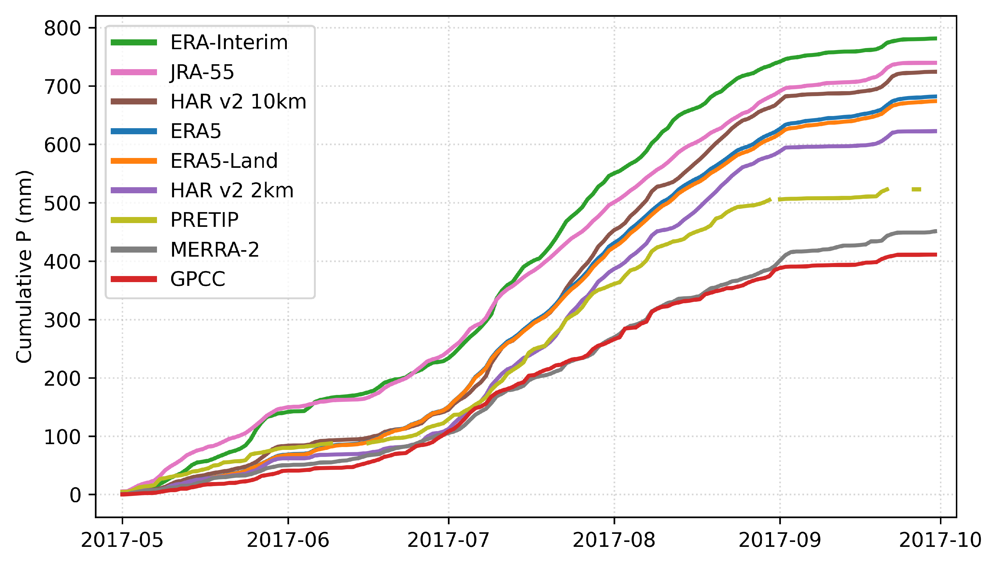
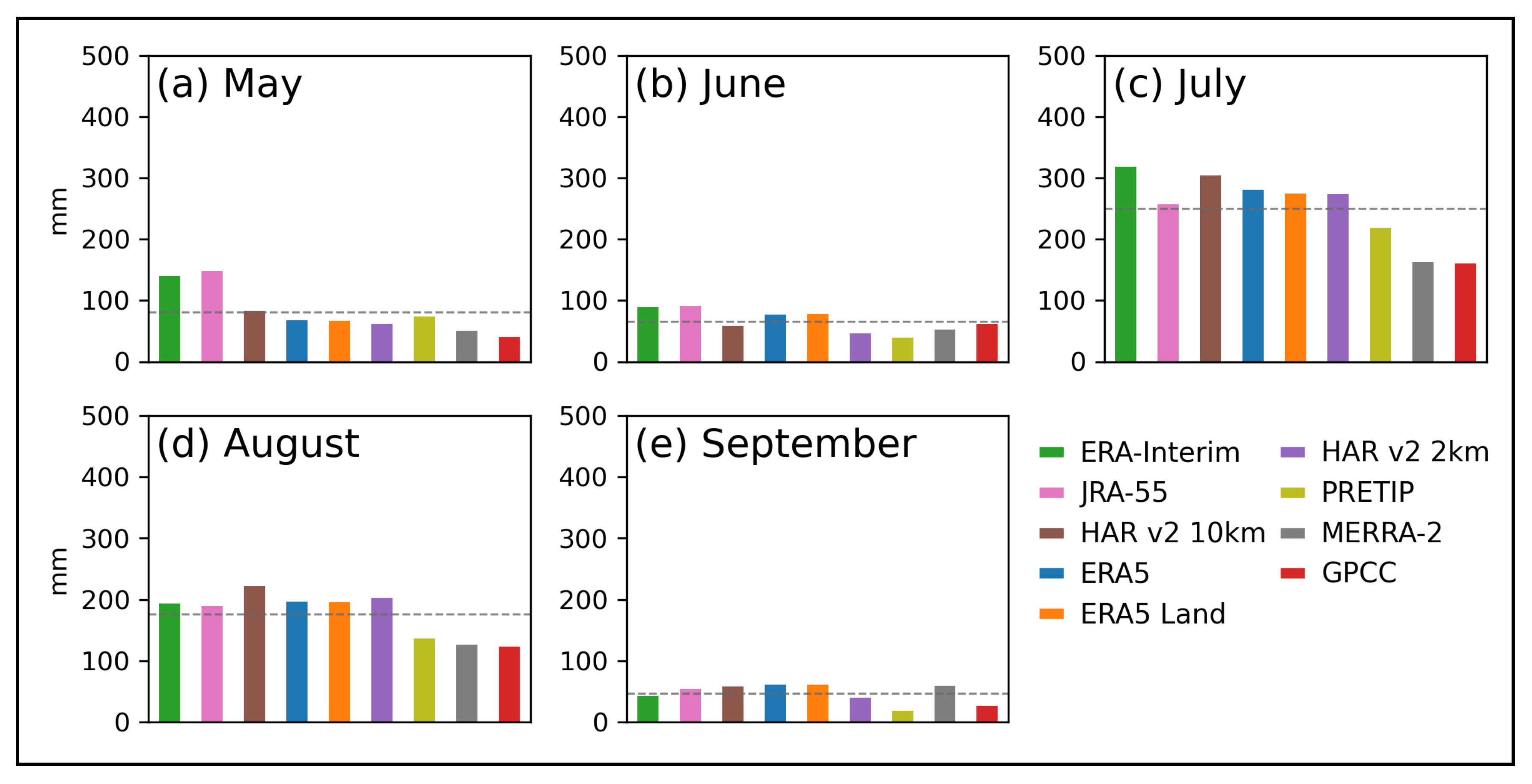
Despite the short period of analysis presented, it is possible to discover substantial similarities and differences between the different gridded precipitation products over the study area. As observed in Figure 3, the study area is influenced by the Indian Summer Monsoon which becomes visible in the increase of precipitation during July and August and its withdrawal starting in September. Most products show a good agreement within the monsoon season, except for PRETIP, GPCC and MERRA-2. In addition, the area is also affected by the westerlies, which becomes visible in the pre-monsoon season (May). The inconsistency between JRA-55 and ERA-Interim and all other datasets might originate from different parameterizations for westerly-driven mostly solid precipitation. Combined, it appears that ERA5, ERA5-Land, HAR v2 10 km, HAR v2 2 km and for the most part PRETIP consistently match both the pre-monsoon and monsoon precipitation, while the remaining datasets have limitations in either one of those two periods.
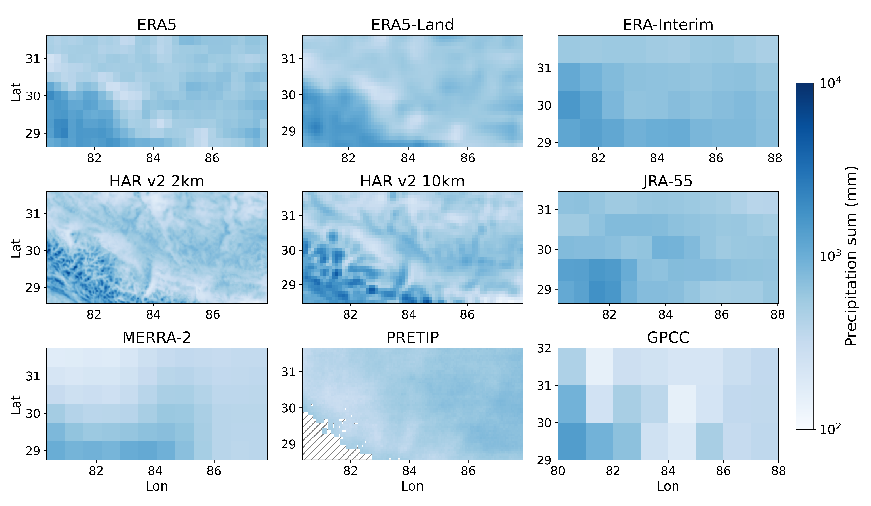
Based on the correlation between datasets, it became obvious that some are more similar than others. ERA5-Land and ERA5 are essentially identical when aggregating ERA5-Land to ERA5 resolution. This is to be expected, as ERA5 is using ERA5 atmospheric forcing to derive land-surface parameters. Hence, it should be noted that ERA5-Land does not add any value regarding orographically-induced precipitation over ERA5 when using atmospheric data. While all the ERA products and the ERA5-derived HAR products generally are very similar, the satellite product PRETIP exhibits the lowest correlations, even after aggregating precipitation over multiple days. Considering the spatial patterns of PRETIP precipitation, it is no surprise that the correlations are low. While the other products show a spatially decreasing trend in precipitation from southwest to northeast with a highly variable region in the Himalaya mountain range, PRETIP exhibits a much more homogeneous distribution throughout the study area. It even shows lower values for the Himalaya mountain range than the area covering the TiP. This is a result of the averaging character of the random forest algorithm which is smoothing for more extreme (low and high) precipitation and tends toward average precipitation rates. In future developments, the training should be either separated for convective and stratiform precipitation, or another machine learning algorithm that better captures meteorological extremes should be developed [48,49]. On the other hand, the similarities between the ERA products, the HAR products and to some extent JRA-55 lead to the conclusion that these products display the most likely range of precipitation in this study. The differences between those modeled datasets can be attributed to differences in model dynamics. This is in line with Zhang and Li [50], who found that differences in moisture advection parameterizations greatly change precipitation patterns on steep slopes. It is not possible to ultimately say how well these products match the “true” precipitation. However, the few observations that are available suggest that the above mentioned products are the ones with precipitation amounts being the closest to actual precipitation amounts.
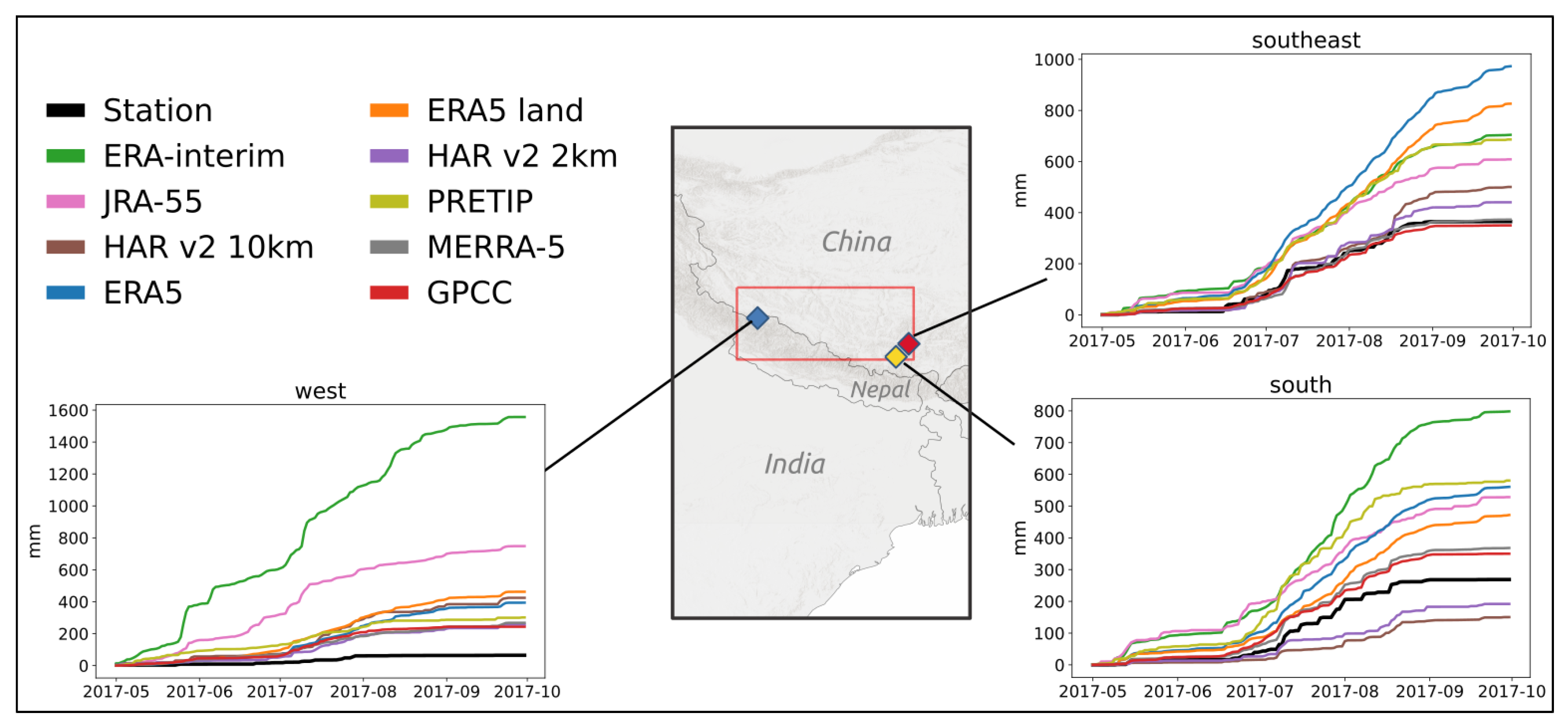
The comparison with rain gauge station data revealed that both HAR v2 datasets have the best matches with the ground observations. For the south and southeast stations, they also show very similar values, though they are more different at the west station. Here, the gauge station is located in a very localized, dry area, making local processes even more important. While these processes seem to be better represented in HAR v2 2 km, the 10 km grid seems to catch precipitation that might be outside the confined dry area. Considering ERA-Interim in this comparison, it becomes obvious that the extremely coarse grid resolution must be covering areas with higher precipitation outside the dry valley the station is located in. The elevation comparison between modeled elevation of ERA-Interim and the DEM-extracted elevation of the rain gauge station (Table 2) shows that the station is located higher (4134 m a.s.l) than the modeled elevation of the ERA-Interim grid cell (3573 m a.s.l.). However, even though it is to be expected that stations located in low-lying areas would exhibit less precipitation than higher-lying areas, ERA-Interim shows much higher values than the gauge station, which emphasizes the limitations of trying to explain precipitation discrepancies by solely considering altitude as the determining factor. The good match between GPCC and the ground observations can be attributed to the fact that GPCC synthesizes station-based data and interpolates between them. Hence, it is to be expected that GPCC scores high correlations with surface observations in grid cells with observations, making it useful for individual grid-cells. However, the heavily interpolated values in between distant station data are subject to extreme uncertainties as no topograhical and regional features can be captured. Generally, rain gauge stations are often located in valley bottoms and easily accessible areas. Precipitation at the adjacent mountain peak or on its slopes might be higher, which can be represented by the modeled data, but not by rain-gauge station observations.
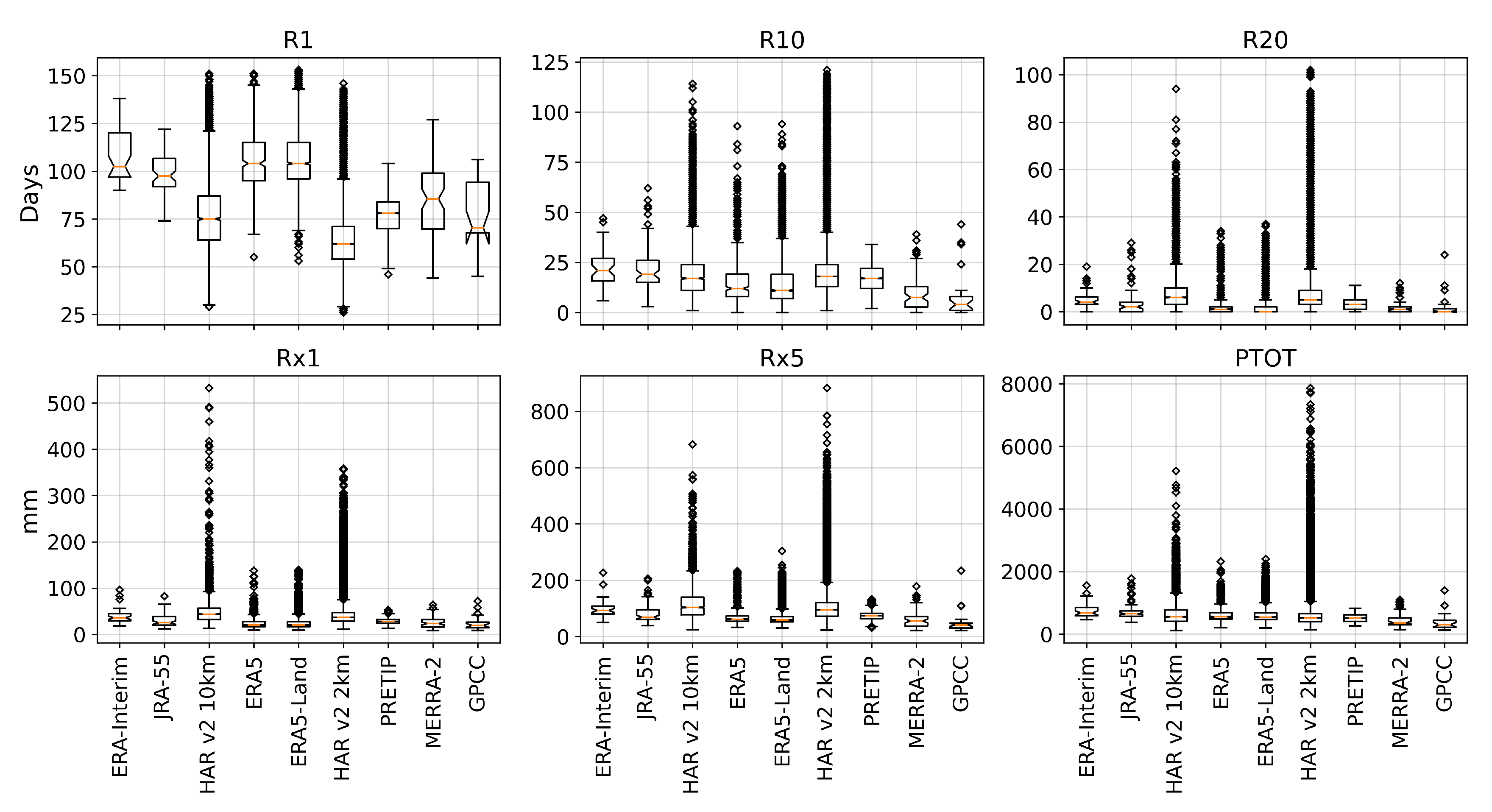
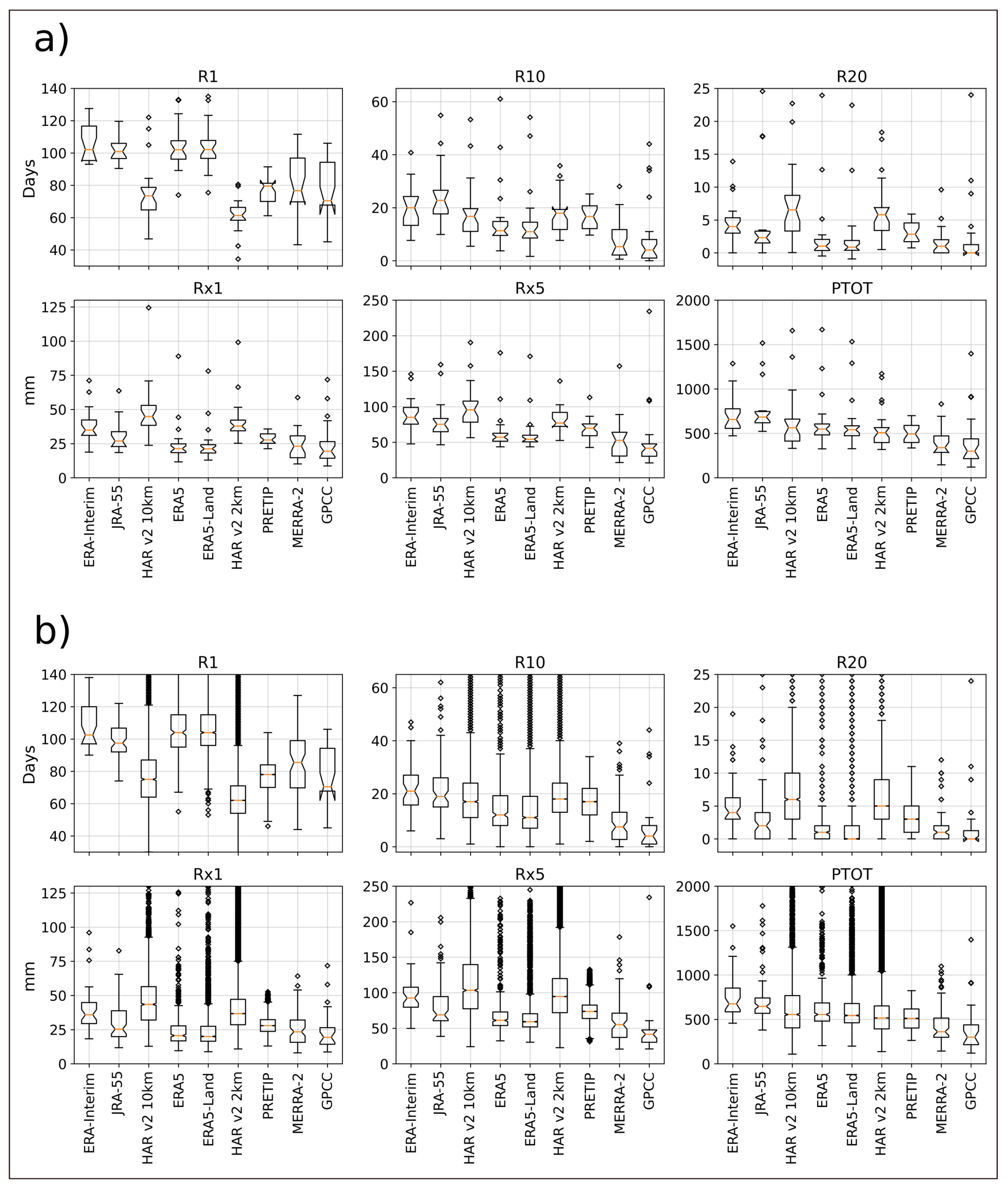
With the six climate indices (climdex) we found that the products with the highest grid resolution exhibited the highest number of days with heavy precipitation (R10 and R20) and the largest amount of precipitation in a single day and five consecutive days (Rx1 and Rx5). On the other hand, the mean values of the wet-day count (R1) were much smaller, which is an improvement compared to ERA-Interim precipitation in particular. According to Gao et al. [4], ERA-Interim tends to overestimate precipitation on average, especially in the frequency of precipitation events. With the mean values of R1 in both HAR datasets in our case study being much lower than those in ERA-Interim, they seem to better represent the distribution of precipitation. The same feature, albeit lower in magnitude, can be observed between ERA-Interim and ERA5, indicating an improvement of precipitation representation between the two generations of ECMWF-reanalysis products in this specific case study. Overall, extreme precipitation events can occur in multiple grid cells within the higher-resolved HAR datasets. However, the cumulus parameterization in HAR v2 10 km seems to produce extremely high values of more than 500 mm in a single day, which does not happen in the 2 km grid version of the product. This finding is in accordance with Ou et al. [51], in which high-resolution WRF experiments with and without cumulus convection scheme were conducted at a gray-zone grid spacing of 9 km. They found that the experiment without a cumulus scheme generally outperforms the experiments with cumulus schemes in terms of the mean total precipitation, and the diurnal cycles of precipitation amount and frequency. The total precipitation (PTOT) for all products shows that the maximum amount of a single grid cell can vary between less than 2000 mm up to almost 8000 mm. It became obvious that this cumulative difference in precipitation over only five months will strongly impact on the results of research applications if either one or the other product is chosen for the specific location.
Overall, our findings in terms of spatial resolution are in line with other studies, suggesting that higher grid resolution is needed to accurately represent terrain-induced precipitation patterns [20]. In this study, only the HAR datasets and partly the ERA5 datasets were able to represent large orographic complexity. However, an increase in spatial resolution does not always yield higher accuracy in complex terrain, as can be seen within the PRETIP product, which is much more homogeneous than some of the lower resolved products. On the other hand, the coarsest product GPCC might perform much better in areas where individual grid cells contain measurements, while the interpolated cells in between are subject to high uncertainties. Further, GPCC has a high probability of underestimating precipitation due to the locations of ground observation stations being in valleys rather than on slopes or mountain summit areas.
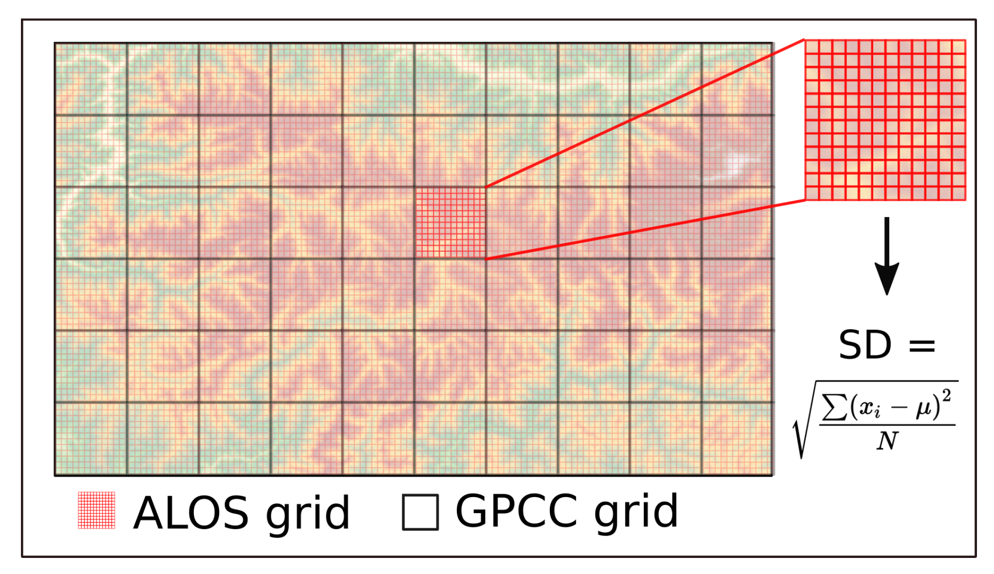
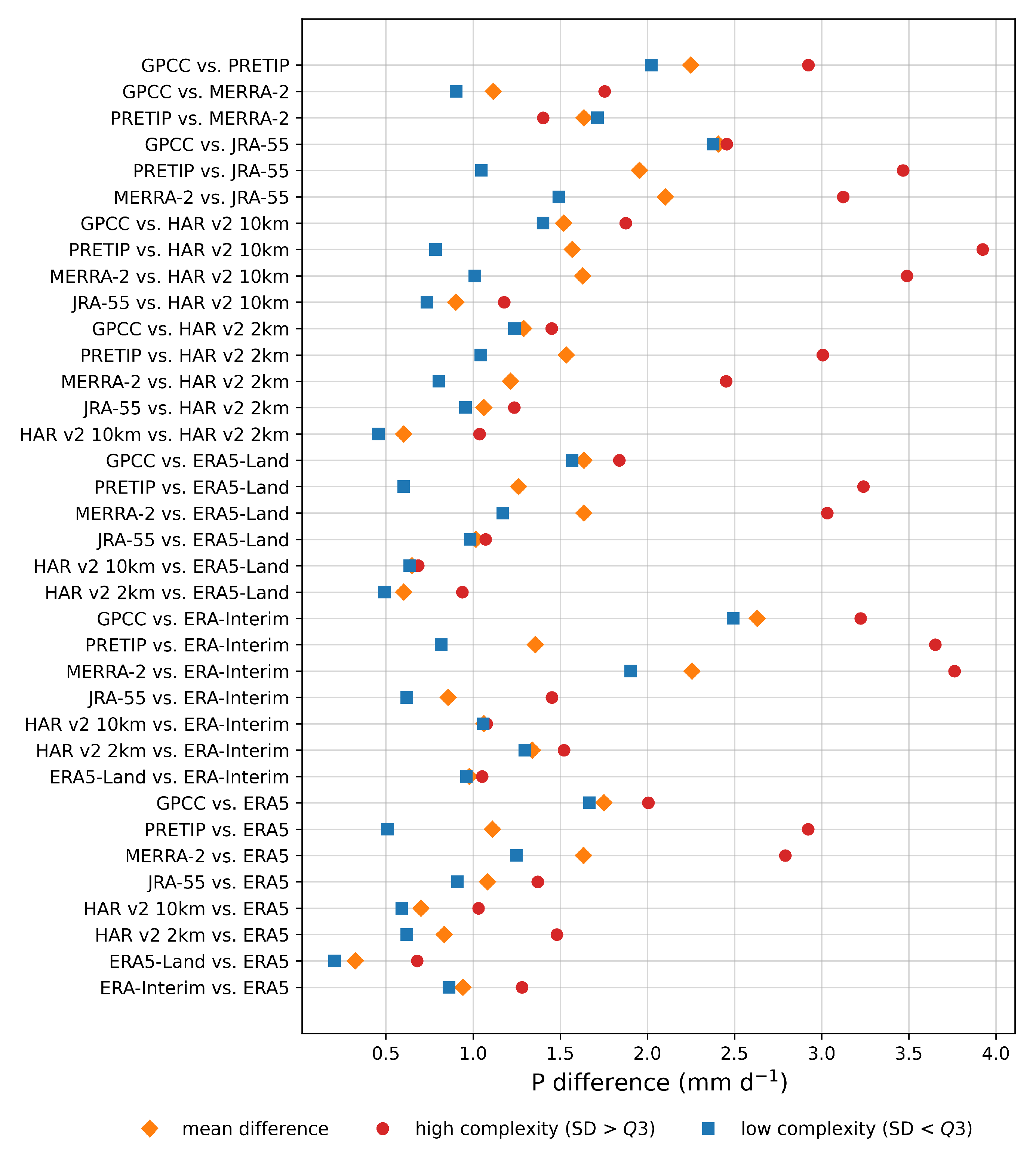
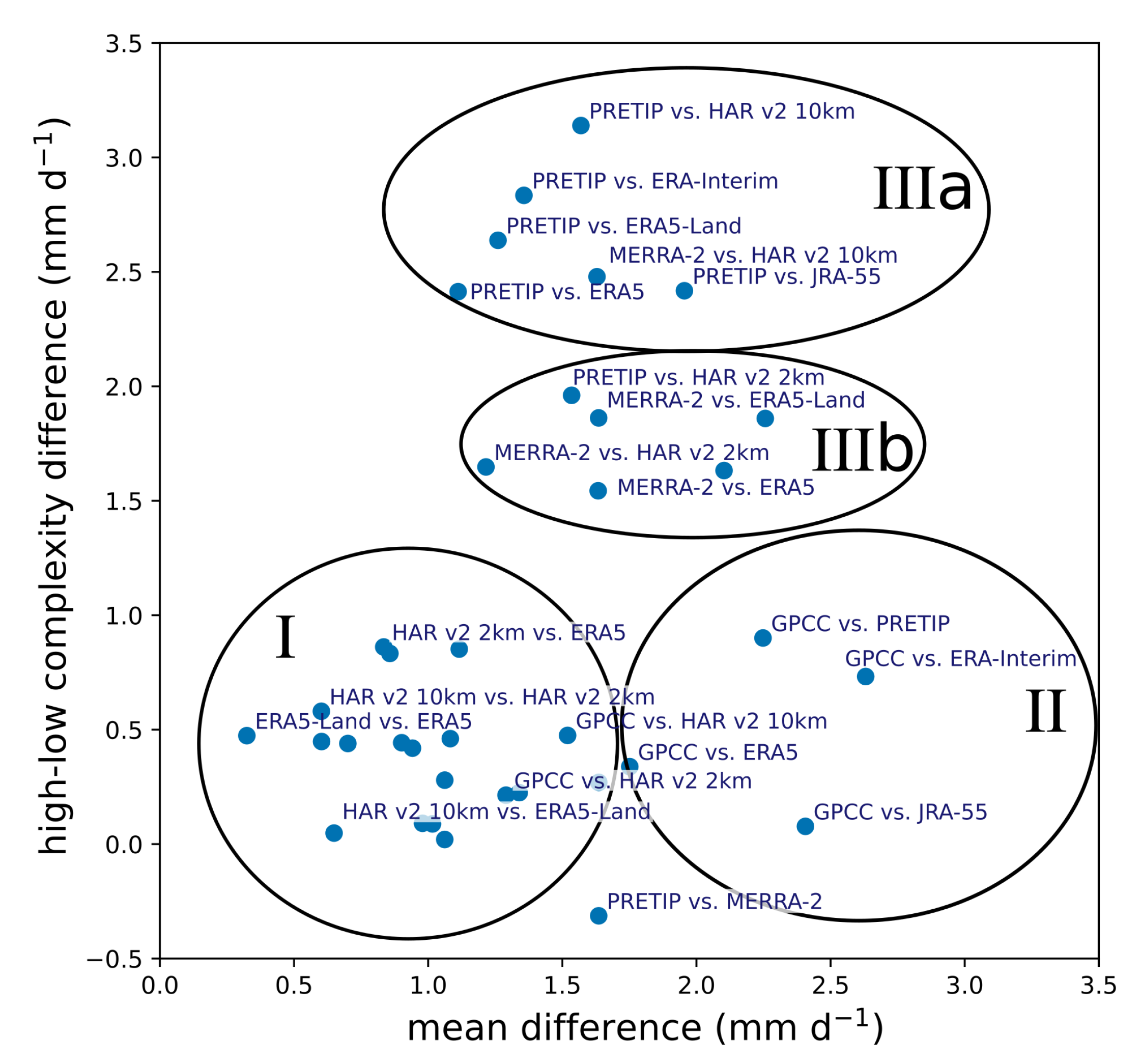
The role of terrain complexity was assessed with the help of a digital elevation model. We found that all datasets displayed higher differences in precipitation when the terrain complexity (ALOS standard deviation) was larger than Q3, except for one pair (PRETIP and MERRA-2). Based on the grouping of the pairs depending on their relationship between mean difference and precipitation, for the difference between high and low complexity terrain four main clusters can be derived (Figure 9). While cluster I includes most of the similar datasets, such as ERA and HAR datasets due to their overall similarity, cluster II comprises mostly comparisons with the coarsely resolved GPCC product. The greater overall mean difference between GPCC and the other products is most likely a result of the heavily interpolated values for grid cells without measurements. However, terrain complexity does not seem to have a significant additional impact on the differences. Cluster IIIa and IIIb are mostly dominated by comparisons with PRETIP and MERRA-2. While the differences with PRETIP are attributable to the averaging nature of the random forest approach and the resulting smoothing in complex terrain, the comparisons with MERRA-2 canot be interpreted in a straight forward way. All comparisons with MERRA-2, except for the comparison between PRETIP and MERRA-2, are grouped within cluster III, which leads to the conclusion that precipitation in terrain with high complexity within MERRA-2 seems to be weaker compared to most other products. The inverse behavior of the pair PRETIP and MERRA-2 in terms of precipitation in complex terrain vs. less complex terrain is probably attributable to the fact that this pair has the lowest overall correlation for daily values and hence has the largest differences in all grid cells, independently of topography.

5. Conclusions

This study presents the intercomparison of nine differently generated gridded precipitation products from a study area in HMA from May to September 2017. Precipitation as boundary condition for any research application can greatly influence the outcome and respective interpretation. In order to be able to understand and predict the future behavior of a system, it is necessary to apply tools, such as modeling, which require a certain spatial and temporal coverage of their input data. This is particularly challenging for remote regions with complex terrain, such as in HMA. Making an informed decision about the boundary conditions used for the respective applications is key to achieving reliable predictions and can be a difficult endeavor. In this study, we highlighted the similarities and differences of spatially and temporally continuous gridded precipitation data from various sources over one full monsoon period that can be used as boundary conditions for longer-term applications, such as climate-change assessments, runoff-calculations, glacier mass balance modeling and hydropower-applications, among others. While a product with coarse grid resolution such as ERA-Interim might be able to reproduce seasonal patterns and long-term climate trends [4], glacier modeling applications might require much higher grid resolution as for example in HAR v2 2 km, which resolves processes related to local topography much better than products based on coarser grids. However, the HAR v2 2 km product has high computational demands due to its high resolution dynamical downscaling. It is only available for distinctive study regions and periods where it is of high value to analyze the effects of grid resolution and topography. The HAR v2 10 km, on the other hand, shows very good matches with observational data and is available for a longer periods and the entire HMA. It shows slight limitations compared to the 2 km version originating from the cumulus parameterization, which can overestimate precipitation falling in a single day. Nonetheless, HAR v2 10 km is the only product (together with HAR v2 2 km) that is able to resolve topographic precipitation features (c.f. Figure 5). Similarly, gauge station data might not be representative of the wider areas due to their typical locations in areas of low-complexity terrain. Hence, products derived from station data such as GPCC might underestimate areal precipitation, especially if there are only one or two stations within a grid cell, as is usually the case in HMA. Higher grid resolution, as in PRETIP, on the other hand, might also not improve precipitation estimates, as this satellite-based product is limited to the averaging within the random-forest methodology. We therefore suggest to not only rely on a single dataset in any application but to elaborate on the potential influences of different datasets in comparison. We suggest selecting a precipitation dataset based on one’s application and requirements. For example, if data are needed for multi-decadal hydro-meteorological or hydro-climatological research applications, ERA5 is currently the best choice. When HAR v2 10 km becomes available for longer periods it will replace ERA5 in this position. If precipitation in complex terrain at high spatial resolution is to be investigated, HAR v2 2 km would be the optimally applicable dataset, which might still require bias correction for local applications. HAR v2 10 km and ERA5 might be employed over larger study areas or extended study periods. Similarly, glacio-hydrological studies, which usually expand over small areas, require high spatial resolution to accurately represent the prevailing accumulation patterns of the area. For studies focusing on the broader precipitation patterns under consideration of terrain complexity, most ERA products, the HAR products and JRA-55 have shown to be very similar. PRETIP offers a great opportunity for near-real time applications, such as flood forecasting, as the satellite data can be available within hours after the passage of the satellite, whereas reanalysis products are only available after several weeks.
Overall, in this study we elaborate and conclude on the following:
(1) How similar are the different gridded precipitation datasets? Depending on the origins and generation of the datasets, some datasets are very similar (e.g., HAR v2 2 km and HAR v2 10 km; ERA5 and ERA5-Land), while other datasets show larger discrepancies (e.g., Merra and GPCC). Despite some data gaps, the satellite product (PRETIP) falls within the range of cumulative precipitation and shows similar trends to other products. When comparing the grid values to station data, we conclude that spatial resolution plays a significant role and that gauge measurements likely exhibit a dry bias due to their locations on valley floors or other areas of low terrain complexity. However, most products represent the timing and patterns of precipitation events well.
(2) What is the effect of terrain complexity on variations in precipitation between products? Terrain complexity increases the difference of precipitation between products. In complex terrain, the difference within daily precipitation can be up to 4 mm d−1, whereas it is generally below 2 mm d−1 in more homogeneous landscapes. Overall, the differences in precipitation derived from the analysis based on terrain complexity enables one to draw conclusions on how well some products work for studies focusing on complex terrain. For instance, it is possible to use the ERA5-Land dataset rather than the HAR v2 10 km dataset, if the latter is not available. Locally, the differences can still be large, but the overall precipitation estimates over a wider area are consistent between both datasets.

Author Contributions

Conceptualization, A.H., A.A. and C.S.; methodology, A.H.; software, A.H.; validation, C.S., D.S., J.B., B.T. and P.R.; formal analysis, A.H. and A.A.; investigation, A.H., A.A.; data curation, P.R., O.B., X.W., A.A. and C.K.; interpretation of results, D.S., A.H., C.K., X.W., A.A., J.B., C.S. and P.R.; writing—original draft preparation, A.H.; writing—review and editing, A.H., A.A., C.K., X.W., J.B., D.S., C.S., P.R. and O.B.; visualization, A.H.; supervision, C.S., D.S., J.B. and B.T.; project administration, C.S., D.S. and J.B.; funding acquisition, C.S., D.S., J.B. and P.R. All authors have read and agreed to the published version of the manuscript.

Funding

This research was funded by the German Research Foundation’s (DFG) research grant “Precipitation patterns, snow and glacier response in High Asia and their variability on sub-decadal time scales.” The program consisted of the subprojects “snow cover and glacier energy and mass balance variability” (prime-SG, SCHN680/13-1), sub-projects: “Remote Sensing of precipitation” (prime-RS, BE1780/46-1 and TH1531/6-1), and “prime-HYD—High Mountain Asian HYDrological variability” (prime-HYD, RE3834/4-1). We also acknowledge support from the German Federal Ministry of Education and Research (BMBF) within the project “Climatic and Tectonic Natural Hazards in Central Asia” (CaTeNA, FKZ 03G0878G).

Acknowledgments

We greatly thank the Chinese Ministry of Water Resources and Zhiyu Liu for sharing the Chinese rain-gauge observation data for the non-profit research study within our project. We would also like to thank the three anonymous reviewers and the editors, who substantially helped to improve the study. Further, we acknowledge support by the German Research Foundation (DFG) and the Open Access Publication Fund of Humboldt-Universität zu Berlin.

Conflicts of Interest

The authors declare no conflict of interest. The funders had no role in the design of the study, in the collection, analyses or interpretation of data, in the writing of the manuscript, or in the decision to publish the results.

Abbreviations

The following abbreviations are used in this manuscript:
List of Acronyms
 
ALOSAdvanced Land Observing Satellite
DEMDigital elevation model
ECMWFEuropean Centre for Medium-Range Weather Forecasts
ERA5ERA5
ERA5-LandERA5-Land
ERA-InterimERA-Interim
GPCCGlobal Precipitation Climatology Centre
HAR v2High Asia Refined analysis version 2
HAR v2 2 kmHigh Asia Refined analysis version 2–2 km domain
HAR v2 10 kmHigh Asia Refined analysis version 2–10 km domain
HMAHigh Mountain Asia
JRA-55Japanese 55-year Reanalysis
MERRA-2Modern-Era Retrospective analysis for Research and Applications, Version 2
PRETIPPrecipitation REtrieval covering the TIbetan Plateau
TiPTibetan Plateau

Appendix A

Table A1. Correlation coefficient R for all datasets in mm/10 days. All correlations are statistically significant at the 99% confidence interval.
DatasetERA5ERA-InterimERA5-LandHAR v2 2 kmHAR v2 10 kmJRA55MERRA2PRETIP
ERA-Interim0.84
ERA5-Land1.000.84
HAR v2 2 km0.880.830.85
HAR v2 10 km0.860.840.860.89
JRA550.720.800.740.750.73
MERRA20.760.730.780.740.750.67
PRETIP0.720.740.720.710.710.720.64
GPCC0.800.730.810.750.750.690.760.58
Table A2. Correlation coefficient R for all datasets in mm/month. All correlations are statistically significant at the 99% confidence interval.
DatasetERA5ERA-InterimERA5-LandHAR v2 2 kmHAR v2 10 kmJRA55MERRA2PRETIP
ERA-Interim0.83
ERA5-Land1.000.83
HAR v2 2 km0.890.860.88
HAR v2 10 km0.870.870.870.92
JRA550.710.860.730.780.76
MERRA20.680.710.690.680.690.64
PRETIP0.710.750.740.760.720.660.51
GPCC0.740.730.740.740.760.670.680.41
Figure A1. Amount of available PRETIP scenes per day. The maximum value is 48 (2 scenes per hour) and marked with the black dotted line. On average, 32.6 scenes per day are available.
Water 12 03271 g0a1
Figure A2. Visualization of the selected climdex indices R1, R10, R20, Rx1, Rx5 and PTOT as boxplot charts equivalent to Figure 8 (for description see Table 3). (a) depicts resulting values after resampling every product to the grid resolution of the lowest resolved product. (b) shows the same boxplot charts as Figure 8, but with the y-axis limits adjusted to the range in (a) to allow for direct comparison between both versions.
Water 12 03271 g0a2

References

  1. Immerzeel, W.W.; Lutz, A.F.; Andrade, M.; Bahl, A.; Biemans, H.; Bolch, T.; Hyde, S.; Brumby, S.; Davies, B.J.; Elmore, A.C.; et al. Importance and vulnerability of the world’s water towers. Nature 2020, 577, 364–369. [Google Scholar] [CrossRef]
  2. Immerzeel, W.W.; van Beek, L.P.H.; Bierkens, M.F.P. Climate Change Will Affect the Asian Water Towers. Science 2010, 328, 1382–1385. [Google Scholar] [CrossRef] [PubMed]
  3. Wang, S.; Zhang, M.; Wang, B.; Sun, M.; Li, X. Recent changes in daily extremes of temperature and precipitation over the western Tibetan Plateau, 1973–2011. Quat. Int. 2013, 313–314, 110–117. [Google Scholar] [CrossRef]
  4. Gao, Y.; Xiao, L.; Chen, D.; Xu, J.; Zhang, H. Comparison between past and future extreme precipitations simulated by global and regional climate models over the Tibetan Plateau. Int. J. Climatol. 2018, 38, 1285–1297. [Google Scholar] [CrossRef]
  5. Shean, D.E.; Bhushan, S.; Montesano, P.; Rounce, D.R.; Arendt, A.; Osmanoglu, B. A Systematic, Regional Assessment of High Mountain Asia Glacier Mass Balance. Front. Earth Sci. 2020, 7, 363. [Google Scholar] [CrossRef] [Green Version]
  6. Rounce, D.R.; Hock, R.; Shean, D.E. Glacier Mass Change in High Mountain Asia Through 2100 Using the Open-Source Python Glacier Evolution Model (PyGEM). Front. Earth Sci. 2020, 7, 331. [Google Scholar] [CrossRef] [Green Version]
  7. Wang, A.; Zeng, X. Evaluation of multireanalysis products with in situ observations over the Tibetan Plateau. J. Geophys. Res. Atmos. 2012, 117. [Google Scholar] [CrossRef]
  8. Allerup, P.; Madsen, H. Accuracy of Point Precipitation Measurements. Hydrol. Res. 1980, 11, 57–70. [Google Scholar] [CrossRef]
  9. Villarini, G.; Mandapaka, P.V.; Krajewski, W.F.; Moore, R.J. Rainfall and sampling uncertainties: A rain gauge perspective. J. Geophys. Res. Atmos. 2008. [Google Scholar] [CrossRef]
  10. New, M.; Todd, M.; Hulme, M.; Jones, P. Precipitation measurements and trends in the twentieth century. Int. J. Climatol. 2001. [Google Scholar] [CrossRef]
  11. Sevruk, B. Adjustment of tipping-bucket precipitation gauge measurements. Atmos. Res. 1996, 42, 237–246. [Google Scholar] [CrossRef]
  12. Immerzeel, W.W.; Wanders, N.; Lutz, A.F.; Shea, J.M.; Bierkens, M.F.P. Reconciling high altitude precipitation in the upper Indus Basin with glacier mass balances and runoff. Hydrol. Earth Syst. Sci. Discuss. 2015, 12, 4755–4784. [Google Scholar] [CrossRef] [Green Version]
  13. Rasmussen, R.; Baker, B.; Kochendorfer, J.; Meyers, T.; Landolt, S.; Fischer, A.P.; Black, J.; Thériault, J.M.; Kucera, P.; Gochis, D.; et al. How Well Are We Measuring Snow: The NOAA/FAA/NCAR Winter Precipitation Test Bed. Bull. Am. Meteorol. Soc. 2012, 93, 811–829. [Google Scholar] [CrossRef] [Green Version]
  14. Rollenbeck, R.; Bendix, J. Rainfall distribution in the Andes of southern Ecuador derived from blending weather radar data and meteorological field observations. Atmos. Res. 2011, 99, 277–289. [Google Scholar] [CrossRef]
  15. Sevruk, B. Point precipitation measurements: Why are they not corrected? In Water for the Future: Hydrology in Perspective; IAHS Press: Wallingford, UK, 1987. [Google Scholar]
  16. Rudolf, B.; Schneider, U. Calculation of gridded precipitation data for the global land-surface using in-situ gauge observations. In Proceedings of the Second Workshop of the International Precipitation Working Group 2014, Monterey, CA, USA, 17 February 2014; pp. 231–247. [Google Scholar]
  17. Huffman, G.J.; Bolvin, D.T.; Nelkin, E.J.; Wolff, D.B.; Adler, R.F.; Gu, G.; Hong, Y.; Bowman, K.P.; Stocker, E.F. The TRMM Multisatellite Precipitation Analysis (TMPA): Quasi-Global, Multiyear, Combined-Sensor Precipitation Estimates at Fine Scales. J. Hydrometeorol. 2007, 8, 38–55. [Google Scholar] [CrossRef]
  18. Hou, A.Y.; Kakar, R.K.; Neeck, S.; Azarbarzin, A.A.; Kummerow, C.D.; Kojima, M.; Oki, R.; Nakamura, K.; Iguchi, T. The Global Precipitation Measurement Mission. Bull. Am. Meteorol. Soc. 2014, 95, 701–722. [Google Scholar] [CrossRef]
  19. Huang, D.; Gao, S. Impact of different reanalysis data on WRF dynamical downscaling over China. Atmos. Res. 2018, 200, 25–35. [Google Scholar]
  20. Li, D.; Yang, K.; Tang, W.; Li, X.; Zhou, X.; Guo, D. Characterizing precipitation in high altitudes of the western Tibetan plateau with a focus on major glacier areas. Int. J. Climatol. 2020, joc.6509. [Google Scholar] [CrossRef]
  21. Yoon, Y.; Kumar, S.V.; Forman, B.A.; Zaitchik, B.F.; Kwon, Y.; Qian, Y.; Rupper, S.; Maggioni, V.; Houser, P.; Kirschbaum, D.; et al. Evaluating the Uncertainty of Terrestrial Water Budget Components Over High Mountain Asia. Front. Earth Sci. 2019, 7, 120. [Google Scholar] [CrossRef] [Green Version]
  22. Bai, L.; Wen, Y.; Shi, C.; Yang, Y.; Zhang, F.; Wu, J.; Gu, J.; Pan, Y.; Sun, S.; Meng, J. Which Precipitation Product Works Best in the Qinghai-Tibet Plateau, Multi-Source Blended Data, Global/Regional Reanalysis Data, or Satellite Retrieved Precipitation Data? Remote Sens. 2020, 12, 683. [Google Scholar] [CrossRef] [Green Version]
  23. Jain, S.; Mishra, S.K.; Salunke, P.; Sahany, S. Importance of the resolution of surface topography vis-à-vis atmospheric and surface processes in the simulation of the climate of Himalaya-Tibet highland. Clim. Dyn. 2019, 52, 4735–4748. [Google Scholar] [CrossRef]
  24. Chvíla, B.; Ondras, M.; Sevruk, B. The wind-induced loss of precipitation measurement of small time intervals as recorded in the field. In Proceedings of the WMO/CIMO Technical Conference, Bratislava, Slovakia, 23–25 September 2002. [Google Scholar]
  25. Service, C.C.C. C3S ERA5-Land Reanalysis. 2019. Available online: https://cds.climate.copernicus.eu/cdsapp#!/home (accessed on 20 November 2020).
  26. Dee, D.P.; Uppala, S.M.; Simmons, A.J.; Berrisford, P.; Poli, P.; Kobayashi, S.; Andrae, U.; Balmaseda, M.A.; Balsamo, G.; Bauer, P.; et al. The ERA-Interim reanalysis: Configuration and performance of the data assimilation system. Q. J. R. Meteorol. Soc. 2011, 137, 553–597. [Google Scholar] [CrossRef]
  27. Kobayashi, S.; Ota, Y.; Harada, Y.; Ebita, A.; Moriya, M.; Onoda, H.; Onogi, K.; Kamahori, H.; Kobayashi, C.; Endo, H.; et al. The JRA-55 Reanalysis: General Specifications and Basic Characteristics. J. Meteorol. Soc. Jpn. Ser. II 2015, 93, 5–48. [Google Scholar] [CrossRef] [Green Version]
  28. Gelaro, R.; McCarty, W.; Suárez, M.J.; Todling, R.; Molod, A.; Takacs, L.; Randles, C.A.; Darmenov, A.; Bosilovich, M.G.; Reichle, R.; et al. The Modern-Era Retrospective Analysis for Research and Applications, Version 2 (MERRA-2). J. Clim. 2017, 30, 5419–5454. [Google Scholar] [CrossRef] [PubMed]
  29. Wang, X.; Tolksdorf, V.; Otto, M.; Scherer, D. WRF-based Dynamical Downscaling of ERA5 Reanalysis Data for High Mountain Asia: Towards a New Version of the High Asia Refined Analysis. Int. J. Climatol. 2020. [Google Scholar] [CrossRef]
  30. Kolbe, C.; Thies, B.; Egli, S.; Lehnert, L.; Schulz, H.; Bendix, J. Precipitation Retrieval over the Tibetan Plateau from the Geostationary Orbit—Part 1: Precipitation Area Delineation with Elektro-L2 and Insat-3D. Remote Sens. 2019, 11, 2302. [Google Scholar] [CrossRef] [Green Version]
  31. Kolbe, C.; Thies, B.; Turini, N.; Liu, Z.; Bendix, J. Precipitation retrieval over the Tibetan Plateau from the geostationary Orbit—Part 2: Precipitation rates with Elektro-L2 and Insat-3D. Remote Sens. 2020, 12, 2114. [Google Scholar] [CrossRef]
  32. Maussion, F.; Scherer, D.; Mölg, T.; Collier, E.; Curio, J.; Finkelnburg, R. Precipitation Seasonality and Variability over the Tibetan Plateau as Resolved by the High Asia Reanalysis. J. Clim. 2014, 27, 1910–1927. [Google Scholar] [CrossRef] [Green Version]
  33. Pritchard, D.M.W.; Forsythe, N.; Fowler, H.J.; O’Donnell, G.M.; Li, X.F. Evaluation of Upper Indus Near-Surface Climate Representation by WRF in the High Asia Refined Analysis. J. Hydrometeorol. 2019, 20, 467–487. [Google Scholar] [CrossRef]
  34. Kropáček, J.; Neckel, N.; Tyrna, B.; Holzer, N.; Hovden, A.; Gourmelen, N.; Schneider, C.; Buchroithner, M.; Hochschild, V. Repeated glacial lake outburst flood threatening the oldest Buddhist monastery in north-western Nepal. Nat. Hazards Earth Syst. Sci. 2015, 15, 2425–2437. [Google Scholar] [CrossRef] [Green Version]
  35. Yatagai, A.; Kamiguchi, K.; Arakawa, O.; Hamada, A.; Yasutomi, N.; Kitoh, A. APHRODITE: Constructing a Long-Term Daily Gridded Precipitation Dataset for Asia Based on a Dense Network of Rain Gauges. Bull. Am. Meteorol. Soc. 2012, 93, 1401–1415. [Google Scholar] [CrossRef]
  36. Hersbach, H.; Bell, B.; Berrisford, P.; Hirahara, S.; Horányi, A.; Muñoz-Sabater, J.; Nicolas, J.; Peubey, C.; Radu, R.; Schepers, D.; et al. The ERA5 global reanalysis. Q. J. R. Meteorol. Soc. 2020, qj.3803. [Google Scholar] [CrossRef]
  37. Schamm, K.; Ziese, M.; Becker, A.; Finger, P.; Meyer-Christoffer, A.; Schneider, U.; Schröder, M.; Stender, P. Global gridded precipitation over land: A description of the new GPCC First Guess Daily product. Earth Syst. Sci. Data 2014, 6, 49–60. [Google Scholar] [CrossRef] [Green Version]
  38. Skamarock, W.; Klemp, J.; Dudhia, J.; Gill, D.; Zhiquan, L.; Berner, J.; Wang, W.; Powers, J.; Duda, M.G.; Barker, D.M.; et al. A Description of the Advanced Research WRF Model Version 4 NCAR Technical Note; Technical Report; NCAR-UCAR: Boulder, CO, USA, 2019. [Google Scholar] [CrossRef]
  39. National Satellite Meteorological Centre. Insat-3D Data Products Catalog; Technical Report; 2014. Available online: http://satellite.imd.gov.in/dynamic/INSAT3D_Catalog.pdf (accessed on 20 November 2020).
  40. Zak, A. Zenit delivers Elektro-L2. 2016. Available online: http://www.russianspaceweb.com/elektro-l2.html (accessed on 20 November 2020).
  41. Huffman, G.J.; Bolvin, D.T.; Nelkin, E.J. Integrated Multi-satellitE Retrievals for GPM (IMERG) Technical Documentation. NASA/GSFC Code 2018, 612, 47. [Google Scholar] [CrossRef] [Green Version]
  42. Tang, G.; Ma, Y.; Long, D.; Zhong, L.; Hong, Y. Evaluation of GPM Day-1 IMERG and TMPA Version-7 legacy products over Mainland China at multiple spatiotemporal scales. J. Hydrol. 2016, 533, 152–167. [Google Scholar] [CrossRef]
  43. Kirschbaum, D.B.; Huffman, G.J.; Adler, R.F.; Braun, S.; Garrett, K.; Jones, E.; McNally, A.; Skofronick-Jackson, G.; Stocker, E.; Wu, H.; et al. NASA’s Remotely Sensed Precipitation: A Reservoir for Applications Users. Bull. Am. Meteorol. Soc. 2017, 98, 1169–1184. [Google Scholar] [CrossRef]
  44. Uppala, S.M.; Kållberg, P.; Simmons, A.; Andrae, U.; Bechtold, V.D.C.; Fiorino, M.; Gibson, J.; Haseler, J.; Hernandez, A.; Kelly, G.; et al. The ERA-40 re-analysis. Q. J. R. Meteorol. Soc. 2005, 131, 2961–3012. [Google Scholar]
  45. Zhang, X.; Alexander, L.; Hegerl, G.C.; Jones, P.; Tank, A.K.; Peterson, T.C.; Trewin, B.; Zwiers, F.W. Indices for monitoring changes in extremes based on daily temperature and precipitation data: Indices for monitoring changes in extremes. Wiley Interdiscip. Rev. Clim. Chang. 2011, 2, 851–870. [Google Scholar] [CrossRef]
  46. Lu, H.; Liu, X.; Bian, L. Terrain complexity: Definition, index, and DEM resolution. In Geoinformatics 2007: Geospatial Information Science; Chen, J., Pu, Y., Eds.; International Society for Optics and Photonics, SPIE: Nanjing, China, 2007; Volume 6753, pp. 753–763. [Google Scholar] [CrossRef]
  47. Miehe, G.; Winiger, M.; Böhner, J.; Yili, Z. The Climatic Diagram Map of High Asia: Purpose and Concepts (Klimadiagramm-Karte von Hochasien. Konzept und Anwendung). Erdkunde 2001, 55, 94–97. [Google Scholar]
  48. Pham, Q.B.; Yang, T.C.; Kuo, C.M.; Tseng, H.W.; Yu, P.S. Combing random forest and least square support vector regression for improving extreme rainfall downscaling. Water 2019, 11. [Google Scholar] [CrossRef] [Green Version]
  49. Nashwan, M.S.; Shahid, S. Symmetrical uncertainty and random forest for the evaluation of gridded precipitation and temperature data. Atmos. Res. 2019, 230, 104632. [Google Scholar] [CrossRef]
  50. Zhang, Y.; Li, J. Impact of moisture divergence on systematic errors in precipitation around the Tibetan Plateau in a general circulation model. Clim. Dyn. 2016, 47, 2923–2934. [Google Scholar] [CrossRef] [Green Version]
  51. Ou, T.; Chen, D.; Chen, X.; Lin, C.; Yang, K.; Lai, H.W.; Zhang, F. Simulation of summer precipitation diurnal cycles over the Tibetan Plateau at the gray-zone grid spacing for cumulus parameterization. Clim. Dyn. 2020, 54, 1–15. [Google Scholar]
Figure 1. Overview of the study area and the 3 rain gauge stations located within the boundaries of the area.
Water 12 03271 g001
Figure 2. Schematic overview of the method applied to derive terrain complexity. Black lines represent the grid of the lowest resolved precipitation product (GPCC), red lines represent the grid of the ALOS digital elevation model (DEM). The topography in the background is an example topography. In the equation to calculate the DEM standard deviation (SD) in each GPCC grid cell, x i stands for the values within the ALOS DEM cell, μ for the overall mean and N for the number of ALOS DEM grid cells within each GPCC grid cell.
Water 12 03271 g002
Figure 3. Spatial mean cumulative sum of precipitation throughout the study period.
Water 12 03271 g003
Figure 4. Spatial average monthly sum of precipitation during the study period. The gray dashed line represents the mean precipitation in each month over all datasets.
Water 12 03271 g004
Figure 5. Spatial log-scaled per-grid-cell sum over the study period for each of the precipitation products. Sums were only calculated for valid values, which excluded the south-western corner in the PRETIP product (hatched area) and individual grid cells lower than 2500 m.a.s.l.
Water 12 03271 g005
Figure 6. Cumulative sum of daily precipitation throughout the study period for the station data (black line) and the gridded precipitation products (colored lines).
Water 12 03271 g006
Figure 7. Absolute precipitation difference (mm day−1) based on terrain complexity aligned with the coarsest grid (GPCC). Complexity is described as high (SD > Q3) or low (SD ≤ Q3) standard deviation of ALOS-DEM elevation within a single grid cell of the common grid. Blue rectangles represent low terrain complexity, red dots indicate high terrain complexity and the yellow diamonds depict the mean difference.
Water 12 03271 g007
Figure 8. Visualization of the selected climdex indices R1, R10, R20, Rx1, Rx5 and PTOT as boxplots (for descriptions, see Table 3). Each box contains all grid cell values within the precipitation product. Boxes range from the 1st to 3rd quartile; the yellow line denotes the median; and whiskers indicate 1.5 fold interquartile ranges from the upper to lower boundaries. Values outside this range are displayed as black dots. Please note that the different products have different spatial resolutions.
Water 12 03271 g008
Figure 9. Visualization of precipitation differences between each two precipitation products based on the relationship between mean difference (yellow diamonds in Figure 7) and the difference between high (red dots in Figure 7) and low (blue squares in Figure 7) complexity precipitation. The groups describe: (I) low mean difference and low difference between high and low terrain complexity, (II) high mean difference but low difference with respect to terrain complexity and (III) medium overall difference but large variation depending on terrain complexity. Only some labels of all pairs as listed in Figure 7 are displayed.
Water 12 03271 g009
Table 1. Overview datasets.
DatasetTemporal ResolutionSpatial Resolution (Approx.)Temporal CoverageSpatial Coverage
ERA5 [36] 1 1 h30 km1979—near real timeglobal
ERA5-Land [25] 2 1 h9 km1981—near real timeglobal
ERA-Interim [26] 3 6 h80 km1979–August 2019global
HAR v2 10 km [29] 4 1 h10 km2004–2018HMA only
HAR v2 2 km [29]1 h2 kmApril–October 2017study area
JRA-55 [27] 5 1 h55 km1958—near real timeglobal
MERRA-2 [28] 6 1 h55 × 69 km1980—near real timeglobal
PRETIP [30,31] 7 30 min4 kmMay 2017–September 2017TiP
GPCC [37] 8 d111 kmJanuary 2009–presentglobal
Table 2. Modeled elevation ( m a.s.l) of used grid cell.
DatasetWestSoutheastSouth
Rain gauge4134 *4320 *4476 *
ERA5482449954944
ERA5-Land441543594507
ERA-Interim357348564919
HAR v2 10 km444846824615
HAR v2 2 km415145054465
JRA-55381048874887
MERRA-2400735122989
PRETIP4243 *4234 *4467 *
GPCC4903 *4907 *4907 *
* derived from ALOS.
Table 3. Selection of climdex indices used in this study for intercomparison between different precipitation (P) products.
IndexDefinitionUnit
R1number of wet days (P > 1 mm)days
R10number of wet days with P > 10 mmdays
R20number of wet days with P > 20 mmdays
Rx1maximum 1-day precipitationmm
Rx5maximum 5-day precipitationmm
PTOTtotal precipitationmm
Table 4. Correlation coefficient R for all datasets in mm/day. The five highest correlations are highlighted with bold font. All correlations are statistically significant at the 99% confidence interval.
DatasetERA5ERA-InterimERA5-LandHAR v2 2 kmHAR v2 10 kmJRA55MERRA2PRETIP
ERA-Interim0.72
ERA5-Land1.000.72
HAR v2 2 km0.740.670.67
HAR v2 10 km0.740.680.740.77
JRA550.610.660.640.610.60
MERRA20.500.480.530.480.480.44
PRETIP0.470.510.440.340.400.450.33
GPCC0.550.490.550.540.510.480.550.35
Table 5. Correlation coefficient R for all datasets in mm/5 days. The five highest correlations are highlighted with bold font. All correlations are statistically significant at the 99% confidence interval.
DatasetERA5ERA-InterimERA5-LandHAR v2 2 kmHAR v2 10 kmJRA55MERRA2PRETIP
ERA-Interim0.82
ERA5-Land1.000.82
HAR v2 2 km0.850.790.82
HAR v2 10 km0.840.800.840.87
JRA550.690.760.710.720.70
MERRA20.720.690.740.700.710.63
PRETIP0.640.660.630.590.610.630.59
GPCC0.770.680.780.730.730.670.740.56
Publisher’s Note: MDPI stays neutral with regard to jurisdictional claims in published maps and institutional affiliations.

