Sensitivity Analysis of the MOHID-Land Hydrological Model: A Case Study of the Ulla River Basin


Centro de Ciência e Tecnologia do Ambiente e do Mar (MARETEC-LARSyS), Instituto Superior Técnico, Universidade de Lisboa, Av. Rovisco Pais, 1, 1049-001 Lisboa, Portugal
*
Author to whom correspondence should be addressed.
Water 2020, 12(11), 3258; https://doi.org/10.3390/w12113258
Submission received: 12 October 2020
/
Revised: 16 November 2020
/
Accepted: 17 November 2020
/
Published: 20 November 2020
(This article belongs to the Section Hydrology)
Abstract
:Hydrological models are increasingly used for studying watershed behavior and its response to past and future events. The main objective of this study was to conduct a sensitivity analysis of the MOHID-Land model and identify the most relevant parameters/processes influencing river flow generation. MOHID-Land is a complex, physically based, three-dimensional model used for catchment-scale applications. A reference simulation was implemented in the Ulla River watershed, northwestern Spain. The sensitivity analysis focused on sixteen parameters/processes influencing water dynamics at that scale. River flow generation was influenced by the resolution of the simulation grid, soil water infiltration, and crop evapotranspiration. Baseflow was affected by soil hydraulic properties, the depth of the soil profile, and the dimensions of the river cross-sections. Peak flows were mostly constrained by Manning’s coefficient in the river network, as well as the dimensions of the river cross-sections. The MOHID-Land model was then used to simulate daily streamflow during a 10-year period (2008−2017). Model simulations were compared against measured data at four hydrometric stations characterizing the natural flow regime of the Ulla River, resulting in coefficients of determination (R2) from 0.56 to 0.85; ratios of the standard deviation of the root mean square error to observation (RSR) between 0.4 and 0.67, and Nash and Sutcliffe model efficiency (NSE) values ranging from 0.55 to 0.84. The MOHID-Land model thus has the capacity to reproduce watershed behavior at a daily scale with reliable accuracy, constituting a powerful tool to improve water governance at the watershed scale.
1. Introduction
Hydrological models are, similar to any other model, a simplified representation of the “real-world” system [1]. They are usually used for two main purposes: to predict future events and to better understand different hydrological processes [2]. Hydrological models can be classified considering their complexity [3]. Empirical models are the simplest, characterized by linear and non-linear equations relating inputs and outputs without fully representing the physical processes occurring in the catchment. Conceptual models are of intermediate complexity, based on simplified equations that describe the watershed’s water balance. Finally, the most complex are physical models, which are governed by laws and equations based on real hydrological responses. These models use finite difference equations as well as state variables that can be measured and are time and space dependent [2,4]. They require a large number of parameters to describe the physical characteristics of the watershed, such as the initial water depth, topography, soil properties, and crop characteristics [2,5,6,7], which add increasing complexity to their correct implementation at the watershed scale.
Pianosi et al. [8] states that sensitivity analyses are increasingly being used in environmental modeling for multiple purposes, including uncertainty analysis, model calibration, and diagnostic evaluation. A sensitivity analysis of a hydrological model allows evaluating the influence that certain hydrological parameters have on model outputs [9,10,11,12,13]. Since results of hydrological models are space and time dependent when applied at the watershed scale, this methodology allows us to identify the dominant characteristics and processes occurring at that particular scale, presenting itself as an essential tool for modelers and decision makers [7]. Sensitivity analysis is usually carried out at the beginning of model applications to identify the parameters that most strongly influence the hydrological behavior of the watershed [14,15]. The information obtained is very useful to understand the strengths and weaknesses of an application of a given model to a specific case study [15].
This study presents a sensitivity analysis performed with the MOHID-Land model [16], and its application to a case study considering calibration and validation processes based on the knowledge acquired during the former analysis. MOHID-Land is a physically based model that simulates the interactions between different mediums of the soil–water–atmosphere continuum. The fundamental processes that affect the hydrological behavior of a watershed are formulated at detailed time and spatial scales, with the study area being discretized by a grid of which the resolution is selected by the modeler. Processes are then calculated for each cell of that grid. Because of its versatility, the MOHID-Land model has been applied in different case studies, characterized by a diversity of spatial scales. At the plot and field scale, MOHID-Land was used to study soil water dynamics and to improve irrigation practices [17,18,19,20,21]. At the watershed scale, this model was used to understand the contribution of flood events to the eutrophication of water reservoirs [22,23], to develop a forecast system of fresh water quantity and quality in coastal rivers [24], to evaluate nitrogen transport and turnover [25], to model and analyze the exchanges between groundwater and surface water in floodplains [26], and to study the influence of reservoir management on the streamflow regime of a semi-arid watershed [27]. Despite its increasing use, MOHID-Land was never subjected to a sensitivity analysis to better depict the main processes and parameters involved in the simulation of water dynamics at the watershed scale.
Thus, the main objective of this study is to conduct a sensitivity analysis of the MOHID-Land model following the guidelines proposed by Pianosi et al. [8] and to identify the parameters/processes that most strongly influence river flow generation, baseflow, and peak flows in the Ulla River watershed, northwestern Spain, selected here as a case study. This watershed is frequently affected by flood events, particularly in the downstream areas. Water quality issues related to a deactivated metal mine located in an affluent area of the Ulla River have often been raised. It is thus imperative to have a reliable tool to predict the river flow regime and mitigate those events. Additionally, this study aims to identify which parameters/processes can improve the model’s computational speed. Results of this study can further be very useful for future applications of the model, directing users to the most impactful parameters for river flow generation and saving time. Thus, this study constitutes an added value for those users as well as for the hydrological modeling community in general.
2. Materials and Methods
2.1. Description of the Study Area
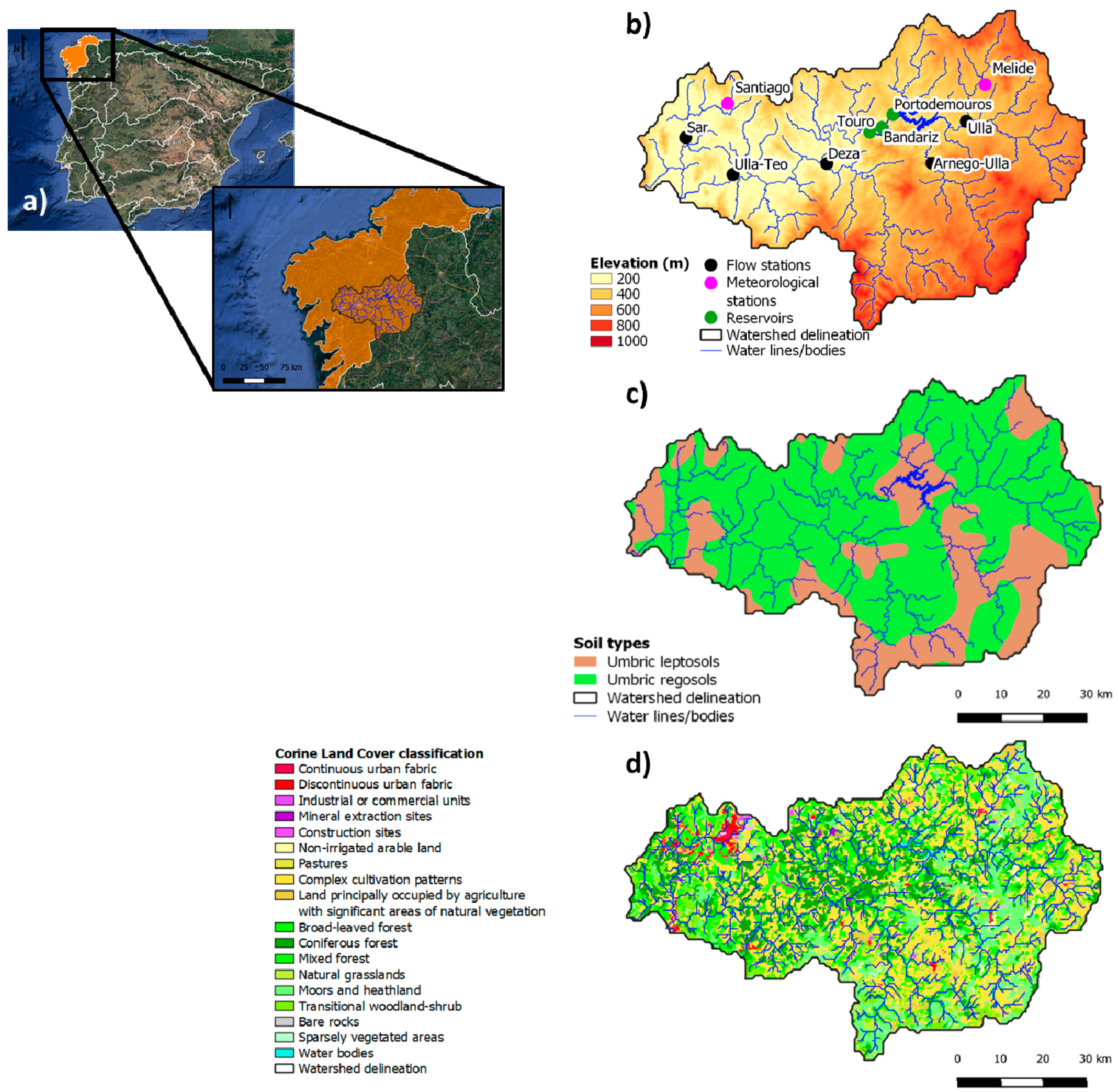
The study area was the watershed of the Ulla River, Galicia, northwestern Spain (Figure 1). The Ulla River watershed has an area of 2803 km2 [28]. Its origin is in Fonte de Ulloa, Monterosso municipality, at a level of about 600 m, and the main watercourse has a bed length of 142 km, crossing 19 counties. The maximum and minimum elevations are 1160 m and −0.75 m, respectively. According to the Köppen-Geiger classification, the climate in the region is a Mediterranean warm summer climate (Csb). The average annual temperature is 12 °C, ranging from 7 °C in February to 18 °C in August. The annual precipitation is 1100 mm, occurring mainly from October to May. The dominant soil units are Umbric Leptosols and Umbric Regosols, occupying 69% and 31% of the area, respectively [29]. The main land uses are forest and semi natural areas and agricultural areas, covering 57.2% and 40.3% of the watershed, respectively [30].
The watershed has a population of about 150,000 inhabitants, mainly located in the cities of Santiago de Compostela, Estrada, Lalín, and Padrón. The Ulla River further includes three reservoirs, namely, Portodemouros, Touro, and Bandariz (Figure 1). Portodemouros has a total capacity of 297 hm3, while Bandariz and Touro are smaller, storing 2.74 hm3 and 3.78 hm3, respectively. The reservoirs are mainly used for energy production and flood control. The three reservoirs function together, with Bandariz and Touro being used to uniformize turbinated flows in Portodemouros during peak times, reducing its impact in downstream areas.
2.2. Model Description
The MOHID-Land model [16,27] is an open source hydrological model; the code can be accessed from an online repository (github.com/Mohid-Water-Modelling-System/Mohid). MOHID-Land simulates the water cycle considering four compartments or mediums: atmosphere, porous media, soil surface, and river network. The atmosphere is not explicitly simulated but provides data necessary for imposing surface boundary conditions that may be space and time variant. The water moves between the remaining mediums based on mass and momentum conservation equations that are computed using a finite volume approach. MOHID-Land is thus a physically based, fully distributed model using an explicit algorithm with a variable time step. The time step is maximum during dry seasons and minimum when fluxes increase.
The simulated domain can be discretized by a regular grid, quadrangular or rectangular, in the surface plane, and by a cartesian coordinate system in the vertical direction. Thus, the surface land is described using a 2D horizontal grid while the porous media is a 3D domain, which includes the same horizontal grid on the surface complemented with a vertical grid with variable thickness layers. The river network is a 1D domain defined from a digital terrain model (DTM). The water lines of the drainage network are then delineated by linking surface cell centers (nodes) together.
2.2.1. Infiltration
The MOHID-Land model includes three options to compute soil water infiltration. The infiltration rate (i, LT−1) can be first estimated according to Darcy’s law, as follows:
where Ksat is the saturated soil hydraulic conductivity (LT−1), h is the soil pressure head (L), and z is the vertical space coordinate (L).
The infiltration rate can also be calculated according to the Green and Ampt method [31]:
where t is the time (T), D0 is the soil water diffusivity (L2T−1), and Δθ is the difference between the volumetric water content in the wetted region (θ0) and soil initial conditions (θi) (Δθ = θ0 − θi, L3L−3). Soil water diffusivity can then be calculated as:
where K0 is the hydraulic conductivity of the wetted region (LT−1), and Δh is the difference between the matric head in the wetted region (h0) and at the moving front (hF) (Δh = h0 − hF).
Finally, the SCS runoff curve number (CN) method [32] can be further used to estimate the infiltration rate. In this method, infiltration water is the amount of water not removed by surface runoff, entering the soil at a rate computed from the ratio between the amount of water available for infiltration and the time step. The surface runoff is first calculated as follows:
where Q is the runoff (L), p is the rainfall (L), S is the potential maximum retention (L) after runoff begins, and Ia is the initial abstraction (L). Initial abstraction considers all losses before runoff begins, as water retained in surface depressions, water intercepted by vegetation, evaporation, and infiltration, and is calculated as:
The S parameter is related to soil properties and land use through the curve number (CN):
The CN values may range between 0 and 100 (-). Higher values of CN are related with more impermeable soils and, consequently, with higher runoff values. In MOHID-Land, the user can define average curve number values (CNII). However, because runoff is affected by soil moisture before a precipitation event, these average values are adjusted for dry (CNI) and wet (CNIII) conditions. The adjustment of the CNII values considers the comparison of the accumulated precipitation during the last five days with predefined thresholds. Under dry conditions, CN values will then decrease while under wet conditions CN values will increase. Nonetheless, it is important to note that, in MOHID-Land, the amount of water in Ia may not fully infiltrate if the soil is saturated, being transformed back to surface runoff and summed to Q in Equation (4).
2.2.2. Surface Flow
Surface flow is computed by solving the Saint-Venant equation in its conservative form, accounting for advection, pressure, and friction forces:
where Q is the water flow in the river (L3T−1), A is the cross-sectional flow area (L2), g is the gravitational acceleration (LT−2), v is the flow velocity (LT−1), H is the hydraulic head (L), n is the Manning coefficient (TL−1/3), Rh is the hydraulic radius (L), and subscripts u and v denote flow directions. In the drainage network, surface flow is solved for one direction (1D domain) considering the water lines obtained from the DTM. The cross-sections in the nodes of the river network are defined by the user. Outside the drainage network, surface flow results from the amount of water that does not infiltrate or ascends by capillarity and is solved on a 2D domain considering the directions of the horizontal grid. Water exchanges between the soil surface and the drainage network are computed according to a kinematic approach, neglecting bottom friction, and using an implicit algorithm to avoid instabilities.
2.2.3. Porous Media
The movement of infiltrated water in the porous media is computed by the Richards equation:
where θ is the volumetric water content (L3L−3), xi represents the xyz directions (-), K is the hydraulic conductivity (LT−1), and S is the sink term representing root water uptake (L3L−3T−1). The soil hydraulic properties are described using the van Genuchten Mualem functional relationships [33,34]:
where Se is the effective saturation (L3L−3), θr and θs are the residual and saturated water contents, respectively (L3L−3), Ksat is the saturated hydraulic conductivity (LT−1), α(L−1) and η (-) are empirical shape parameters, m = 1 − 1/η, and l is a pore connectivity/tortuosity parameter (-). In MOHID-Land, the relation between the horizontal and vertical hydraulic conductivities is defined by a factor (fh = Khor/Kver) that can be adjusted by the user. The model uses the Richards equation in the whole subsurface domain and simulates saturated and unsaturated flow using the same grid. A cell is considered saturated when moisture is above a threshold value (e.g., 98%) defined by the user. When a cell reaches saturation, the model uses the saturated conductivity to compute flow and the pressure becomes hydrostatic, corrected by friction. This procedure eases the implementation of the model and simplifies its use at an annual scale. The penalty is the time step that during the wetting period must be shorter to guarantee stability. The constraint is minimized using parallel computing. The water fluxes between the porous media and the drainage network are also driven by the pressure gradient in the interface of these two mediums.
2.2.4. Root Water Uptake
Root water uptake considers the weather conditions and soil water contents. The reference evapotranspiration rates (ETo, LT−1) are first computed according to the FAO Penman–Monteith method [35]. Crop evapotranspiration rates (ETc, LT−1) are then obtained from the product of ETo and a single crop coefficient (Kc). The Kc is imposed, with the model either assuming a constant value representing the average characteristics of each vegetation type over the entire growing season as well as average effects of evaporation from the soil [27] or a crop stage-dependent value as used in Allen et al. [35]. Advantages and limitations of these approaches are discussed in Canuto et al. [27].
The ETc values are partitioned into potential soil evaporation (Ep, LT−1) and crop transpiration (Tp, LT−1) as a function of the simulated leaf area index (LAI, L2 L−2) [36]:
where λ is the extinction coefficient of radiation attenuation within the canopy (-). The LAI values are simulated using a modified version of the EPIC model [37,38], considering the heat units for the plant to reach maturity, the crop development stages, and crop stress. Additional details can be found in Ramos et al. [17].
Root water uptake reductions, i.e., Tp reductions, are finally computed using the macroscopic approach proposed by Feddes et al. [39], as follows:
where Ta is the actual transpiration rate (Ta, LT−1) and α is a prescribed dimensionless function of h (0 ≤ α ≤ 1) limiting Tp over the root zone in the presence of depth-varying stressors, such as water stress [40,41]. According to the linear model proposed by Feddes et al. [39], root water uptake is maximum when the pressure head is between h2 and h3, has a linear reduction when h > h2 or h < h3, and becomes zero when h < h4 and h > h1 (subscripts 1−4 denote different threshold pressure heads). Finally, the actual soil evaporation (Ea, LT−1) is calculated from Ep values by imposing a pressure head threshold value [42].
2.3. Model Set-Up (Reference Simulation)
The MOHID-Land model was applied to the study area using a constant horizontally spaced grid in the eastern and northern directions (215 columns × 115 rows), with origin on 42.468498° N and 8.801326° W, and a resolution of 0.005° (≈500 m). The DTM was provided by the European Environment Agency (EU-DEM) [43], with a resolution of approximately 30 m (0.00028°). This DTM is a hybrid product based on the Shuttle Radar Topography Mission (SRTM) and the Advanced Spaceborne Thermal Emission and Reflection Radiometer (ASTER) Global Digital Elevation Model (GDEM) data fused by a weighted averaging approach.
The drainage network was derived from the DTM. The geometry of the river cross-sections was defined according to Andreadis et al. [44]. This database relates the drained area in each node to the top width and depth of the cross-section at that node (Table 1). All cross-sections were considered rectangular, with bottom width equal to the top width. For the nodes with intermediate drainage areas, the dimensions of the cross-section were linearly interpolated from the upper and lower classes defined in Table 1. The Manning coefficient was set to a constant value of 0.035 s m−1/3 for the entire drainage network (the model does not allow setting up different values along the river network).
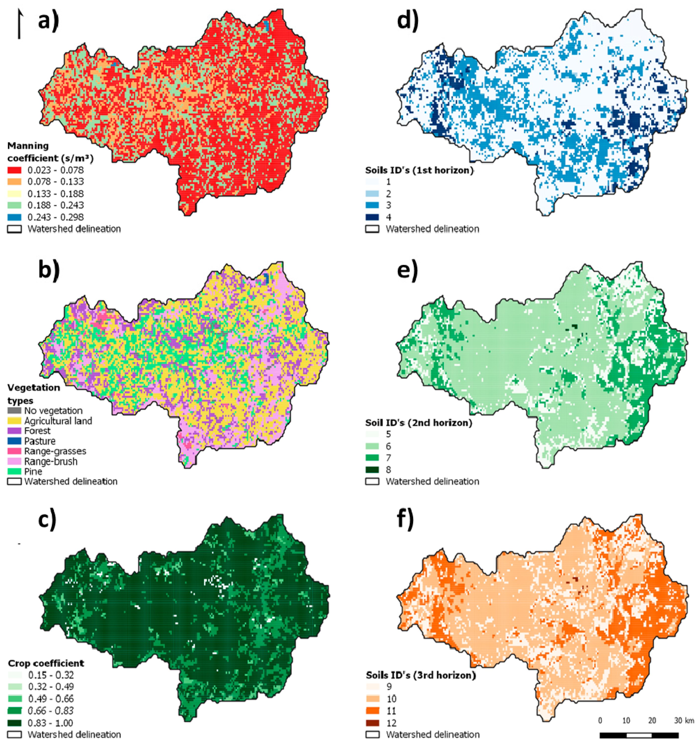
Corine Land Cover [29] data with a resolution of 100 m were used to identify land use. For each land use, the vegetation type and respective Manning’s coefficient were defined. Vegetation type was defined according to MOHID’s vegetation database, while the Manning’s coefficients were defined according to Pestana et al. [45]. The Kc values were set based on vegetation type. As mentioned earlier, these coefficients represent empirical average values for the growing season and are not stage dependent as in Allen et al. [35]. The resulting interpolation to the MOHID’s simulation domain (Figure 2) showed a variation for the Manning coefficient from 0.023 to 0.298 s m−1/3 while the Kc values varied from 0.15 to 1.0 (Figure 2).
The soil domain was divided into six grid layers, with a thickness from the surface to the bottom layers of 0.3, 0.3, 0.7, 0.7, 1.5, and 1.5 m (vertical grid). On the other hand, the soil profile was characterized by three horizons: 0 to 0.6 m, 0.6 to 2.0 m, and 2.0 m to the soil bottom. Thus, the first horizon included the first two grid layers, the second horizon included the two middle grid layers, and the third horizon consisted of the two bottom layers of the vertical grid domain. The soil depth in each cell was estimated considering the cell slope, with flat areas approximating a maximum predefined value while sloped areas approached a minimum. These maximum and minimum soil depths were defined as 5.0 and 0.1 m, respectively. Soil data were extracted from the multilayered European Soil Hydraulic Database [46]. This database includes the Mualem–van Genuchten hydraulic parameters for the whole of Europe at a resolution of 250 m. Information is provided at 0, 0.05, 0.15, 0.3, 0.6, 1.0, and 2.0 m depths. For the present application, the 0.3 m layer was used to characterize the first horizon, the 1.0 m layer was used for the second horizon, and the 2.0 m layer was used for the bottom horizon. Figure 2 shows the spatial distribution of soil data in the Ulla watershed while Table 2 presents the corresponding Mualem–van Genucthen parameters. The fh parameter, which relates the horizontal and vertical hydraulic conductivities, was set to 10. For the initial conditions, the soil was assumed as saturated for 95% of the profile (from the bottom to the surface), while the soil water content in the vadose zone was set to field capacity. Soil water infiltration was computed following the Darcian approach (Equation (1)).
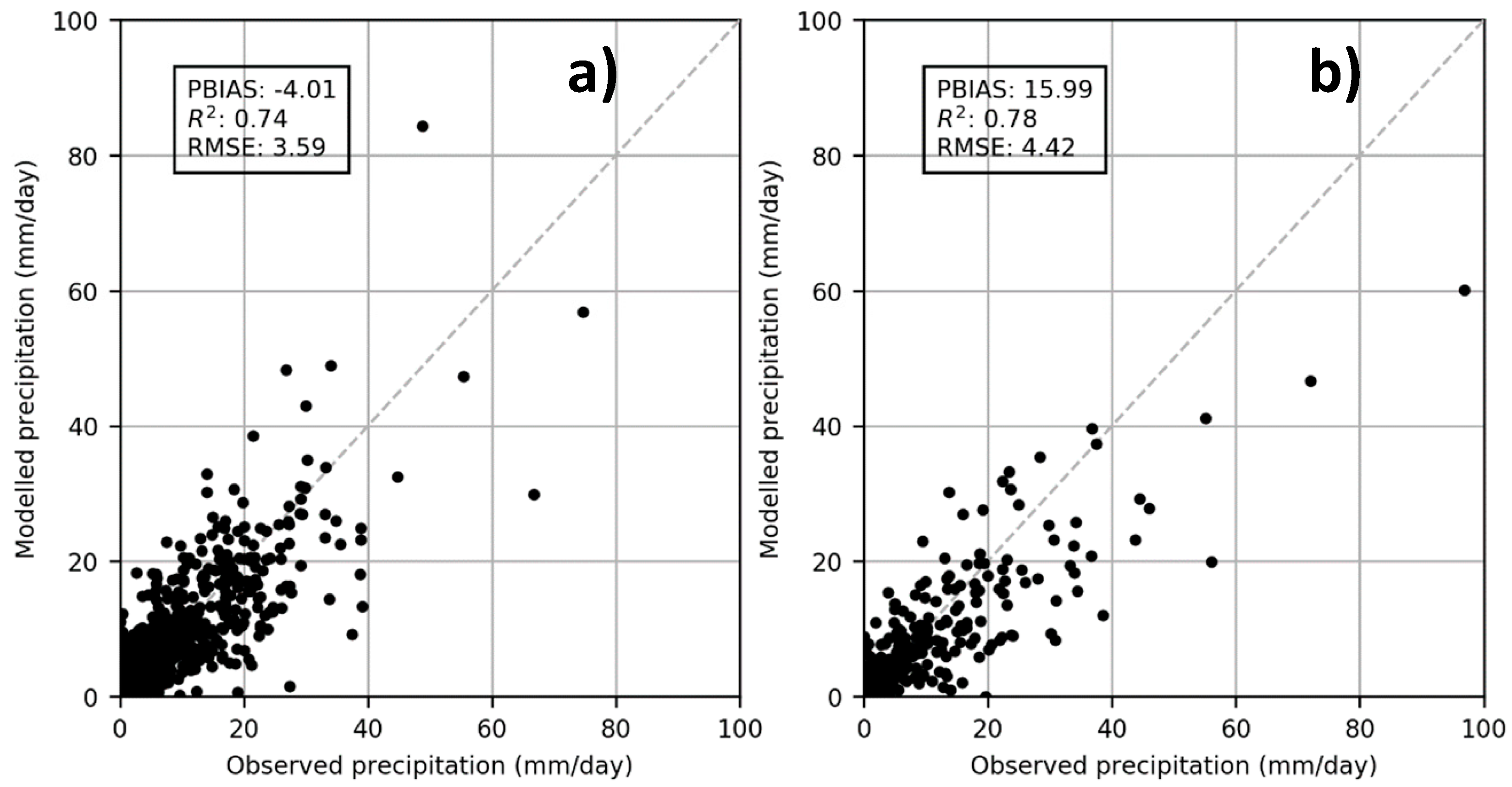
Meteorological data were extracted from the ERA5-Reanalysis dataset [47]. This dataset provides several gridded meteorological parameters with an hourly timestep and with a resolution of 0.28125° (31 km). The variables used were the u and v components of wind velocity at 10 m height, dewpoint temperature and air temperature at 2 m height, surface solar radiation downwards, surface pressure, total cloud cover, and total precipitation. The ERA5 precipitation data were first validated through comparison with measured values obtained at Melide and Santiago meteorological stations (Figure 1). For the Melide station, a comparison was conducted from 1 January 2008 to 31 December 2012, resulting in a coefficient of determination (R2) of 0.74 (Figure 3). For the Santiago station, that period was from 1 January 2016 to 31 December 2017, with the R2 value reaching 0.78. The ERA5 data were then interpolated to the case study grid.
2.4. Sensitivity Analysis
The computational cost of one single run with the MOHID-Land model made it impossible to carry out thousands of runs to perform a global and detailed sensitivity analysis. Thus, a local sensitivity analysis was performed by modifying selected MOHID-Land parameters and processes one at the time and evaluating their impact on river flow. The respective flow-duration curves, which express the exceedance probability of a certain flow [48], were then compared against the reference simulation. A sensitivity index was finally computed following the methodology proposed by Ranatunga et al. [7].
The simulated river flows at a specific location were arranged in a descending order and ranked from 1 to N with the exceedance probability (frequency of occurrence) being given as follows:
where F is the exceedance probability (expressed as a percentage of time a flow value is equaled or exceeded), R is the rank, and N is the total number of flow values resulting from the simulation. The flow duration curve is thus the graphical representation of flow values and the corresponding F values. The flow duration curves were then divided into five zones based on the percentage exceedance as shown in Figure 4. Flows with an F value from 0 to 10% were considered high flows; 10 to 40% corresponded to moist conditions; 40 to 60% corresponded to mid-range flows; 60 to 90% corresponded to dry flows; and 90 to 100% corresponded to low flows [7].
The sensitivity index (SI) aimed at measuring the relative influence of the analyzed parameters/processes on river flow. This index results from the normalization of the root mean square error (RMSE) by dividing the error of the estimate of each simulated scenario by the range of flow values of the reference simulation:
where Qiref is the flow of the reference simulation on day i, Qisim is the flow of the analyzed simulation on day i, Qmaxref and Qminref are the maximum and minimum flow values of the reference simulation in the respective flow classes, and p is total number of flow daily values in the same flow class. A larger influence of a parameter/process on watershed hydrology is represented by higher values of SI, while lower values of SI mean a lower influence of the analyzed parameter/process.
Model simulations were performed from 1 January 2008 to 31 December 2012 (five years). The first four months of simulations were considered as the warm-up period and were not included in the analysis of the results. Flows were analyzed at a daily scale. Due to MOHID-Land’s high computational requirements and having as the ultimate goal the calibration of Ulla River watershed, the sensitivity analysis focused on a single variation of the selected parameters/processes, illustrating the impact of those variables on model performance. The analyzed parameters/processes as well as the variations imposed on model inputs were defined based on previous calibrations of the MOHID-Land model for different watersheds [22,25,26,27]. Additionally, the calibration processes performed on similar physically based models were also considered [49,50,51,52,53,54]. Thus, sixteen parameters/processes influencing water dynamics at the catchment scale were analyzed:
- The resolution of the simulation grid was modified from 0.005° (≈500 m) used in the reference simulation to 0.01° (≈1000 m; 140 columns × 100 rows) (simulation 1, S1).
- The DTM was changed from the EU-DEM (30 m) to the one provided by the National Geographic Institute of Spain, with a resolution of 5 m [55]. The new DTM was interpolated to the simulation grid, with the model also delineating a new catchment area and drainage network based on that input (S2).
- The effect of cross-section geometry on river flow was assessed in two simulations. In one (S3), the top and bottom widths were increased by 25% (i.e., larger river) while the depth and the shape of the cross-section remained the same. In the other (S4), the river depth was increased by 100%, while the top and bottom widths and the shape of the cross-section were maintained as in the default simulation. Table 1 shows the variations introduced to those parameters per drainage area.
- The Ksat value of each cell was multiplied by a factor of 10 while fh was maintained (S5). As a result, the horizontal hydraulic conductivity was also modified since fh = Khor/Kvert.
- The fh value was analyzed in a separate test by changing this parameter from 10, in the reference simulation, to 20 (S6). The Ksat,vert values were the same as in the default scenario, meaning that a change in fh led to an increase in the Khor.
- The number of layers in the vertical grid increased from 6 to 12 as defined in Table 3 (S7), thus decreasing the thickness of the layers when compared with the reference simulation.
- The soil depth also increased from 5 to 10 m (S8), with the number of layers in the vertical grid increasing from six to nine (Table 3).
- The surface Manning coefficients increased by 50% when compared with the reference simulation (S9).
- The channel Manning coefficient also increased from 0.035 s m−1/3 to 0.0525 s m−1/3, corresponding to a 50% increase (S10).
- The SCS curve number method was used to compute runoff and soil water infiltration as an alternative to Equation (1) (S11). The CN values were defined for each grid cell according to the soil type and land cover. The hydrologic soil groups (HSGs) were extracted from the HYSOGs250 m dataset [56], which derived that information from the soil texture classes and depth to bedrock available in the SoilGrids250 m product [57]. That information was then merged with Corine Land Cover [29] data following the United States Department of Agriculture [58] guidelines to derive the CN values. Figure 5 presents the CN values adopted in this study. Additionally, changes in the CN values were also assessed by decreasing the values set in S11 by 25% (S12).
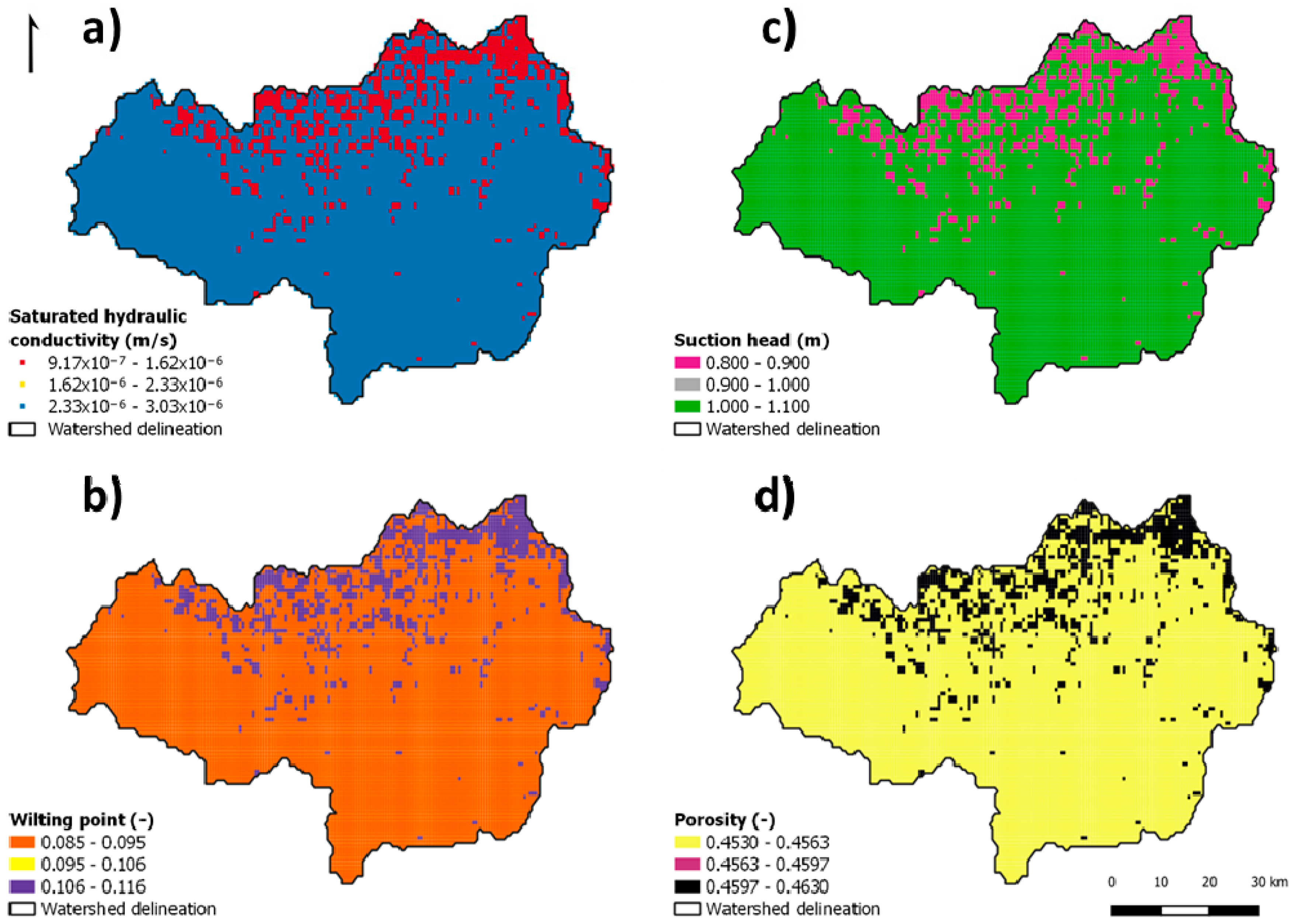
- The Green and Ampt infiltration method was now used as an alternative to Equation (1) (S13). The MOHID-Land model needed the values of Ksat,ver, suction head, porosity, and wilting point in each cell as inputs (Figure 6). These inputs were obtained by combining the information available in the LUCAS database [59] with data from Rossman [60], who related the soil texture classes with the soil hydraulic characteristics.
- The importance of the porous media and vegetation growth processes for river flow results were investigated in three separate simulations. Firstly, vegetation growth processes were deactivated (S14), meaning that no evapotranspiration occurred in the catchment area. Secondly, both the porous media and vegetation growth processes were deactivated (S15). In the absence of porous media, the SCS CN method was used to compute the partitioning of rainfall data between surface runoff and infiltration. Infiltration water was then lost to the system since soil porous processes were not considered. The CN values presented in Figure 5 were adopted for this analysis. Lastly, both porous media and vegetation growth processes remained deactivated, but the CN values were reduced by 25% (S16) as in S12.
The time required for MOHID-Land to compute each simulation was also quantified. The average, maximum, and minimum time (in seconds) required to complete each day of simulation were compared for all scenarios. This information was critical to understand which parameters/processes would improve computational speed during model calibration/validation.
2.5. Model Calibration/Validation
Based on results from the sensitivity analysis, the following parameters/processes were modified from those adopted in the reference simulation during model calibration/validation: the vertical hydraulic saturated conductivity (Ksat,ver); the relation factor between the horizontal and vertical hydraulic conductivities (fh); and the dimensions of the cross-sections in the river network. Model calibration consisted of modifying these parameters one at a time, and adjusting them by trial-and error, until deviations between model simulations and flow measurements at Sar, Ulla, Arnego-Ulla, and Deza hydrometric stations (Figure 1) were minimized. Validation was then performed by simply comparing model simulations using the calibrated parameters with flow measurements at the same hydrometric stations. The Sar, Ulla, Arnego-Ulla, and Deza hydrometric stations were selected because their data describe the natural flow regime of the Ulla watershed, which was obtained from Augas de Galicia [61]. The Ulla-Teo station (Figure 1) was under the influence of reservoir management and therefore its data were not considered for evaluating model performance. Model simulations were carried out from 1 January 2008, to 31 December 2017 (10 years). The first four months were considered as the warm-up period, while the period between 1 May 2008 and 31 December 2012 was considered for calibration. The validation period was defined between 1 January 2013 and 31 December 2017.
Different goodness-of-fit tests were considered for assessing model performance, including the Nash and Sutcliffe model efficiency (NSE), the percent bias (PBIAS), the RMSE-observation standard deviation ratio (RSR), and the coefficient of determination (R2). The NSE [62] was computed as:
where Qiobs is the observed flow on day i, Qisim is the simulated flow for day i, Qmeanobs is the observed mean flow for the period under consideration, and p is the total number of days in that same period. The NSE is used to assess the relative magnitude of residual variance compared to the measured data variance and it ranges between −∞ and 1.0, being 1.0 the optimal value. Values between 0.0 and 1.0 are classified as acceptable levels of performance, and values ≤ 0.0 indicate that the mean observed value is a better predictor than the simulated value.
The PBIAS is a statistical parameter that measures the average tendency of the simulated data to be larger or smaller than their observed counterparts, and was computed as follows:
The optimal value of PBIAS is 0.0 and low-magnitude values indicate accurate model simulation. Positive values demonstrate model underestimation while negative values represent model overestimation.
The RSR results from the ratio between the RMSE and the standard deviation of observed values were obtained as follows:
RSR incorporates the benefits of error index statistics and includes a scaling/normalization factor. RSR is equal to 0.0 when RMSE is 0.0, indicating that the variation is residual, and the model is perfect. Thus, low RSR values correspond to low RMSE values and a good model simulation performance.
Finally, R2 describes the degree of collinearity between simulated and measured data and ranges from 0 to 1, with higher values indicating less error variance. This statistical parameter was computed as follows:
According to Moriasi et al. [63], model performance for streamflow can be classified as satisfactory when NSE > 0.50, RSR ≤ 0.70, PBIAS ± 25%, and R2 > 0.5.
3. Results and Discussion
3.1. Impact of Model Parameters/Processes on River Flow
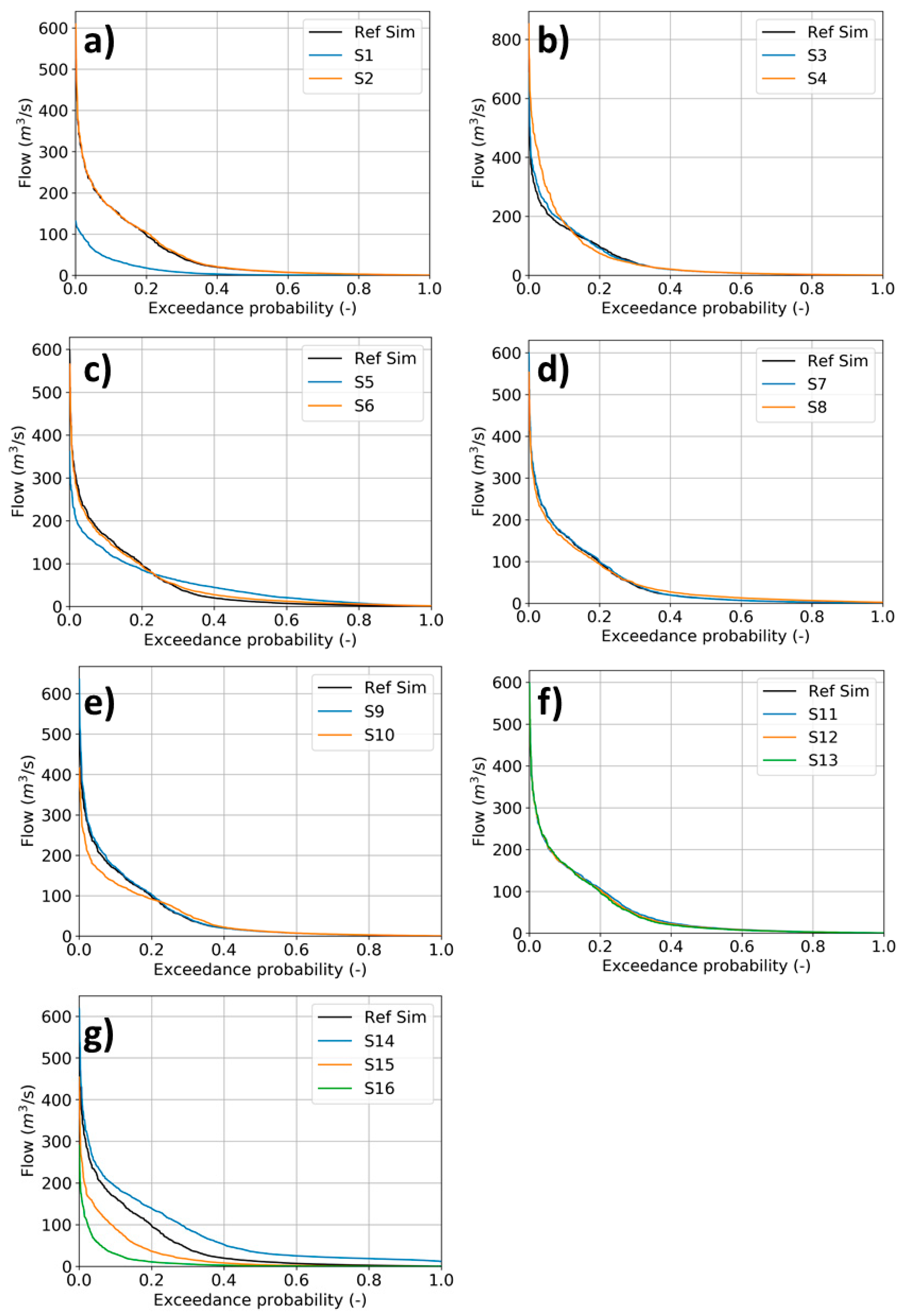
Although flow-duration curves were compared for all flow stations, only results for the Ulla-Teo station (Figure 1) are presented graphically, to limit the number of figures and to maintain consistency. This station was not considered for evaluating model performance because of the influence of reservoir management on river flow. However, its larger drainage area produced the most contrasting differences between the simulation scenarios and the reference simulation, which helped demonstrate model behavior during the sensitivity analysis. Figure 7 shows the flow-duration curves for each simulation included in the sensitivity analysis, while Table 4 and Table 5 present the mean flow and respective SI values for each exceedance probability class.
Decreasing the resolution of the base grid from 500 m (reference simulation) to 1000 m (S1) had a substantial impact on river flow, with mean values decreasing between 71% and 97% in all ranges of the flow-duration curve (Table 4). That was also visible in the SI values, which ranged from 0.42 to 0.93 (Table 5). These results showed that setting up the base grid, which basically defined how detailed the study area would be represented, was an important step for accurately simulating river flow at the catchment scale. A more detailed grid led to a more dynamic watershed than when using a coarser one. These results contrast with Sreedevi and Eldho [54], who, after testing three grid sizes (4000, 2000, and 1000 m), found no scale dependency on streamflow generation values using the SHETRAN model. Nevertheless, the use of a coarser resolution grid in the Ulla River watershed had a contrasting result at the hydrometric stations located in the river heads above 600 m (Sar, Arnego-Ulla, and Deza). In those locations with a drainage area smaller than at Ulla-Teo, the coarser steeper slopes in the DTM ended up promoting surface runoff and higher flow peaks, which eventually disappeared by the time the iflow reached the Ulla-Teo station.
On the other hand, for the same resolution grid (500 m), results with a more detailed DTM (S2) did not differ much from the reference simulation (Table 4 and Table 5). The use of high-resolution data in coarse scale applications seems thus to be irrelevant when not accompanied by a base grid also with greater resolution to be able to consider such detailed information. Yet, improvements n streamflow simulations using more detailed grids and DTMs can only go so far, as shown by Pieri et al. [50]. These authors found no statistically significant differences in the accuracy of DTMs varying between 10 and 2 m resolution when simulating streamflow and sediment yield using the WEPP model in a considerably smaller basin than the Ulla River catchment (the Centonara catchment in northern Italy, 1.92 km2). Also, Zhang et al. [51] and Nazari-Sharabian et al. [53] showed the influence of the DTM resolution on the calibration of streamflow simulations using different physically based models.
Increasing the width (S3) and depth (S4) of the cross-sections (i.e., the river network) promoted higher river flow in all the exceedance intervals except for the moist conditions (Q10−40), where it slightly decreased (Figure 7). The largest increase was in the higher flow class (Q0−10), i.e., the flow peaks, with S3 and S4 leading to an increase of the mean flow by 11% and 39%, respectively (Table 4). This was explained by the fact that increasing the dimensions of the cross-sections meant that the boundary between the riverbed and the porous media would also increase, promoting water exchanges between these two mediums, mainly from the porous media to the riverbed. However, only S4 resulted in higher SI values in the extremes of the flow duration curve, reaching 0.29 for the Q90−100 class and 0.26 for the Q0−10 class.
The increase in Ksat,ver (S5) and fh (S6) led to a rise of river flow values in the mid-range (Q40−60), low (Q60−90), and dry (Q90−100) classes of the flow duration curve, which varied from 48% to 188% when compared with the reference simulation. On the other hand, flow values in the Q0−10 range (high flows) showed a decreasing trend while the Q10−40 class (moist condition) remained basically unchanged. Thus, the increase in those parameters promoted the infiltration process (exchange between the surface and the porous media), the faster movement of soil water (subsurface flow), and the exchange between the porous media and river sections. Higher subsurface flows caused the water to allocate to the baseflow instead of generating flow peaks, increasing the mean values in the lower classes of the flow-duration curve. As a result, the SI values were notoriously higher in the lower classes of the flow duration curve (Q40−60 to Q90−100), reaching values from 1.20 to 1.52 in S5 and from 0.48 to 1.52 in S6 (Table 5) due to the increasing baseflow. Note that a scaling factor of 10 was considered for varying Ksat,ver, in line with previous calibrations of this parameter performed by Canuto et al. [27] in the Guadiana catchment, Iberian Peninsula. However, this parameter is known to be one of the most variable in nature, being affected by soil physical, chemical, and biological properties. There is also the fact that Tóth et al. [46] maps were developed from a database containing measurements of this parameter carried out in the laboratory on samples of limited size, with issues related to their representativeness being often raised when describing actual flow conditions, transport, and reaction processes occurring at the field/catchment scales due to limitations in the porous medium continuum [64,65]. Similarly, a scaling factor of 20 was considered in this application for fh. The literature is far less rich on variations of this parameter since it is specific to the MOHID-Land model. Yet, fh has been found to vary between 3.0 [27] and 25.0 [25]. The latter was used to fit simulated streamflow to measurement values in the Alegria River watershed, northern Spain. Thus, different scaling factors could have been here considered for Ksat,ver and fh, but results would not differ much since the main point was to identify which hydrological processes would be affected by these parameters.
The influence of vertical discretization (S7) on river flow was practically null. This explains the relatively coarse discretization of the vertical grid in existing applications of the MOHID-Land model at the watershed scale [22,25,26,27]. These studies reported vertical grids varying from 7 to 12 layers when describing soil profiles reaching 8 to 30 m depth. More detailed grids would have increased the computational burden with no practical benefit for model performance. Nonetheless, those numbers contrast with the one-dimensional application presented in Ramos et al. [17], who used 100 grid cells with 0.02 m thickness each to describe soil water dynamics in a soil profile with 2 m depth and respective interactions between the vadose zone and a shallow groundwater table. On the other hand, a deeper soil profile (S8) led to an increase in the lower exceedance probability classes of the flow-duration curve (Q40−60, Q60−90 and Q90−100) from 53% to 289% (Table 4), resulting in higher SI values in those classes (0.52 to 2.71). The increase in soil depth represented a larger volume of water stored below the surface, at depths (bottom profile) that were not affected by evapotranspiration. This water stored at deeper depths became thus an additional resource for exchanges between the porous media and the river network, leading to higher baseflow.
The impact of modifying the surface’s Manning coefficients was small (S9). This agreed with Canuto et al. [27], who considered this parameter in the calibration of streamflow simulations in the Guadiana basin, but changes to the model’s default values ended up being only minor. Changing the channel’s Manning coefficient (S10) resulted in a decrease of the mean flow in the Q0−10 class by 23% and an increase in the Q90−100 class by 10% (Figure 7, Table 4). Increasing the roughness and, consequently, the friction between the water and the surface led to a decrease in flow velocity. The infiltration process was then promoted, causing an increase in baseflow and a reduction of the flow peaks. Nonetheless, the SI values were always smaller than 0.14, which show the reduced influence of this parameter in the generation of streamflow.
The use of the SCS CN method (S11) promoted the increase in mean flow values for the moist (Q10−40), mid-range (Q40−60), and dry flow classes (Q60−90) by 8%, 19%, and 14%, respectively, when compared with the reference simulation (Table 4). Flow in the Q40−60 class also corresponded to the highest SI value (0.20; Table 5). Reducing the CN values of all grid cells by 25% (S12) naturally led to less runoff, with the mean flow values for the same classes referred to above being 3%, 9%, and 6% higher than in the reference simulation while in the Q90−100 class they were lower by 6%. The use of the Green and Ampt method as an alternative to Equation (1) had no real impact on river flow. Obviously, future works need to analyze the sensitivity of the MOHID-Land model to inputs used for computing soil water infiltration with this method. Notwithstanding, the MOHID-Land model offers analytical, semi-analytical, but also empirical solutions for modeling a key process in the hydrological cycle, which can be selected depending on the complexity of users’ applications.
Finally, the deactivation of vegetation (S14) and porous media (S15) modules produced a strong modification of the flow-duration curve at the Ulla-Teo station (Figure 7), which was expected since most processes included in the reference simulation were disregarded. Ignoring the evapotranspiration process in the catchment (S14) led to an increase in the mean flow in all intervals of the flow duration curve, particularly in the mid-range (Q40−60), dry (Q60−90), and low flow (Q90−100) classes (Table 4). Flow in the Q90−100 class also returned the highest SI value of 14.32 (Table 5). Without the main driver for soil water dynamics, soil water contents as well as exchanges between the porous media and the river network simply increased, promoting mainly baseflow. The porous media module was responsible for the occurrence of subsurface flow and baseflow. This constituted a major component in the water budget of the Ulla River catchment. Disregarding this module naturally led to a decrease in the mean river flow values in all classes of the flow-duration curve because the infiltrated water simply disappeared from the system. With the reduction of the CN values by 25% (S16), that drop was even higher (Table 4).
3.2. Impact of Model Parameters/Processes on Model Time Consumption
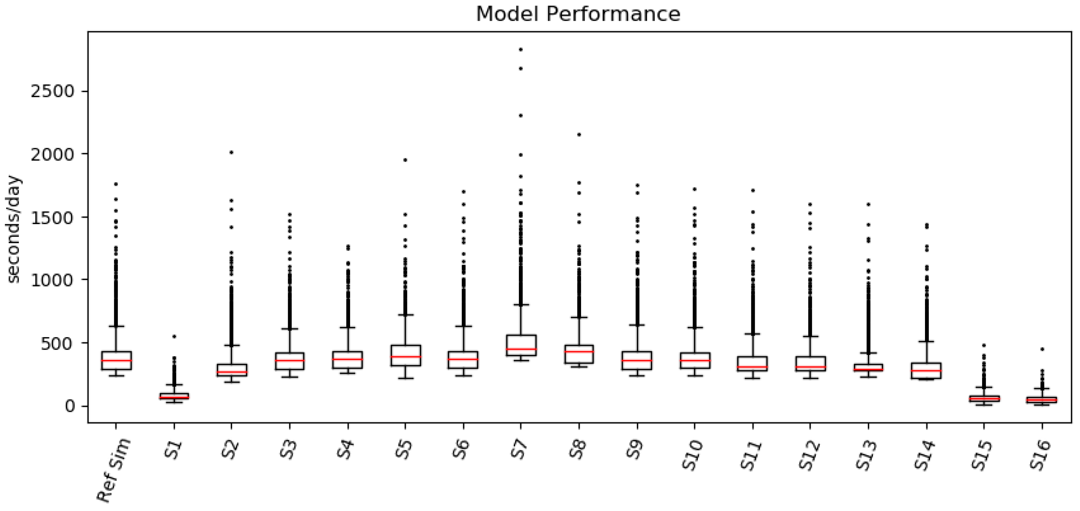
Figure 8 presents the boxplot of the time required for MOHID-Land to compute each day of the simulations considered in the sensitivity analysis, while Table 6 summarizes those results by presenting the minima, mean, and maxima values. The fastest computation time was naturally obtained by running the simplest applications, i.e., S2 with the coarser grid resolution of 1000 m, and S15 and S16 without considering the porous media processes. The former can be explained by a simulation grid four times smaller than the one in the reference simulation, substantially decreasing the calculations needed to run the simulation, and the latter by disregarding subsurface flow, with MOHID-Land distancing from its physically based nature and relying on a more empirical basis. On the other hand, the longest simulation performance was achieved with a more detailed vertical grid domain (S7). The higher number of vertical layers increased the calculations related to the porous media processes, with the model spending more time to perform the simulation. However, as showed earlier, this had no impact on river flow. All other simulations presented a similar computation time, with no real influence on the number of days (seven days) the reference simulation took to run.
3.3. Prediction of River Flow in the Ulla River Watershed
Figure 9 visually compares the measured and modeled river flow values at the Sar, Ulla, Arnego-Ulla, and Deza hydrometric stations during the calibration (2008−2012) and validation (2013−2017) periods. The respective goodness-of-fit indicators are presented in Table 7. These results were obtained after modifying Ksat,ver, fh, and the dimensions of the cross-sections in the river network defined for the reference simulation. The Ksat,ver values for each soil horizon in Table 2 were multiplied by a scaling factor of 10, similarly as performed in the sensitivity analysis. The fh value was then automatically updated since this parameter represents the relation between horizontal and vertical conductivities in each cell. The dimensions of the cross-sections were defined as shown in Table 1 and consisted of increasing river depth and interactions between the porous media and the river network. Thus, by modifying these parameters, the calibration process mainly focused on increasing baseflow in the Ulla River watershed.
The R2 values varied from 0.56 to 0.75 during the calibration period and from 0.76 to 0.85 during the validation period (Table 7), showing that the model could explain most of the variability of the measured data in all hydrometric stations. The errors of the estimates were relatively small as shown by the low RSR values obtained at the different stations during both simulation periods (RSR ≤ 0.67). On the other hand, the PBIAS values showed some underestimation of measured values at the Sar hydrometric station (PBIAS ≤ 16.09%), and some overestimation of measured data for the remaining stations (−18.54% ≤ PBIAS ≤ −4.35%). Finally, the NSE values were relatively high in most locations, ranging from 0.55 to 0.84 during both periods, indicating that the residual variance was much smaller than the measured data variance. These indicators are comparable with the best flow estimates under natural regimes in Canuto et al. [27], with model predictions for the Ulla River watershed being considered extremely satisfactory if Moriasi et al. [63] guidelines are considered.
Despite the good statistical results, Figure 9 further showed the difficulty of the MOHID-Land model in predicting the highest flow peaks in the Ulla River watershed. This was attributed to the precipitation inputs provided by the ERA5 dataset, which also failed to represent higher precipitation values as shown in Figure 3 for the Santiago meteorological station. This tendency was also verified by Hénin et al. [66], who concluded that reanalysis products such as ERA5 present an underestimation of heavy precipitation events. Hence, the amount of water entering the basin during heavy rain events in that dataset was clearly below measured rainfall and proved to be insufficient for the model to reach higher flow peaks. However, the replacement of the ERA5 data by measured values from the different weather stations was not considered as a viable solution to overcome this problem. Rainfall measurements were only available at a daily time step while the ERA5 data have an hourly time step. In the MOHID-Land model, daily measured data are distributed evenly during the day, reducing rainfall intensity rates, which would further reduce or even miss flow peaks. Besides that, one should consider that the model was calibrated for the entire period without special distinction between dry and wet seasons, which could also explain the difficulty for the model to reach peak flows in the Ulla River watershed. One way to overcome the problem from the model point of view would have been to define distinct geometries of the cross-sections per subbasin, and not per drainage area. This would increase model accuracy of river flow predictions at the watershed scale.
4. Conclusions
The MOHID-Land model is a complex, physically based, three-dimensional model used for catchment scale applications. The sensitivity analysis helped to identify the most relevant parameters/processes influencing river flow generation and for accurately modeling baseflow and peak flows. For the application in the Ulla River catchment, the resolution of the simulation grid, the choice of the infiltration method, and the evapotranspiration process were the main factors influencing river flow generation. The soil hydraulic properties, the depth of the soil profile, and the dimensions of the river cross-sections, which basically control the interactions between the porous media and the river, influenced baseflow. On the other hand, peak flows were mostly constrained by the channel’s Manning coefficient, as well as the dimensions of the river cross-sections.
The sensitivity analysis further showed that the use of a too coarse resolution grid as well as the deactivation of the porous media and vegetation processes can compromise the quality of results, which should then be subjected to careful revision. Also, model simulations of soil infiltration considering the Darcian and the Green and Ampt approaches produced very similar outputs, both in terms of river flow values and computational time, meaning that users can choose between the two solutions depending on available data. Finally, the number of layers in the vertical simulation grid can lead to a substantial increase in the time needed to compute model simulations with no effect on river flow predictions. It is also important to note that the sensitivity analysis focused on just a few input parameters/processes used in MOHID-Land for simulating river flow at the watershed scale. Others should also be considered in future analysis, namely, the remaining soil hydraulic parameters, the crop coefficients, as well as the parameters used for water quality modeling.
Nevertheless, the MOHID-Land model is a powerful tool for simulating river flow at a daily scale in areas under natural flow regimes. This was demonstrated in simulations of the Ulla River flow at four locations, with comparisons between model predictions and measured values returning R2 ≥ 0.56, RSR ≤ 0.67, and NSE ≥ 0.55. These same simulations showed a clear underestimation of river flow peaks, which was attributed to the quality of the ERA5 dataset and the misrepresentation of higher rainfall events.
Author Contributions
Conceptualization, A.R.O.; Formal analysis, A.R.O.; Investigation, A.R.O.; Methodology, A.R.O. and T.B.R.; Software, A.R.O.; Visualization, A.R.O.; Writing—original draft, A.R.O. and T.B.R.; Writing—review & editing, L.S., L.P. and R.N. All authors have read and agreed to the published version of the manuscript.
Funding
This work was supported by FCT/MCTES (PIDDAC) through project LARSyS—FCT Pluriannual funding 2020−2023 (UIDB/50009/2020). The authors also acknowledge project Hazrunoff (UCPM-783208) supported by the Directorate-General for European Civil Protection and Humanitarian Aid Operations. T. B. Ramos was supported by contract CEECIND/01152/2017.
Conflicts of Interest
The authors declare no conflict of interest.
References
- Wheater, H.; Sorooshian, S.; Sharma, K.D. (Eds.) Hydrological Modelling in Arid and Semi-Arid Areas; International Hydrology Series; Cambridge University Press: Cambridge, UK, 2007; pp. 1–4. [Google Scholar]
- Devi, G.K.; Ganasri, B.P.; Dwarakish, G.S. A review on hydrological models. Aquat. Procedia 2015, 4, 1001–1007. [Google Scholar] [CrossRef]
- Sitterson, J.; Knightes, C.; Parmar, R.; Wolfe, K.; Muche, M.; Avant, B. An Overview of Rainfall-Runoff Model Types; U.S. Environmental Protection Agency: Washington, DC, USA, 2017.
- Fatichi, S.; Vivoni, E.R.; Ogden, F.L.; Ivanov, V.Y.; Mirus, B.; Gochis, D.; Downer, C.W.; Camporese, M.; Davidson, J.H.; Ebel, B.; et al. An overview of current applications, challenges and future trends in distributed process-based models in hydrology. J. Hydrol. 2016, 537, 45–60. [Google Scholar] [CrossRef] [Green Version]
- Abbott, M.B.; Bathurst, J.C.; Cunge, J.A.; O’Connell, P.E.; Rasmussen, J. An introduction to the European Hydrological System, Systeme Hydrologique Europeen, “SHE”, 1: History and philosophy of a physically-based, distributed modelling system. J. Hydrol. 1986, 87, 45–59. [Google Scholar] [CrossRef]
- Abbott, M.B.; Bathurst, J.C.; Cunge, J.A.; O’Connell, P.E.; Rasmussen, J. An introduction to the European Hydrological System, Systeme Hydrologique Europeen, “SHE”, 2: Structure of a physically-based, distributed modelling system. J. Hydrol. 1986, 87, 61–77. [Google Scholar] [CrossRef]
- Ranatunga, T.; Tong, S.T.Y.; Yang, Y.J. An approach to measure parameter sensitivity in watershed hydrological modelling. Hydrol. Sci. J. 2017, 62, 76–92. [Google Scholar] [CrossRef]
- Pianosi, F.; Beven, K.; Freer, J.; Hall, J.; Rougier, J.; Stephenson, D.; Wagener, T. Sensitivity analysis of environmental models: A systematic review with practical workflow. Environ. Model. Softw. 2016, 79, 214–232. [Google Scholar] [CrossRef]
- Silva, M.G.; Netto, A.O.A.; Neves, R.J.J.; Vasco, A.N.; Almeida, C.; Faccioli, G.G. Sensitivity analysis and calibration of hydrological modeling of the watershed Northeast Brazil. J. Environ. Prot. 2015, 6, 837–850. [Google Scholar] [CrossRef] [Green Version]
- Shi, Y.; Xu, G.; Wang, Y.; Engel, B.A.; Peng, H.; Zhang, W.; Cheng, M.; Dai, M. Modelling hydrology and water quality processes in the Pengxi River basin of the Three Gorges Reservoir using the soil and water assessment tool. Agric. Water Manag. 2017, 182, 24–38. [Google Scholar] [CrossRef]
- Song, X.; Zhang, J.; Zhan, C.; Xuan, Y.; Ye, M.; Xu, C. Global sensitivity analysis in hydrological modeling: Review of concepts, methods, theoretical framework, and applications. J. Hydrol. 2015, 523, 739–757. [Google Scholar] [CrossRef] [Green Version]
- Sreedevi, S.; Eldho, T.I. A two-stage sensitivity analysis for parameter identification and calibration of a physically-based distributed model in a river basin. Hydrol. Sci. J. 2019, 64, 701–719. [Google Scholar] [CrossRef]
- Christiaens, K.; Feyen, J. Use of sensitivity and uncertainty measures in distributed hydrological modeling with an application to the MIKE SHE model. Water Resour. Res. 2002, 38. [Google Scholar] [CrossRef]
- Hamby, D.M. A review of techniques for parameter sensitivity. Environ. Monit. Assess. 1994, 32, 135–154. [Google Scholar] [CrossRef]
- Doherty, J.; Hunt, R.J. Two statistics for evaluating parameter identifiability and error reduction. J. Hydrol. 2009, 366, 119–127. [Google Scholar] [CrossRef]
- Trancoso, A.R.; Braunschweig, F.; Leitão, P.C.; Obermann, M.; Neves, R. An advanced modelling tool for simulating complex river systems. Sci. Total Environ. 2009, 407, 3004–3016. [Google Scholar] [CrossRef]
- Ramos, T.B.; Simionesei, L.; Jauch, E.; Almeida, C.; Neves, R. Modelling soil water and maize growth dynamics influenced by shallow groundwater conditions in the Sorraia Valley region, Portugal. Agric. Water Manag. 2017, 185, 27–42. [Google Scholar] [CrossRef]
- Ramos, T.B.; Simionesei, L.; Oliveira, A.R.; Darouich, H.; Neves, R. Assessing the impact of LAI data assimilation on simulations of the soil water balance and maize development using MOHID-Land. Water 2018, 10, 1367. [Google Scholar] [CrossRef] [Green Version]
- Simionesei, L.; Ramos, T.B.; Brito, D.; Jauch, E.; Leitão, P.C.; Almeida, C.; Neves, R. Numerical simulation of soil water dynamics under stationary sprinkler irrigation with MOHID-Land. Irrig. Drain. 2016, 65, 98–111. [Google Scholar] [CrossRef]
- Simionesei, L.; Ramos, T.B.; Oliveira, A.R.; Jongen, M.; Darouich, H.; Weber, K.; Proença, V.; Domingos, T.; Neves, R. Modeling soil water dynamics and pasture growth in the montado ecosystem using MOHID-Land. Water 2018, 10, 489. [Google Scholar] [CrossRef] [Green Version]
- Simionesei, L.; Ramos, T.B.; Palma, J.; Oliveira, A.R.; Neves, R. IrrigaSys: A web-based irrigation decision support system based on open source data and technology. Comput. Electron. Agric. 2020, 178, 105822. [Google Scholar] [CrossRef]
- Brito, D.; Neves, R.; Branco, M.C.; Gonçalves, M.C.; Ramos, T.B. Modeling flood dynamics in a temporary river draining to an eutrophic reservoir in southeast Portugal. Environ. Earth Sci. 2017, 76, 377. [Google Scholar] [CrossRef]
- Brito, D.; Ramos, T.B.; Gonçalves, M.C.; Morais, M.; Neves, R. Integrated modelling for water quality management in a eutrophic reservoir in south-eastern Portugal. Environ. Earth Sci. 2018, 77, 40. [Google Scholar] [CrossRef]
- Brito, D.; Campuzano, F.J.; Sobrinho, J.; Fernandes, R.; Neves, R. Integrating operational watershed and coastal models for the Iberian Coast: Watershed model implementation—A first approach. Estuar. Coast. Shelf Sci. 2015, 167, 138–146. [Google Scholar] [CrossRef]
- Epelde, A.M.; Antiguedad, I.; Brito, D.; Jauch, E.; Neves, R.; Garneau, C.; Sauvage, S.; Sánchez-Pérez, J.M. Different modelling approaches to evaluate nitrogen transport and turnover at the watershed scale. J. Hydrol. 2016, 539, 478–494. [Google Scholar] [CrossRef]
- Bernard-Jannin, L.; Brito, D.; Sun, X.; Jauch, E.; Neves, R.; Sauvage, S.; Sánchez-Pérez, J.M. Spatially distributed modelling of surface water-groundwater exchanges during overbank flood events—A case study at the Garonne River. Adv. Water Resour. 2016, 94, 146–159. [Google Scholar] [CrossRef] [Green Version]
- Canuto, N.; Ramos, T.B.; Oliveira, A.R.; Simionesei, L.; Basso, M.; Neves, R. Influence of reservoir management on Guadiana streamflow regime. J. Hydrol. Reg. Stud. 2019, 25, 100628. [Google Scholar] [CrossRef]
- Augas de Galicia. Descrición xeral da demarcación. In Plan Hidrolóxico da Demarcación Hidrográfica de Galicia-Costa 2015–2021; Xunta de Galicia: Santiago de Compostela, Spain, 2015. [Google Scholar]
- Harmonized World Soil Database, version 1.1; Food and Agriculture Organization (FAO): Rome, Italy; International Institute for Applied Systems Analysis (IIASA): Laxenburg, Austria, 2009.
- Copernicus Land Monitoring Service. Available online: https://land.copernicus.eu/pan-european/corine-land-cover/clc-2012 (accessed on 3 July 2018).
- Green, W.H.; Ampt, G.A. Studies on Soil Physics, Part 1, the Flow of Air and Water through Soils. J. Agric. Sci. 1911, 4, 11–24. [Google Scholar]
- Soil Conservation Service. Design hydrographs. In National Engineering Handbook; United States Department of Agriculture: Washington, DC, USA, 1972. [Google Scholar]
- Mualem, Y. A new model for predicting the hydraulic conductivity of unsaturated porous media. Water Resour. Res. 1976, 12, 513–522. [Google Scholar] [CrossRef] [Green Version]
- Van Genuchten, M.T. A closed-form equation for predicting the hydraulic conductivity of unsaturated soils. Soil Sci. Soc. Am. J. 1980, 44, 892–898. [Google Scholar] [CrossRef] [Green Version]
- Allen, R.G.; Pereira, L.S.; Raes, D.; Smith, M. Crop Evapotranspiration—Guidelines for Computing Crop Water Requirements; Irrigation & Drainage Paper 56; Food and Agriculture Organization (FAO): Rome, Italy, 1998. [Google Scholar]
- Ritchie, J.T. Model for predicting evaporation from a row crop with incomplete cover. Water Resour. Res. 1972, 8, 1204–1213. [Google Scholar] [CrossRef] [Green Version]
- Neitsch, S.L.; Arnold, J.G.; Kiniry, J.R.; Williams, J.R. Soil and Water Assessment Tool, Theoretical Documentation, Version 2009; Texas Water Resources Institute. Technical Report No. 406; Texas A&M University System: College Station, TX, USA, 2011. [Google Scholar]
- Williams, J.R.; Jones, C.A.; Kiniry, J.R.; Spanel, D.A. The EPIC crop growth model. Trans. Am. Soc. Agric. Biol. Eng. 1989, 32, 497–511. [Google Scholar] [CrossRef]
- Feddes, R.A.; Kowalik, P.J.; Zaradny, H. Simulation of Field Water Use and Crop Yield; Wiley: Hoboken, NJ, USA, 1978. [Google Scholar]
- Šimůnek, J.; Hopmans, J.W. Modeling compensated root water and nutrient uptake. Ecol. Model. 2009, 220, 505–521. [Google Scholar] [CrossRef]
- Skaggs, T.H.; van Genuchten, M.T.; Shouse, P.J.; Poss, J.A. Macroscopic approaches to root water uptake as a function of water and salinity stress. Agric. Water Manag. 2006, 86, 140–149. [Google Scholar] [CrossRef]
- American Society of Civil Engineers (ASCE). Hydrology Handbook Task Committee on Hydrology Handbook; II Series, GB 661.2. H93; American Society of Civil Engineers (ASCE): Reston, VA, USA, 1996; pp. 96–104. [Google Scholar]
- Copernicus Land Monitoring Service—EU-DEM. Available online: https://www.eea.europa.eu/data-and-maps/data/copernicus-land-monitoring-service-eu-dem (accessed on 17 August 2020).
- Andreadis, K.M.; Schumann, G.J.P.; Pavelsky, T. A simple global river bankfull width and depth database. Water Resour. Res. 2013, 49, 7164–7168. [Google Scholar] [CrossRef]
- Pestana, R.; Matias, M.; Canelas, R.; Araújo, A.; Roque, D.; van Zeller, E.; Trigo-Teixeira, A.; Ferreira, R.; Oliveira, R.; Heleno, S. Calibration Of 2D hydraulic inundation models in the floodplain region of the Lower Tagus River. In Proceedings of the ESA Living Planet Symposium, Edimburgh, UK, 9–13 September 2013. [Google Scholar]
- Tóth, B.; Weynants, M.; Pásztor, L.; Hengl, T. 3D soil hydraulic database of Europe at 250 m resolution. Hydrol. Proc. 2017, 31, 2662–2666. [Google Scholar] [CrossRef] [Green Version]
- Copernicus Climate Change Service (C3S). ERA5: Fifth Generation of ECMWF Atmospheric Reanalyses of the Global Climate. Copernicus Climate Change Service Climate Data Store (CDS). 2017. Available online: https://cds.climate.copernicus.eu/cdsapp#!/home (accessed on 15 November 2019).
- Searcy, J.K. Flow-duration curves. In Manual of Hydrology: Part 2, Low-Flow Techniques; Pecora, W.T., Ed.; U.S. Government Printing Office: Washington, DC, USA, 1959. [Google Scholar]
- Shrestha, N.K.; Shakti, P.C.; Gurung, P. Calibration and validation of SWAT model for low lying watersheds: A case study on the Kliene Nete Watershed, Belgium. Hydro Nepal J. Water Energy Environ. 2010, 6, 47–51. [Google Scholar] [CrossRef]
- Pieri, L.; Poggio, M.; Vignudelli, M.; Bittelli, M. Evaluation of the WEPP model and digital elevation grid size, for simulation of streamflow and sediment yield in a heterogeneous catchment. Earth Surf. Process. Landf. 2014, 39, 1331–1344. [Google Scholar] [CrossRef]
- Zhang, H.; Li, Z.; Saifullah, M.; Li, Q.; Li, X. Impact of DEM resolution and spatial scale: Analysis of influence factors and parameters on physically based distributed model. Adv. Meteorol. 2016, 8582041. [Google Scholar] [CrossRef] [Green Version]
- Moreira, L.L.; Schwamback, D.; Rigo, D. Sensitivity analysis of the Soil and Water Assessment Tools (SWAT) model in streamflow modeling in a rural river basin. Rev. Ambient. Água 2018, 13, e2221. [Google Scholar] [CrossRef]
- Nazari-Sharabian, M.; Taheriyoun, M.; Karakouzian, M. Sensitivity analysis of the DEM resolution and effective parameters of runoff yield in the SWAT model: A case study. J. Water Supply Res. Technol. Aqua 2019, 69, 39–54. [Google Scholar] [CrossRef]
- Sreedevi, S.; Eldho, T.I. Effects of grid-size on effective parameters and model performance of SHETRAN for estimation of streamflow and sediment yield. Int. J. River Basin Manag. 2020. [Google Scholar] [CrossRef]
- Plan Nacional de Ortofotografía Aérea. Available online: https://pnoa.ign.es/productos_lidar (accessed on 8 October 2020).
- Ross, C.W.; Prihodko, L.; Anchang, J.Y.; Kumar, S.; Ji, W.; Hanan, N.P. Global Hydrologic Soil Groups (HYSOGs250m) for Curve Number-Based Runoff Modeling; ORNL DAAC: Oak Ridge, TN, USA, 2018.
- Hengl, T.; de Jesus, J.M.; Heuvelink, G.B.M.; Gonzalez, M.R.; Kilibarda, M.; Blagotić, A.; Shangguan, W.; Wright, M.N.; Geng, X.; Bauer-Marschallinger, B.; et al. SoilGrids250 m: Global gridded soil information based on machine learning. PLoS ONE 2017, 12, e0169748. [Google Scholar] [CrossRef] [PubMed] [Green Version]
- National Resources Conservation Service. Hydrologic soil-cover complexes. In National Engineering Handbook; Chapter 9; Part 630 Hydrology; United States Department of Agriculture: Washington, DC, USA, 2004. [Google Scholar]
- Ballabio, C.; Panagos, P.; Monatanarella, L. Mapping topsoil physical properties at European scale using the LUCAS database. Geoderma 2016, 261, 110–123. [Google Scholar] [CrossRef]
- Rossman, L.A. Storm Water Management Model User’s Manual Version 5.1; EPA/600/R-14/413b; United States Environmental Protection Agency: Cincinnati, OH, USA, 2015; 352p.
- Augas de Galicia. Available online: https://augasdegalicia.xunta.gal/ (accessed on 8 October 2020).
- Nash, J.E.; Sutcliffe, J.V. River flow forecasting through conceptual models part I—A discussion of principles. J. Hydrol. 1970, 10, 282–290. [Google Scholar] [CrossRef]
- Moriasi, D.N.; Arnold, J.G.; van Liew, M.W.; Bingner, R.L.; Harmel, R.D.; Veith, T.L. Model evaluation guidelines for systematic quantification of accuracy in watershed simulations. Trans. Am. Soc. Agric. Biol. Eng. 2007, 50, 885–900. [Google Scholar]
- Ramos, T.B.; Gonçalves, M.C.; Brito, D.; Martins, J.C.; Pereira, L.S. Development of class pedotransfer functions for integrating water retention properties into Portuguese soil maps. Soil Res. 2013, 51, 262–277. [Google Scholar] [CrossRef]
- Van Looy, K.; Bouma, J.; Herbst, M.; Koestel, J.; Minasny, B.; Mishra, U.; Montzka, C.; Nemes, A.; Pachepsky, Y.A.; Padarian, J.; et al. Pedotransfer functions in Earth system science: Challenges and perspectives. Rev. Geophys. 2017, 55, 1199–1256. [Google Scholar] [CrossRef] [Green Version]
- Hénin, R.; Liberato, M.L.R.; Ramos, A.M.; Gouveia, C.M. Assessing the use of satellite-based estimates and high-resolution precipitation datasets for the study of extreme precipitation events over the Iberian Peninsula. Water 2018, 10, 1688. [Google Scholar] [CrossRef] [Green Version]
Figure 1.
(a) Location of the study area; (b) Digital terrain model and location of reservoirs and hydrometric stations; (c) main soil units; (d) main land uses [29].
Figure 1.
(a) Location of the study area; (b) Digital terrain model and location of reservoirs and hydrometric stations; (c) main soil units; (d) main land uses [29].

Figure 2.
MOHID-Land input data: Manning coefficients (a); main land uses (b); crop coefficients (c); and soil data for horizons 1 (d), 2 (e), and 3 (f).
Figure 2.
MOHID-Land input data: Manning coefficients (a); main land uses (b); crop coefficients (c); and soil data for horizons 1 (d), 2 (e), and 3 (f).

Figure 3.
Validation of precipitation data measured at Melide (a) and Santiago (b) meteorological stations.
Figure 3.
Validation of precipitation data measured at Melide (a) and Santiago (b) meteorological stations.

Figure 4.
Division of the flow duration curve (adapted from Ranatunga et al. [7]).
Figure 4.
Division of the flow duration curve (adapted from Ranatunga et al. [7]).

Figure 5.
Curve number values.

Figure 6.
Parameters used in the Green and Ampt model: (a) saturated hydraulic conductivity; (b) wilting point; (c) suction head; (d) soil porosity.
Figure 6.
Parameters used in the Green and Ampt model: (a) saturated hydraulic conductivity; (b) wilting point; (c) suction head; (d) soil porosity.

Figure 7.
Flow-duration curves for the simulations considered during sensitivity analysis. Impact of: (a) grid resolution (S1) and elevation data (S2); (b) cross-section widths and heights (S3 and S4); (c) vertical and horizontal saturated hydraulic conductivities (S5 and S6); (d) vertical soil discretization and soil depth (S7 and S8); (e) surface and channel Manning coefficients (S9 and S10); (f) infiltration methods (S11, S12, and S13); (g) porous media and vegetation processes (S14, S15, and S16) (see Section 2.4 for details).

Figure 8.
Boxplot graph with the computation time spent for each day of the simulation performed in the sensitivity analysis (Simulations: Ref Sim—reference simulation; 1—grid resolution; 2—elevation data; 3 and 4—cross-section widths and heights; 5 and 6—vertical and horizontal saturated hydraulic conductivities; 7 and 8—vertical soil discretization and soil depth; 9 and 10—surface and channel Manning coefficients; 11, 12, and 13—infiltration methods; 14, 15, and 16—porous media and vegetation processes (see Section 2.4 for details)).

Figure 9.
Comparison between modeled and observed flow values for calibration (a,b) and validation (c,d) periods in the Deza station.
Figure 9.
Comparison between modeled and observed flow values for calibration (a,b) and validation (c,d) periods in the Deza station.


Table 1.
Cross-section drained area, width, and depth.
| Area (km2) | Reference Set-Up | Sensitivity Analysis | Model Calibration | |||
|---|---|---|---|---|---|---|
| Top Width (m) | Depth (m) | Top Width + 25% (m) | Depth + 100% (m) | Top Width (m) | Depth (m) | |
| 37.85 | 12.71 | 0.42 | 15.89 | 0.84 | 12.71 | 2.0 |
| 62.65 | 16.45 | 0.51 | 20.56 | 1.02 | 16.45 | 2.0 |
| 84.49 | 19.16 | 0.58 | 23.95 | 1.16 | 19.16 | 2.0 |
| 123.35 | 23.24 | 0.67 | 29.05 | 1.34 | 23.24 | 3.0 |
| 161.9 | 26.71 | 0.75 | 33.39 | 1.50 | 26.71 | 3.0 |
| 195.1 | 29.38 | 0.81 | 36.72 | 1.62 | 29.38 | 3.0 |
| 312.45 | 37.36 | 0.98 | 46.70 | 1.96 | 37.36 | 3.0 |
| 503.12 | 46.95 | 1.17 | 58.69 | 2.34 | 46.95 | 4.0 |
| 1164.36 | 73.16 | 1.65 | 91.45 | 3.30 | 73.16 | 4.0 |
| 2246.34 | 102.33 | 2.14 | 127.91 | 4.28 | 102.33 | 4.0 |
| 2785.08 | 114.21 | 2.33 | 142.76 | 4.66 | 114.21 | 4.0 |
Table 2.
Soil hydraulic parameters.
| ID | θs | θr | η | Ksat,ver | α | l |
|---|---|---|---|---|---|---|
| 1 and 2 | 0.4912 | 0 | 1.9131 | 1.64 × 10⁻⁶ | 3.47 | −4.3 |
| 3 | 0.4646 | 0 | 1.116 | 2.26 × 10⁻⁵ | 12.84 | −5.0 |
| 4 | 0.4086 | 0 | 1.1335 | 5.05 × 10⁻⁶ | 7.00 | −5.0 |
| 5 | 0.4332 | 0 | 1.1701 | 9.93 × 10⁻⁷ | 3.36 | −5.0 |
| 6 | 0.4133 | 0 | 1.1191 | 1.43 × 10⁻⁶ | 2.27 | −5.0 |
| 7 and 8 | 0.3839 | 0 | 1.1206 | 4.29 × 10⁻⁶ | 7.17 | −5.0 |
| 9 | 0.4322 | 0 | 1.1701 | 9.93 × 10⁻⁷ | 3.36 | −5.0 |
| 10 | 0.4133 | 0 | 1.1191 | 1.43 × 10⁻⁶ | 2.27 | −5.0 |
| 11 and 12 | 0.3839 | 0 | 1.1206 | 4.29 × 10⁻⁶ | 7.17 | −5.0 |
θr, residual water content; θs, saturated water content; α and µ are empirical shape parameters; l, pore connectivity/tortuosity parameter; Ksat, saturated hydraulic conductivity.
Table 3.
Soil discretization for the reference simulation and simulations S7 and S8.
| Depth (m) | Layers Thickness (m) | |||||||||||||
|---|---|---|---|---|---|---|---|---|---|---|---|---|---|---|
| 1st Horizon | 2nd Horizon | 3rd Horizon | ||||||||||||
| Reference Simulation | 5 | 0.3 | 0.3 | 0.7 | 0.7 | 1.5 | 1.5 | |||||||
| S7 | 5 | 0.15 | 0.15 | 0.15 | 0.15 | 0.35 | 0.35 | 0.35 | 0.35 | 0.75 | 0.75 | 0.75 | 0.75 | |
| S8 | 10 | 0.3 | 0.3 | 0.7 | 0.7 | 1.0 | 1.0 | 1.5 | 2.0 | 2.5 | ||||
Table 4.
Mean river flow values at the station Ulla-Teo for each exceedance probability class of the reference simulation flow-duration curve and respective variation in each class for each simulation scenario compared with the reference simulation.
Table 4.
Mean river flow values at the station Ulla-Teo for each exceedance probability class of the reference simulation flow-duration curve and respective variation in each class for each simulation scenario compared with the reference simulation.
| Simulation (% Variation) | Class (%) | ||||
|---|---|---|---|---|---|
| 0−10 | 10−40 | 40−60 | 60−90 | 90−100 | |
| Reference Simulation (m3 s−1) | 241.25 | 75.69 | 12.45 | 3.82 | 0.89 |
| 1 | −71 | −80 | −88 | −92 | −97 |
| 2 | +1 | +4 | +5 | +7 | +9 |
| 3 | +11 | −1 | +1 | +2 | +4 |
| 4 | +39 | −11 | +5 | +9 | +30 |
| 5 | −27 | +1 | +153 | +188 | +116 |
| 6 | −4 | +1 | +48 | +91 | +161 |
| 7 | +1 | +3 | −3 | −2 | −22 |
| 8 | −6 | 0 | +53 | +119 | +289 |
| 9 | +6 | +3 | +1 | 0 | 0 |
| 10 | −23 | −3 | +7 | +6 | +10 |
| 11 | −1 | +8 | +19 | +14 | −8 |
| 12 | −1 | +3 | +9 | +6 | −6 |
| 13 | 0 | 0 | 0 | 0 | 0 |
| 14 | +12 | +54 | +181 | +434 | +1531 |
| 15 | −37 | −57 | −63 | −71 | −85 |
| 16 | −69 | −87 | −87 | −90 | −97 |
Simulations: 1—grid resolution; 2—elevation data; 3 and 4—cross-section widths and heights; 5 and 6—vertical and horizontal saturated hydraulic conductivities; 7 and 8—vertical soil discretization and soil depth; 9 and 10—surface and channel Manning coefficients; 11, 12, and 13—infiltration methods; 14, 15, and 16—porous media and vegetation processes (see Section 2.4 for details).
Table 5.
Sensitivity index (-) at the station Ulla-Teo for each exceedance probability class of the flow-duration curve.
Table 5.
Sensitivity index (-) at the station Ulla-Teo for each exceedance probability class of the flow-duration curve.
| Simulation | Class (%) | ||||
|---|---|---|---|---|---|
| 0−10 | 10−40 | 40−60 | 60−90 | 90−100 | |
| 1 | 0.42 | 0.48 | 0.88 | 0.67 | 0.93 |
| 2 | 0.01 | 0.03 | 0.05 | 0.05 | 0.09 |
| 3 | 0.07 | 0.04 | 0.02 | 0.02 | 0.04 |
| 4 | 0.26 | 0.09 | 0.05 | 0.06 | 0.29 |
| 5 | 0.17 | 0.14 | 1.52 | 1.41 | 1.20 |
| 6 | 0.17 | 0.14 | 0.48 | 0.64 | 1.52 |
| 7 | 0.01 | 0.02 | 0.03 | 0.02 | 0.21 |
| 8 | 0.04 | 0.04 | 0.52 | 0.82 | 2.71 |
| 9 | 0.04 | 0.02 | 0.01 | 0.00 | 0.00 |
| 10 | 0.14 | 0.10 | 0.08 | 0.04 | 0.10 |
| 11 | 0.02 | 0.05 | 0.20 | 0.13 | 0.08 |
| 12 | 0.01 | 0.02 | 0.09 | 0.05 | 0.06 |
| 13 | 0.00 | 0.00 | 0.00 | 0.00 | 0.00 |
| 14 | 0.07 | 0.28 | 1.79 | 2.94 | 14.32 |
| 15 | 0.21 | 0.33 | 0.63 | 0.51 | 0.82 |
| 16 | 0.39 | 0.20 | 0.88 | 0.65 | 0.94 |
Simulations: 1—grid resolution; 2—elevation data; 3 and 4—cross-section widths and heights; 5 and 6—vertical and horizontal saturated hydraulic conductivities; 7 and 8—vertical soil discretization and soil depth; 9 and 10—surface and channel Manning coefficients; 11, 12, and 13—infiltration methods; 14, 15, and 16—porous media and vegetation processes (see Section 2.4 for details).
Table 6.
Minimum, mean, and maximum computation times for each simulation test.
| Simulation | Computation Time (s day−1) | ||
|---|---|---|---|
| Minimum | Mean | Maximum | |
| Reference Simulation | 238 | 402 | 1764 |
| S1 | 29 | 83 | 550 |
| S2 | 190 | 319 | 2011 |
| S3 | 228 | 389 | 1513 |
| S4 | 255 | 399 | 1269 |
| S5 | 213 | 422 | 1947 |
| S6 | 237 | 407 | 1702 |
| S7 | 354 | 528 | 2829 |
| S8 | 303 | 447 | 2155 |
| S9 | 235 | 404 | 1752 |
| S10 | 234 | 399 | 1723 |
| S11 | 216 | 360 | 1711 |
| S12 | 221 | 359 | 1600 |
| S13 | 231 | 334 | 1599 |
| S14 | 209 | 309 | 1437 |
| S15 | 6 | 65 | 475 |
| S16 | 5 | 52 | 448 |
Simulations: 1—grid resolution; 2—elevation data; 3 and 4—cross-section widths and heights; 5 and 6—vertical and horizontal saturated hydraulic conductivities; 7 and 8—vertical soil discretization and soil depth; 9 and 10—surface and channel Manning coefficients; 11, 12, and 13—infiltration methods; 14, 15, and 16—porous media and vegetation processes (see Section 2.4 for details)
Table 7.
Statistical parameters obtained during model calibration/validation at the Sar, Ulla, and Arnego-Ulla, and Deza hydrometric stations.
Table 7.
Statistical parameters obtained during model calibration/validation at the Sar, Ulla, and Arnego-Ulla, and Deza hydrometric stations.
| Station | Calibration | Validation | ||||||
|---|---|---|---|---|---|---|---|---|
| R2 (-) | RSR (-) | PBIAS (%) | NSE (-) | R2 (-) | RSR (-) | PBIAS (%) | NSE (-) | |
| Sar | 0.75 | 0.53 | 0.18 | 0.72 | 0.83 | 0.44 | 16.09 | 0.81 |
| Ulla | 0.56 | 0.67 | −11.24 | 0.55 | 0.76 | 0.53 | −18.54 | 0.72 |
| Arnego-Ulla | 0.70 | 0.55 | −12.29 | 0.69 | 0.78 | 0.49 | −16.82 | 0.76 |
| Deza | 0.74 | 0.53 | −8.96 | 0.72 | 0.85 | 0.40 | −4.35 | 0.84 |
R2, coefficient of determination; RSR, root mean square error-observations standard deviation ratio; PBIAS, percent bias; NSE, Nash Sutcliffe efficiency.
Publisher’s Note: MDPI stays neutral with regard to jurisdictional claims in published maps and institutional affiliations. |
© 2020 by the authors. Licensee MDPI, Basel, Switzerland. This article is an open access article distributed under the terms and conditions of the Creative Commons Attribution (CC BY) license (http://creativecommons.org/licenses/by/4.0/).
Share and Cite
MDPI and ACS Style
Oliveira, A.R.; Ramos, T.B.; Simionesei, L.; Pinto, L.; Neves, R. Sensitivity Analysis of the MOHID-Land Hydrological Model: A Case Study of the Ulla River Basin. Water 2020, 12, 3258. https://doi.org/10.3390/w12113258
AMA Style
Oliveira AR, Ramos TB, Simionesei L, Pinto L, Neves R. Sensitivity Analysis of the MOHID-Land Hydrological Model: A Case Study of the Ulla River Basin. Water. 2020; 12(11):3258. https://doi.org/10.3390/w12113258
Chicago/Turabian StyleOliveira, Ana R., Tiago B. Ramos, Lucian Simionesei, Lígia Pinto, and Ramiro Neves. 2020. "Sensitivity Analysis of the MOHID-Land Hydrological Model: A Case Study of the Ulla River Basin" Water 12, no. 11: 3258. https://doi.org/10.3390/w12113258
Note that from the first issue of 2016, this journal uses article numbers instead of page numbers. See further details here.