Article

Statistical Downscaling and Hydrological Modeling-Based Runoff Simulation in Trans-Boundary Mangla Watershed Pakistan

1
Centre for Integrated Mountain Research (CIMR), University of the Punjab, Qaid e Azam Campus, Lahore 53720, Pakistan
2
Faculty of Agriculture and Environmental Sciences, University of Rostock, 18059 Rostock, Germany
3
Key Laboratory of Tibetan Environment Changes and Land Surface Processes, Institute of Tibetan Plateau Research, Chinese Academy of Sciences, Beijing 100101, China
4
Institute of Computer Sciences, Czech Academy of Sciences, 18207 Prague, Czech Republic
5
College of Hydraulic and Environmental Engineering, China Three Gorges University, Yichang 443000, China
6
Centre of Excellence in Water Resources Engineering, University of Engineering and Technology, Lahore 53720, Pakistan
7
Climate Research Institute, Konkuk University, Seoul 100-011, Korea
*
Authors to whom correspondence should be addressed.
Water 2020, 12(11), 3254; https://doi.org/10.3390/w12113254
Submission received: 12 October 2020 / Revised: 9 November 2020 / Accepted: 10 November 2020 / Published: 20 November 2020
(This article belongs to the Section Hydrology)

Abstract

:
The economy of Pakistan relies on the agricultural sector which mainly depends on the irrigation water generating from the upper Indus river basin. Mangla watershed is a trans-boundary basin which shares borders of India and Pakistan, it comprises five major sub-basins, i.e., Jhelum, Poonch, Kanshi, Neelum and Kunhar. The runoff production of this basin is largely controlled by snowmelt in combination with the winter precipitation in the upper part of the basin and summer monsoon. The present study focusses on the application of a statistical downscaling method to generate future climatic scenarios of climatic trends (temperature and precipitation) in Mangla watershed. Statistical Downscaling Model (SDSM) was applied to downscale the Hadley Centre Coupled Model, version 3, Global Climate Model (HadCM3-GCM) predictions of the A2 and B2 emission scenarios. The Soil and Water Assessment Tool (SWAT) hydrological model was used for the future projected streamflows based on developing climate change scenarios by SDSM. The results revealed an increasing trend of annual maximum temperature (A2) at the rates of 0.4, 0.7 and 1.2 °C for the periods of 2020s, 2050s and 2080s, respectively. However, a consistent decreasing trend of temperature was observed at the high-altitude region. Similarly, the annual minimum temperature exhibited an increasing pattern at the rates of 0.3, 0.5 and 0.9 °C for the periods of 2020s, 2050s and 2080s, respectively. Furthermore, similar increases were observed for annual precipitation at the rates of 6%, 10%, and 19% during 2020, 2050 and 2080, respectively, for the whole watershed. Significant increasing precipitation trends in the future (2080) were observed in Kunhar, Neelum, Poonch and Kanshi sub-basins at the rates of 16%, 11%, 13% and 59%, respectively. Consequently, increased annual streamflow in the future at the rate of 15% was observed attributing to an increased temperature for snow melting in Mangla watershed. The similar increasing streamflow trend is consistent with the seasonal trends in terms of winter (16%), spring (19%) and summer (20%); however, autumn exhibited decreasing trend for all periods.

1. Introduction

Upper Indus River Basin (UIRB) serves as a main source of irrigation water for agricultural sector, which originates from the mountainous areas of Hindukush-Karakoram-Himalaya (HKH) range. Several studies highlighted the impacts of climate change over Upper Indus Basin (UIB) [1,2,3,4,5], for instance, the scientific assessment by the IPCC regarding predicted globally increased temperature between 1.5 and 4.5 °C in the next century with a doubling of the CO2 concentration in the atmosphere [6]. The global climate change created a negative impact on the precipitation patterns, which ultimately declined the runoff on global and regional scale [7]. Such warming trends not only affect the global circulation patterns which are often simulated and predicted using the General Circulation Models (GCM) but also directly affect the local climatic conditions by altering the distribution and characteristics of precipitation and temperature. Hydrological response resulted from the climate change may have significant impact on existing water resources systems by changing the hydrological cycle [8]. Therefore, the hydrologic extremes like floods and droughts have the negative impacts on all watershed [9]. However, planning and organizing of the new water infrastructure is not developed according to the projected changes of precipitation, temperature and streamflows for an efficient water resource management.
Recently, several researchers have conducted the studies to analyze the impacts of climate impacts on natural resources through climate change and hydrological models and have found it as a complex process [10,11,12,13,14,15,16]. However, the output of GCMs cannot be used directly for local impact studies due to the coarse resolution (250 × 250 km). Many key challenges in the application of GCMs and hydrological models still exist [9]. Therefore, downscaling techniques have emerged as a means of deriving local-scale weather from regional-scale atmospheric predictor variables [17,18,19].
Many downscaling techniques are available in literature for the conversion of GCM outputs into daily meteorological variables. For instance, Mascaro et al. [12] stated that the efficacy of the downscaling techniques used to analyze the future climate variability depends upon the characteristics of the study area and data availability. Two main approaches, i.e., dynamic downscaling and statistical downscaling, are generally used to derive information from global climate scenarios at local or regional scale. Dynamic downscaling (DD) involves a nested regional climate model (RCM) and is suitable in the regions with complex topography and highly heterogeneous land covers [20]. However, statistical downscaling techniques develop a statistical link between the GCM’s and variability derived from the historical time series data on the local level [21,22]. Therefore, compared to other methods, statistical downscaling approach is relatively easy to use and provide station-scale climate information from the GCM scenarios [23].
Three types of statistical downscaling techniques were extensively used in previous studies, i.e., statistical regression methods, weather generators and weather organization systems [24,25]. Therefore, this method of downscaling is widely utilized in estimation of the anticipated effect under various types of study scenarios [26]. The main benefit of statistical downscaling is the low cost, facilitate the local level information under the scenarios of climate and its impacts on the water resources. This method ensembles the scenarios of climate which permit uncertainty. Among the large scale downscaling approach, Statistical Downscaling Model (SDSM) has already been used in many studies round the world because of its universal application in analyzing the climate change impacts [27,28,29,30,31,32,33].
Therefore, also, the performance of the statistical downscaling model is evaluated in simulating the daily temperature and precipitation time series data.
We generate runoff simulations in the Mangla watershed using the Soil and Water Assessment Tool (SWAT), for the period 2001 to 2010. The present study seeks to apply SWAT by employing available observed data collected from five major sub-basins, i.e., Jhelum, Poonch, Kanshi, Neelum and Kunhar as basic input to SWAT. Moreover, the present study aims to investigate the feasibility correlation of maximum and minimum temperature and precipitation at a local scale with large scale atmospheric variables using statistical downscaling method. Moreover, future climate change scenarios of temperature and precipitation on monthly, seasonal and annual basis were developed under outputs of HadCM3, GCM model emission scenarios (A2 and B2), which were utilized for analyzing the influence of climate parameters on a trans-boundary Mangla watershed. The core objective of the work is to understand the effect of temperature and precipitation on the fluctuation of runoff generated in Mangla watershed. The river runoff being highly sensitive to precipitation and temperature in the form of direct (precipitation) and delayed (snowmelt) runoff indicates direct impact of changing climate. We present the combination of a degree-day model SWAT and SDSM for the first time within Mangla watershed. It is expected that our findings will make an insightful contribution to directly inform the development of sustainable water use policies, in the context of a changing climate and improved water resources management.

2. Data and Methodology

2.1. Study Area

The Jhelum river basin is a trans-boundary watershed shared by Pakistan and India. The basin originates from Verinag-Spring situated on the southern slopes of the Himalaya Mountains ranges at the base of Pir-Panjal ranges in Jammu and Kashmir with a drainage area of 33,425 km2 at Mangla dam. Around 55% area of this basin lies in Indian held Kashmir while the rest of the area is controlled by the government of Pakistan marked as Azad Kashmir. The total storage capacity of this Mangla dam is 5.8 MAF. The primary purpose of this dam is to irrigate the large agricultural lands of the Punjab and Sindh provinces. However, the hydropower is also generated as a by-product. There are five major sub-basins of Mangla watershed, i.e., Jhelum, Poonch, Kanshi, Neelum, and Kunhar drain into the Mangla reservoir (Figure 1). The tributaries of Jhelum, Neelum and Kunhar rivers join the mainstream at Domel, Muzaffarabad and Kohala Bridge, respectively (Figure 1). The Jhelum, Poonch and Kanshi rivers enter the Mangla reservoir in the Mirpur district. In the southeast, Mangla watershed shares borders between India and Pakistan. The runoff production of this basin mainly dictates by snowmelt and the winter precipitation in the upper part of the basin and monsoon precipitation affects the lower part of the basin.

2.2. Data and Analysis

The datasets used for runoff simulation to analyze the current and future climate change impacts on streamflow in Mangla watershed are shown in Table 1.

2.2.1. Climate Change Scenarios (Predictors)

Climate change scenarios were generated from the GCM outputs. These scenarios were developed for the climate (minimum, maximum temperature and precipitation) variables. The outcomes from the Hadley Centre Coupled Model, version 3 (HadCM3)—Global Climate Models (GCM) model for the A2 (high emission scenarios) and B2 (low emission scenarios) have also been utilized to estimate the future scenarios. Predictor variables provide daily information at large-scale obtained from HadCM3 outputs at 2.5° latitude 3.75° longitude gridded scale (http://ccds-dscc.ec.gc.ca/?page=pred-hadcm3).

2.2.2. Climate Station Data (Predictands)

Predictands are the observed climatic variables, i.e., temperature and precipitation. Daily maximum and minimum temperature data of thirteen (13) stations and fifteen (15) stations for precipitation data in the study area were used as predictands as given in Table 2. The data from these stations were collected from Surface water Hydrology Project (SWHP), WAPDA and Pakistan Meteorological Department (PMD) for the period 1961–2010.

2.2.3. Hydrological Data

Daily streamflow data for the period of 50 years (1961–2010) at 9 stations was collected from Water and Power Development Authority-Surface Water Hydrology Project (WAPDA-SWHP). The geographical locations of the stream gauge stations along with their respective sub-basins are presented in Table 3. The mean annual streamflow at low-altitude stations was higher as compared to the high-altitude stations. The highest mean annual flow was observed in the months of August and June at low and high-altitude stations, respectively. At the low-altitude station, the source of stream flow is monsoon rainfalls during the months of June to August. Whereas, high-altitude stations affected by winter snow and glacier melt during March to May. Three sub-basins (Jhelum, Poonch, Kanshi) drain into Mangla reservoir with mean annual inflow of 967 m3 s−1. (1961–2010).

2.2.4. Land Use and Soil Data

The land use maps were prepared by the processing of Global Land Cover data to identify the major land use classes in the watershed. The map shows 8 different types of land cover (Figure 2): 45% of the basin is covered by irrigated and rain-fed cropland, 20% by mosaic grassland, 6% by bare soil, and about 4.5% by Water, Snow and Ice. The soil Map was acquired from IRSIC, Global soil classes developed by the UNO agency Food and Agriculture Organization (FAO). Two major classes of soil were identified as the loamy non-calcareous (27%) and rock outcrop with mainly loamy partly gravelly soils (50%) in the watershed. The SWAT uses Agricultural Land-Close-grown (AGLC), Forest-Deciduous (FRSD), Forest-Evergreen (FRSE), Forest-Mixed (FRST), Pasture (PAST), Range-Grasses (RNGE), Urbanization (URBN) and Water as shown in Figure 2a.

2.2.5. Statistical Downscaling Model (SDSM)

This model was applied to estimate downscale the large-scale GCM data at local scale. SDSM was integrated with multiple regression and stochastic downscaling techniques [19,34], previously used in the many studies worldwide [35,36,37]. The model employs an ordinary least squared algorithm for the estimation of parameters of the regression equation. In downscaling the temperature data, a direct link among large-scale predictors and predictand at local level was assumed.
In this technique, most relevant predictor variables were selected by the approach of correlation matrix. The scatter plots were also used between predictors and prediction variables. SDSM model was set to consider the variance inflation, bias correction and transformation functions for screening [38,39] and the predictor variables with acceptable correlation value and probability were selected. Identified predictor variables for the selected stations and predictand variables are presented in Table 4. This calibration and validation of SDSM relied on the outcomes from the second step. The selection of the predictor parameters utilized the base of the National Centre for Environmental protection (NCEP) data for the selected gridded box. After that, links between the specific and selected predictor variables are estimated. From this, multiple linear regression equation is determined.
In this investigation, the calibration was applied for the base period of 30 years (1961–1990) for most of the stations. The monthly based model used to investigate the temporal variation on the monthly basis. From 1991–2001, ten years of simulation were taken from the validation process. Three types of climate data set were utilized through the H3A2 and H3B2 scenarios for validation of SDSM model. Eight evaluation objective functions were applied in the simulation series as average (μ), coefficient of variation (Cv), skewness (Cs), R square (R2), Root Mean Square Error (RMSE), Nash-Sutcliffe Coefficient (Nr), Percent bias (PBIAS) and Mean Absolutely Error (MAE) to qualify the simulation results of temperature and precipitation series in each station as shown in Table 5.
It was found that R2 values are higher than 0.27 for the precipitation time series on daily basis. These values are high as compared to the previous studies [12,24,40]. Such subject of downscaling is very difficult for the daily precipitation due to stochastic processes. It could be seen that precipitation was underestimated (PBIAS was up to −10) for all three sets of atmospheric data. Results indicated that R square values between simulated and observed temperature for the investigated weather stations increase above 90% while for downscaled precipitation are lower than 40%.

2.3. Hydrological Model

A semi-distributed (SWAT) model was used to simulate the stream flows of Mangla basin. This system application is integrated with the geographic information system (GIS), which consists of the various spatial data sets included soil type, land use pattern and topographic features. This model is efficient and uses the easily available datasets, enabling users to investigate the long run impacts. Furthermore, it is the physically based, long term series and efficient hydrological model [41]. This model is categorized as semi-distributed model because it divides sub-watersheds into further small units called hydrological response units (HRUs). The hydrologic response unit (HRUs) consists of homogeneous land cover, soil characteristics and management practices. Further subdivisions of sub-basins into HRUs enable to account for the impact of different land cover types, management practices and soil characteristics on the hydrologic cycle of any basin. The model generates the daily datasets of the climate variables using the arithmetical techniques which are derivative from the average monthly datasets. The basic input data for SWAT model run include the digital elevation model (DEM), soil map, soil properties, land use cover map, climatological variables (precipitation and temperature) and hydrological (streamflow) data.

2.4. Model Evaluation

For each station, the reliability of the model is assessed using different model performance criteria. The criteria used include the determination coefficient (R2), Nash-Sutcliffe Coefficient (Nr) and Percent bias (PBIAS). Analysis is common, and reference is made to applications in [15]. Each of the criteria is briefly described below:
  • Nash-Sutcliffe Coefficient (Nr)
    N r = 1 i = 1 N ( S i O i ) 2 i = 1 N ( O i O ¯ ) 2
  • Percent bias (PBIAS)
    P B I A S = i = 1 N ( S i O i ) O ¯
    where N is the number of observations; Si and Oi are the simulated and corresponding observed values at time i; Ō is the average observation.

2.5. Time Scales

Three time-series were selected, i.e., 2020s (2011–2040), 2050s (2041–2070) and 2080s (2071–2099) to present the simulated climatic projections. The future climate change scenarios were also developed at monthly, seasonal and annual scales. Different seasons of Mangla watershed are defined as follows: Winter (December–February), spring (March–May), summer (June–August) and autumn (September–November). Annual mean is the average of January to December monthly means.

3. Results

3.1. Model Simulation

SWAT was simulated by using the precipitation and temperature data for the period of 1 January 1996 to 31 December 2010. During calibration procedure, some other parameters also need to be adjusted to achieve GOF, which are given in Table 6. The observed and simulated values were plotted against each other in order to determine the goodness-of-fit (GOF) criterion of coefficient of determination (R2) for runoff. The (R2) values of rivers Jhelum, Poonch and Kanshi for daily time span 2001–2005 were 0.836, 0.715 and 0.804, and for 2006–2010 were 0.819, 0.789 and 0.826 as given in Table 6. Figure 3 shows that almost all the parameter values produce similar model efficiency. The main purpose of these plots was to demonstrate the parameter sensitivity as well as distribution of sampling points. The daily observed and simulated hydrographs during calibration periods at Azad Pattan, Kotli and Palote stations for Jhelum, Poonch and Kanshi rivers, respectively are shown in Figure 4.
The model was validated by comparing simulated and observed runoff hydrographs at the Azad Pattan, Kotli and Palote stations for Jhelum, Poonch and Kanshi rivers, respectively for five years as shown in Figure 5. The validation was carried out for the years 2001 to 2005. It was observed that the model simulated streamflows were consistent with the observed streamflows. The values of parameters for precipitation lapse rate (PLAPS) and Surface runoff lag time (SURLAG) at a given range of the model. Several simulation trials were run to calibrate the model successfully during calibration procedure, some other parameters also need to be adjusted to achieve GOF, which are given in Table 7.

3.2. Generation of Future Climate Change Scenarios

In this study, the duration from 1961–1990 was considered as a base period. The similar time period was used in various studies at a global and regional scale. The future scenario was arranged into three intervals as 2020s (2011–2040), 2050s (2041–2070) and 2080s (2071–2099). From the obtained data from H3A2 and H3B2. The climate variability was assessed using the above-mentioned base period for the entire Mangla catchment.

3.2.1. Downscaling Daily Temperature under Future Emission Scenarios

It was observed that under scenario A2, the annual maximum temperature would increase for the duration of the 2020s, 2050s and 2080s in the (A2) emission scenarios as shown in Figure 5. The results proposed an increasing temperature pattern at the rates of 0.4, 0.7 and 1.2 °C during three future time intervals, respectively. Some of the high-altitude sub-basins exhibited decreasing temperature; however, an increasing trend was observed at low elevated basins. Seasonal Tmax would be increased in all seasons by different magnitude in the whole basin. All sub-basins have the decreasing trend of winter Tmax under both scenarios as shown in Figure 6. The decreasing trends in Summer Tmax were also observed for the Kunhar, Neelum and Poonch basins. Highest positive changes were seen for the autumn Tmax for all sub-basins under both scenarios.
Figure 7 shows the absolute changes of Tmin annually and seasonally for the periods of the 2020s, 2050s and 2080s in the A2 and B2 emission scenarios for Mangla basin and its sub-basin. The changes in Tmin (scenario A2) in the Mangla sub-basin were observed as 3%, 4% and 8%, however, for Kunhar basin, such changes were expected as 7%, 10% and 16% during the 2020s, 2050s and 2080s, respectively. The Neelum sub-basin will exhibit the changes as 5%, 4% and 10%, respectively during these three future intervals. As far as low altitude eastern sub-basins Poonch and Kanshi are concerned, changes would be expected as −2%, 3%, 5% and 3%, 5% and 7%, respectively for the same time intervals. Tmin during winter and spring seasons showed decreasing tendency in the 2020s and 2080s under both future scenarios; however, increasing trends in 2050s were observed. Spring season exhibited the highest warming trend for all three-time intervals.

3.2.2. Downscaling Daily Precipitation under Future Emission Scenarios

The changes in precipitation based on H3A2 and H3B2 datasets were compared to the base period. The results revealed that the precipitation would be increased annually during the periods of 2020, 2050 and 2080 with the values of 6%, 10%, and 19% in the Mangla basin under the H3A2 scenario, respectively (Figure 8). Similarly, the precipitation (A2) would be increased annually in Kunhar, Neelum, Poonch and Kanshi at the rates of 16%, 11%, 13% and 59%, respectively, for the period of 2080s. For B2 scenario, the precipitation changes in Mangla and Kunhar sub-basins were observed as 6, 11%, 16% and 4%, 9%, 15% during three future intervals; however, Neelum sub-basin exhibited precipitation changes as 3%, 5% and 10%. Similarly, the low altitude sub-basins Poonch and Kanshi showed −2%, 1% and 2% and 17%, 39% and 51%, respectively. The changes in precipitation seasonally in Mangla basin and its sub-basin in the scenarios of A2 and B2 presented a complex behavior in different seasons. We found decreasing trends of precipitation in the winter and spring, while summer and autumn precipitation would be increased with different magnitude under both scenarios in Mangla basin. We noted the highest increase during the summer up to 52% and 47% for A2 and B2, respectively, in the 2080s.

3.3. Impact of Climate Change on Water Availability in the Future

The accessibility of water highly depends on the quantity of precipitation and evapotranspiration over Mangla catchment. Therefore, variations in the precipitation and temperature directly affect the soil moisture patterns. A2 and B2 scenarios were utilized to analyze the effect of climate on the natural resources management, particularly water. SWAT model was calibrated for a period of 10 years (1 January 1996 to 31 December 2000) and 1 January 2006 to 31 December 2010). After calibration, daily precipitation, minimum and maximum temperature data of future climate change scenarios was used in SWAT model for three periods, 2011–2040, 2041–2070 and 2071–2099. SWAT was also simulated with the downscaled climate variables of temperature and precipitation datasets. However, wind speed, solar radiation and relative humidity along with the changes in the land use pattern were considered constant throughout the future intervals to assess the future water availability. These simulation results are shown in Figure 9 and Figure 10.
Annul flows for the whole Mangle reservoir would be increased by 15% and 9.2% in the investigated scenarios A2 and B2, respectively, during the period of current and until the 2080s. The observed changes in seasonal streamflow also indicated the same type of pattern and magnitude that vary with respect to location as shown in the Figure 10. From the detailed observations, the future scenario has an effect on the hydrological system of the Upper Indus Basins, which increased the 15% streamflow annually. A similar increasing trend is observed for all seasons except the autumn season. In the 2080s, streamflows would decrease in the autumn season up to 17%. The monthly streamflows may have changes from −44% to 44% for high emission scenarios A2. It was pointed out that 44% is a very high value. Similar results have been reported by different researchers such as −6.1% to 89.9% depending on the RCM in Lake Winnipeg watershed (LWW), Canada [42]; the Western region of Saudi Arabia has an increase of average daily runoff of 353%, and each of the remaining regions has more than a 100% increase [43]; annual projected streamflows would be decreasing up to 61.3%, 49.8%, 56.6% and 44.6% in the Rock River (RRW), Illinois River (IRW), Kaskaskia River (KRW) and Wabash River (WRW) watersheds in the Midwestern United States, respectively, by the end of this century [44]. The temperature increases of 1 to 4 °C have resulted in an increase of about 16.6%, 33.08%, 49.66% and 68.57%, respectively, in current mean annual total flow volume of Hunza basin [45].

4. Discussion

The present study focusses on the application of a degree-day model and statistical downscaling method to generate future climatic scenarios of climatic trends (temperature and precipitation) in Mangla watershed. Statistical Downscaling Model (SDSM) was applied to downscale the HadCM3-GCM predictions of the A2 and B2 emission scenarios. The SWAT hydrological model was used for the future projected stream flows based on developing climate change scenarios by SDSM. The hydrological model shows an early spring snow melt effect, which is attributed to the increasing mean and peak flow in March and April and a corresponding decrease in August. All simulations also showed an increase in the winter low flows, especially in the months of November and December, while some of the simulations show a decrease in low flow in the summer and early autumn. However, the models simulated based on the SDSM downscaled data resulted in an increase in mean annual flow of about 8%, 7% and 41% for Rivers Jhelum, Poonch and Kanshi during the current decade and the 2080s under the scenarios of HadCM3-A2, respectively. The annual streamflow would be 5%, 1% and 36% for Rivers Jhelum, Poonch and Kanshi during the current decade and the 2080s in HadCM3-B2, respectively.
Some studies [46] suggested growing annual Snow-covered area (SCA) trend in the monsoon influenced sub-basins of Mangla basin such as Jehlum basin, attributed to decreased liquid precipitation with increased solid precipitation. Previous studies concluded a reduced SCA during winter and autumn but increasing summer SCA within Hunza [47], and Gilgit basins [46], during 2001–2012, which is still expanding up to 2018 [48]. The growing summer SCA is associated with winter warming and summer cooling effects [49]. Some studies associated the expansion of SCA with increasing precipitation trends [48] and significantly reduced temperature [1], at high altitude stations in Gilgit River basin. Our results partially validated the expansion of SCA attributed to negative temperature trends at high altitude observed in the present study. These findings are also consistent with significant decreases in maximum temperature within the Gilgit basin at Gilgit, Gupis, Ushkore and Yasin [1]. The decreasing temperature in summer decreased the melting rate for new snow as well as for permanent snow and glaciers. The recent temperature and precipitation trends in the Gilgit basin were comprehensively discussed by [1,2]. They found that both annual and seasonal temperatures had significantly decreased at Gilgit, Gupis, Ushkore, and Yasin over the period 1991–2013.
We found that SWAT performs excellently in terms of Nr, R2 and PBIAS values. Hydrological model efficiency, particularly degree-day model’s efficiency, can be improved significantly by using field-based TLAPS, PLAPS, snow melt base temperature and snow melt factor [48]. Our findings are inconsistent with the results of [48,50], as they suggested less model efficiency of degree-day model (SRM) over the Hunza and Gilgit River Basins during (July–August). SWAT simulated peak flows excellently during the whole ablation period including peak ablation (July–August). We also observed that SWAT seems more sensitive towards PLAPS and TLAPS as compared to other parameters during calibration. Specifically, the TLAPS is the most subtle parameter; previous studies suggest −0.68 °C/m for the Karakoram Range. However, our updated analysis proposed average TLAPS ranging from −0.35 to −0.55 °C/m for the Mangla watershed.
Some previous studies claimed that summer flow increases at the rates of 33% and 16% increase in Hunza and Shyok rivers, respectively when temperature raised to 1 °C [49]. These authors also proposed that climate variability behaved differently on streamflows for different basins based on selected methods, hypothesis and basin characteristics. Similarly, some studies suggested increasing flows since 1986–2010 and 2001−2012 attributed to increased temperature based on similar hydrological modelling approach (degree-day models) UIB and neighboring basins [48,50,51]. The most recent cryospheric modelled-based simulation study [48] proposed that the flows were not increasing according to the temperature increase as there would be less snowmelt and glacier melt due to intensified warming, so overall water availability in terms of cryospheric extent will be decreased during 2070–2100. Our findings are partially consistent with the above-mentioned results as increased future flows are consistent with the increased temperature; however, increased future flows were also observed in all future time intervals. They associated reduced flows to reduced glacier area in the future, but Mangla basin being a snow-dominant region would be able to provide substantial melt water due to seasonal snowmelt.
Climate change impacts on the hydrologic response of the UIB has also been observed, using station data and model-based studies [1,2,46,47,48]. However, a number of limitations have been highlighted, associated with precipitation underestimation and bias calibration methods, which have curtailed the development of policy to inform more sustainable water resources management in the region [48]. Studies have also highlighted the lack of spatiotemporal data coverage and quality of datasets employed, which impact the variability in simulations and uncertainty in estimating snowmelt contribution to runoff. Previous hydrological modelling studies within UIB [46,49,50,51], assessing the impact of climate variability on projected future flows, found significant biases in runoff contribution, which they attributed to the selection of large catchment areas, poor quality/sparse precipitation data and choice of DDF and TLR [52]. More recent studies have sought to address these shortcomings by employing more specific DDF and TLR applied at sub-basin scales [48].

5. Conclusions

The present study concluded that the statistical downscaling approach combined with degree-day hydrological model (SWAT) can be successfully used at the sub-basin scale for trans-boundary Mangla watershed. The SDSM method was used for the current and future simulation using SWAT. Our downscaled climatological data provided an excellent model performance during all time intervals. The specific conclusions from this study are the following.
The annual maximum temperature would increase for the 2020s, 2050s and 2080s under the A2 emission scenarios. We observed prominent changes in terms of temperature and precipitation throughout the 21st century. Warming trends were observed most noticeably at lower regions, while higher altitude regions exhibited less warming intensity. Similarly, lower regions will become drier in the future; however, higher regions will exhibit wetting trends (positive precipitation trends). We found that annual maximum temperature will increase from −1.5 to 0.83 °C decade−1, while annual minimum temperature is expected to increase from −0.74 to 0.52 °C decade−1. The annual precipitation will decrease 110 to 50 mm decade−1; however, annual streamflow will increase from −66 mm to 17 mm decade−1.
The increased future summer flows could be helpful for hydropower and irrigation. However, water security remains questionable, depending mainly upon the seasonal snow accumulation and subsequent temperature for melting in Mangla watershed. Moreover, Pakistan’s available water storage capacity will be unable to meet such increased flows in the future. The excessive water will be a disaster rather than a beneficial source by damaging standing crops, resulting in a severe drought in terms of food and water scarcity. Water management facilities in Pakistan are still unable to store surplus water during the peak-water/flooding season to serve during drought/low-flow periods.

Author Contributions

M.Y., M.W. and Y.L.; methodology, M.Y.; software, Y.L.; validation, M.I.A., I.A. and S.A.; formal analysis, Y.L.; investigation, Y.L.; resources, M.Y.; data curation, M.Y., M.W.; writing—original draft preparation, I.A.; writing—review and editing, Y.L., M.W., M.I.A.; visualization, M.Y., Y.L., M.W.; visualization; writing, review and editing, M.Y., Y.L., I.A., M.W., M.K.S., G.N.; supervision, G.N. and M.K.S.; project administration, M.Y. and M.W.; funding acquisition, M.W. and M.Y. All authors have read and agreed to the published version of the manuscript.

Funding

We are highly obliged to the University of Rostock Open Access Department to approve Article Processing Charges (APC) for open access publishing. Thanks are extended to Higher Education Commission of Pakistan who provided financial support to carry out this study.

Acknowledgments

We are also thankful to the Water and Power Development Authority (WAPDA) and the Pakistan Meteorological Department (PMD) for providing the required data. We thank anonymous reviewers for raising constructive comments that led to a substantially improved manuscript.

Conflicts of Interest

All authors have no conflict of interest.

References

  1. Latif, Y.; Yaoming, M.; Yaseen, M.; Muhammad, S.; Muhammad, A.W. Spatial analysis of temperature time series over upper indus basin (UIB). Theor. Appl. Climatol. 2020, 139, 741–758. [Google Scholar] [CrossRef] [Green Version]
  2. Latif, Y.; Yaoming, M.; Yaseen, M. Spatial analysis of precipitation time series over upper indus basin. Theor. Appl. Climatol. 2016, 131, 761–775. [Google Scholar] [CrossRef] [Green Version]
  3. Kazmi, D.H.; Li, J.; Rasul, G.; Tong, J.; Ali, G.; Cheema, S.B.; Liu, L.; Gemmer, M.; Fischer, T. Statistical downscaling and future scenario generation of temperatures for Pakistan Region. Appl. Clim. 2015, 120, 341–350. [Google Scholar] [CrossRef]
  4. Kraaijenbrink, P.; Meijer, S.W.; Shea, J.M.; Pellicciotti, F.; de Jong, S.M.; Immerzeel, W.W. Seasonal surface velocities of a Himalayan glacier derived by automated correlation of unmanned aerial vehicle imagery. Ann. Glaciol. 2016, 57, 103–113. [Google Scholar] [CrossRef] [Green Version]
  5. Yaseen, M.; Rientjes, T.; Nabi, G.; Latif, M. Assessment of recent temperature trends in Mangla watershed. J. Himal. Earth Sci. 2014, 47, 107–121. [Google Scholar]
  6. Mackay, A. Climate change 2007: Impacts, adaptation and vulnerability. Contribution of Working Group II to the fourth assessment report of the Intergovernmental Panel on Climate Change. J. Environ. Qual. 2008, 37, 2407. [Google Scholar] [CrossRef]
  7. Boucher, O.; Randall, D.; Artaxo, P.; Bretherton, C.; Feingold, G.; Forster, P.; Kerminen, V.; Kondo, Y.; Liao, H.; Lohmann, U. Clouds and aerosols. In Climate Change 2013: The Physical Science Basis; Contribution of Working Group I to the Fifth Assessment Report of the Intergovernmental Panel on Climate Change; Cambridge University Press: Cambridge, UK, 2013; pp. 571–657. [Google Scholar]
  8. Haddeland, I.; Heinke, J.; Biemans, H.; Eisner, S.; Flörke, M.; Hanasaki, N.; Konzmann, M.; Ludwig, F.; Masaki, Y.; Schewe, J. Global water resources affected by human interventions and climate change. Proc. Natl. Acad. Sci. USA 2014, 111, 3251–3256. [Google Scholar] [CrossRef] [Green Version]
  9. Bierkens, M.F. Global hydrology 2015: State, trends, and directions. Water Resour. Res. 2015, 51, 4923–4947. [Google Scholar] [CrossRef]
  10. Camici, S.; Brocca, L.; Melone, F.; Moramarco, T. Impact of climate change on flood frequency using different climate models and downscaling approaches. J. Hydrol. Eng. 2014, 19, 04014002. [Google Scholar] [CrossRef]
  11. Mamalakis, A.; Langousis, A.; Deidda, R.; Marrocu, M. A parametric approach for simultaneous bias correction and high-resolution downscaling of climate model rainfall. Water Resour. Res. 2017, 53, 2149–2170. [Google Scholar] [CrossRef]
  12. Mascaro, G. On the distributions of annual and seasonal daily rainfall extremes in central Arizona and their spatial variability. J. Hydrol. 2018, 559, 266–281. [Google Scholar] [CrossRef]
  13. Abbas, S.; Shirazi, S.A.; Qureshi, S. SWOT analysis for socio-ecological landscape variation as a precursor to the management of the mountainous Kanshi watershed, Salt Range of Pakistan. Int. J. Sustain. Dev. World Ecol. 2018, 25, 351–361. [Google Scholar] [CrossRef]
  14. Piras, M.; Mascaro, G.; Deidda, R.; Vivoni, E.R. Impacts of climate change on precipitation and discharge extremes through the use of statistical downscaling approaches in a Mediterranean basin. Sci. Total Environ. 2016, 543, 952–964. [Google Scholar] [CrossRef]
  15. Sethi, R.; Pandey, B.K.; Krishan, R.; Khare, D.; Nayak, P. Performance evaluation and hydrological trend detection of a reservoir under climate change condition. Model. Earth Syst. Environ. 2015, 1, 33. [Google Scholar] [CrossRef] [Green Version]
  16. Xu, H.; Xu, C.-Y.; Chen, H.; Zhang, Z.; Li, L. Assessing the influence of rain gauge density and distribution on hydrological model performance in a humid region of China. J. Hydrol. 2013, 505, 1–12. [Google Scholar] [CrossRef]
  17. Dile, Y.T.; Berndtsson, R.; Setegn, S.G. Hydrological response to climate change for gilgel abay river, in the lake tana basin-upper blue Nile basin of Ethiopia. PLoS ONE 2013, 8, e79296. [Google Scholar] [CrossRef] [Green Version]
  18. Gashaw, T.; Tulu, T.; Argaw, M.; Worqlul, A.W. Modeling the hydrological impacts of land use/land cover changes in the Andassa watershed, Blue Nile Basin, Ethiopia. Sci. Total Environ. 2018, 619, 1394–1408. [Google Scholar] [CrossRef]
  19. Taye, M.T.; Willems, P.; Block, P. Implications of climate change on hydrological extremes in the Blue Nile basin: A review. J. Hydrol. Reg. Stud. 2015, 4, 280–293. [Google Scholar] [CrossRef] [Green Version]
  20. Kimball, H.L.; Selmants, P.C.; Moreno, A.; Running, S.W.; Giardina, C.P. Evaluating the role of land cover and climate uncertainties in computing gross primary production in Hawaiian Island ecosystems. PLoS ONE 2017, 12, e0184466. [Google Scholar] [CrossRef] [Green Version]
  21. Ochoa, A.; Campozano, L.; Sánchez, E.; Gualán, R.; Samaniego, E. Evaluation of downscaled estimates of monthly temperature and precipitation for a Southern Ecuador case study. Int. J. Climatol. 2016, 36, 1244–1255. [Google Scholar] [CrossRef] [Green Version]
  22. Olsson, J.; Arheimer, B.; Borris, M.; Donnelly, C.; Foster, K.; Nikulin, G.; Persson, M.; Perttu, A.-M.; Uvo, C.B.; Viklander, M. Hydrological climate change impact assessment at small and large scales: Key messages from recent progress in Sweden. Climate 2016, 4, 39. [Google Scholar] [CrossRef]
  23. Landers, M.N.; Sturm, T.W. Hysteresis in suspended sediment to turbidity relations due to changing particle size distributions. Water Resour. Res. 2013, 49, 5487–5500. [Google Scholar] [CrossRef]
  24. Maurer, E.P.; Brekke, L.; Pruitt, T.; Thrasher, B.; Long, J.; Duffy, P.; Dettinger, M.; Cayan, D.; Arnold, J. An enhanced archive facilitating climate impacts and adaptation analysis. Bull. Am. Meteorol. Soc. 2014, 95, 1011–1019. [Google Scholar] [CrossRef] [Green Version]
  25. Abbas, S.; Hussain, M.; Shirazi, S.; Khurshid, M. Assessment of Physiographic features and changing climate of Kabul river catchment area in Northwestern Pakistan. Pak. J. Sci. 2020, 72, 112. [Google Scholar]
  26. Cheung, W.W.; Jones, M.C.; Reygondeau, G.; Stock, C.A.; Lam, V.W.; Frölicher, T.L. Structural uncertainty in projecting global fisheries catches under climate change. Ecol. Model. 2016, 325, 57–66. [Google Scholar] [CrossRef]
  27. Ahmed, K.F.; Wang, G.; Silander, J.; Wilson, A.M.; Allen, J.M.; Horton, R.; Anyah, R. Statistical downscaling and bias correction of climate model outputs for climate change impact assessment in the US northeast. Glob. Planet. Chang. 2013, 100, 320–332. [Google Scholar] [CrossRef] [Green Version]
  28. Anuchaivong, P.; Sukawat, D.; Luadsong, A. Statistical downscaling for rainfall forecasts using modified constructed analog method in Thailand. Sci. World J. 2017. [Google Scholar] [CrossRef] [Green Version]
  29. Campozano, L.; Tenelanda, D.; Sanchez, E.; Samaniego, E.; Feyen, J. Comparison of statistical downscaling methods for monthly total precipitation: Case study for the paute river basin in Southern Ecuador. Adv. Meteorol. 2016. [Google Scholar] [CrossRef]
  30. Le Roux, R.; Katurji, M.; Zawar-Reza, P.; Quénol, H.; Sturman, A. Comparison of statistical and dynamical downscaling results from the WRF model. Environ. Model. Softw. 2018, 100, 67–73. [Google Scholar] [CrossRef]
  31. Mahmood, R.; Babel, M.S. Evaluation of SDSM developed by annual and monthly sub-models for downscaling temperature and precipitation in the Jhelum basin, Pakistan and India. Theor. Appl. Climatol. 2013, 113, 27–44. [Google Scholar] [CrossRef]
  32. Mahmood, R.; Babel, M.S. Future changes in extreme temperature events using the statistical downscaling model (SDSM) in the trans-boundary region of the Jhelum river basin. Weather Clim. Extrem. 2014, 5, 56–66. [Google Scholar] [CrossRef] [Green Version]
  33. Abbas, S.; Mayo, Z.A. Impact of temperature and rainfall on rice production in Punjab, Pakistan. Environ. Dev. Sustain. 2020. [Google Scholar] [CrossRef]
  34. Mullan, D.; Chen, J.; Zhang, X.J. Validation of non-stationary precipitation series for site-specific impact assessment: Comparison of two statistical downscaling techniques. Clim. Dyn. 2016, 46, 967–986. [Google Scholar] [CrossRef] [Green Version]
  35. Binti Pg, D.S.N.A.; Hasan, A.; Ratnayake, U.; Shams, S.; Nayan, Z.B.H.; Rahman, E.K.A. Prediction of climate change in Brunei Darussalam using statistical downscaling model. Theor. Appl. Climatol. 2018, 133, 343–360. [Google Scholar]
  36. Hussain, M.; Yusof, K.; Mustafa, M.; Mahmood, R.; Shaofeng, J. Projected changes in temperature and precipitation in Sarawak state of Malaysia for selected CMIP5 climate scenarios. Int. J. Sustain. Dev. Plan. 2017, 12, 1299–1311. [Google Scholar] [CrossRef] [Green Version]
  37. Tahir, T.; Hashim, A.; Yusof, K. Statistical downscaling of rainfall under transitional climate in Limbang River Basin by using SDSM. IOP Conf. Ser. Earth Environ. Sci. 2018, 140, 012037. [Google Scholar] [CrossRef]
  38. Fiseha, B.; Melesse, A.; Romano, E.; Volpi, E.; Fiori, A. Statistical downscaling of precipitation and temperature for the Upper Tiber Basin in Central Italy. Int. J. Water Sci. 2012, 1, 3. [Google Scholar]
  39. Fiseha, B.; Setegn, S.; Melesse, A.; Volpi, E.; Fiori, A. Hydrological analysis of the Upper Tiber River Basin, Central Italy: A watershed modelling approach. Hydrol. Process. 2013, 27, 2339–2351. [Google Scholar] [CrossRef]
  40. Van Vliet, M.T.; Wiberg, D.; Leduc, S.; Riahi, K. Power-generation system vulnerability and adaptation to changes in climate and water resources. Nat. Clim. Chang. 2016, 6, 375–380. [Google Scholar] [CrossRef]
  41. Abbaspour, K.C.; Rouholahnejad, E.; Vaghefi, S.; Srinivasan, R.; Yang, H.; Kløve, B. A continental-scale hydrology and water quality model for Europe: Calibration and uncertainty of a high-resolution large-scale SWAT model. J. Hydrol. 2015, 524, 733–752. [Google Scholar] [CrossRef] [Green Version]
  42. Shrestha, R.R.; Dibike, Y.B.; Prowse, T.D. Modelling of climate-induced hydrologic changes in the Lake Winnipeg watershed. J. Great Lakes Res. 2012, 38, 83–94. [Google Scholar] [CrossRef]
  43. Al Zawad, F.M.; Aksakal, A. Impacts of climate change on water resources in Saudi Arabia. In Global Warming; Springer: Berlin/Heidelberg, Germany, 2010; pp. 511–523. [Google Scholar]
  44. Chien, H.; Yeh, P.J.-F.; Knouft, J.H. Modeling the potential impacts of climate change on streamflow in agricultural watersheds of the Midwestern United States. J. Hydrol. 2013, 491, 73–88. [Google Scholar] [CrossRef]
  45. Laghari, A.; Abbasi, H.; Memon, A.; Soomo, S. Indus Basin Dependency on Mountain Waters: Assessment of Future Water Availability and Its Effect on Large Reservoirs Proposed under Pakistan Water Vision 2025. Sindh Univ. Res. J. 2012, 4, 709–714. [Google Scholar]
  46. Hasson, S.; Lucarini, V.; Khan, M.; Petitta, M.; Bolch, T.; Gioli, G. Early 21st century snow cover state over the western river basins of the indus river system. Hydrol. Earth Syst. Sci. 2014, 18, 4077–4100. [Google Scholar] [CrossRef] [Green Version]
  47. Tahir, A.; Chevallier, P.; Arnaud, Y.; Neppel, L.; Ahmad, B. Modeling snowmelt-runoff under climate change scenarios in the hunza river basin, karakoram range, northern pakistan. J. Hydrol. 2011, 409, 104–117. [Google Scholar] [CrossRef]
  48. Latif, Y.; Ma, Y.; Ma, W.; Muhammad, S.; Adnan, M.; Yaseen, M.; Fealy, R. Differentiating Snow and Glacier Melt Contribution to Runoff in the Gilgit River Basin via Degree-Day Modelling Approach. Atmosphere 2020, 11, 1023. [Google Scholar] [CrossRef]
  49. Fowler, H.J.; Archer, D.R. Conflicting signals of climatic change in the upper indus basin. J. Clim. 2006, 9, 4276–4293. [Google Scholar] [CrossRef] [Green Version]
  50. Hayat, H.; Akbar, T.A.; Tahir, A.A.; Hassan, Q.K.; Dewan, A.; Irshad, M. Simulating current and future river-flows in the karakoram and himalayan regions of pakistan using snowmelt-runoff model and RCP scenarios. Water 2019, 11, 761. [Google Scholar] [CrossRef] [Green Version]
  51. Lutz, A.F.; Immerzeel, W.W.; Kraaijenbrink, P.D.A.; Shrestha, A.B.; Bierkens, M.F.P. Climate change impacts on the upper indus hydrology: Sources, shifts and extremes. PLoS ONE 2016, 11, e0165630. [Google Scholar] [CrossRef] [Green Version]
  52. Khan, A. Hydrological Modelling and Their Biases: Constraints in Policy Making and Sustainable Water Resources Development under Changing Climate in the Hindukush-Karakoram-Himalayas; Briefing Global Sustainable Development Report; United Nations: New York, NY, USA, 2015. [Google Scholar]
Figure 1. Digital elevation model of Mangla basin showing major sub-basins, climatic stations and streamflow gauges. (Inset map showing Pakistan and neighboring countries).
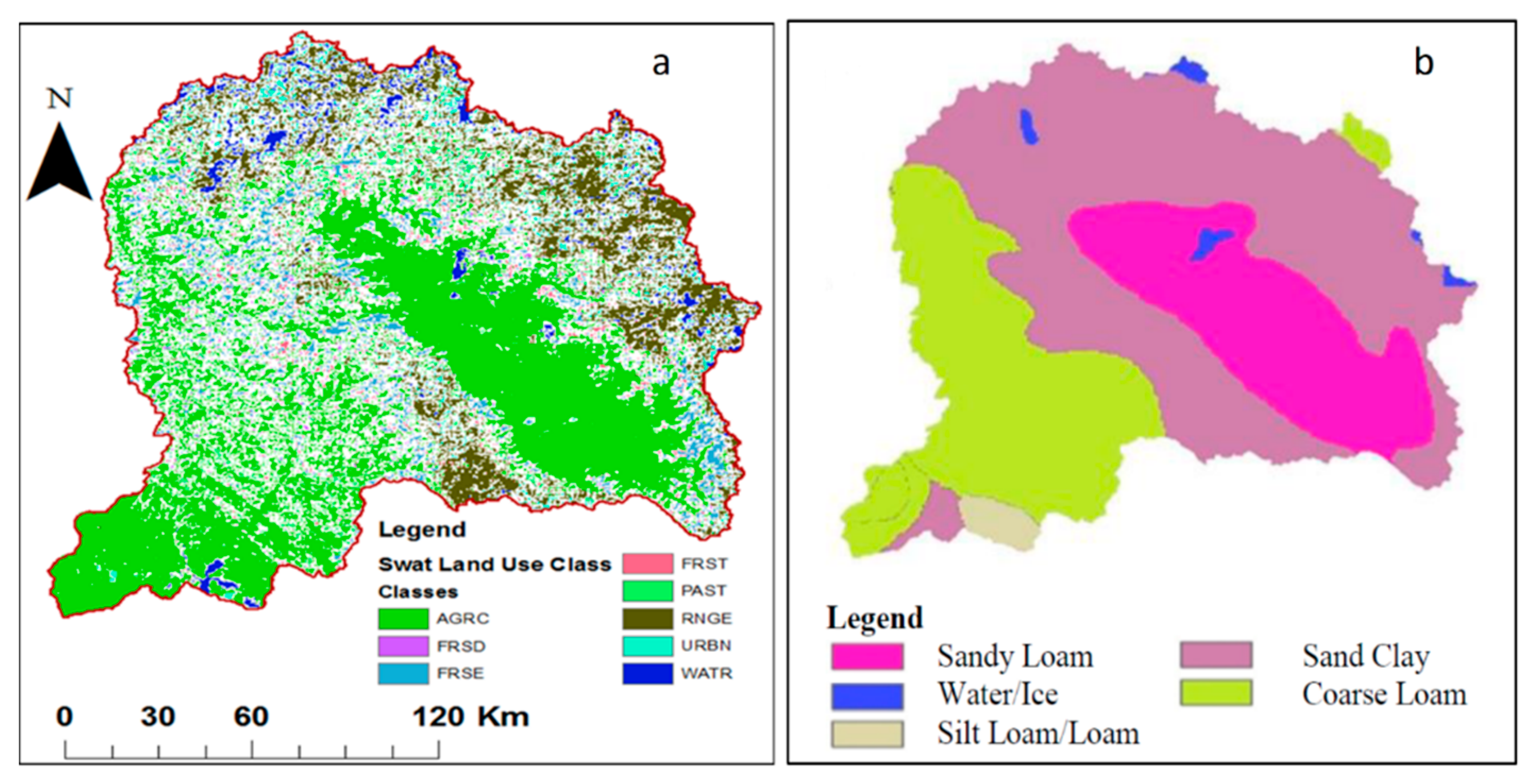
Water 12 03254 g001
Figure 2. Landuse (a) and soil (b) classes in Mangla basin.
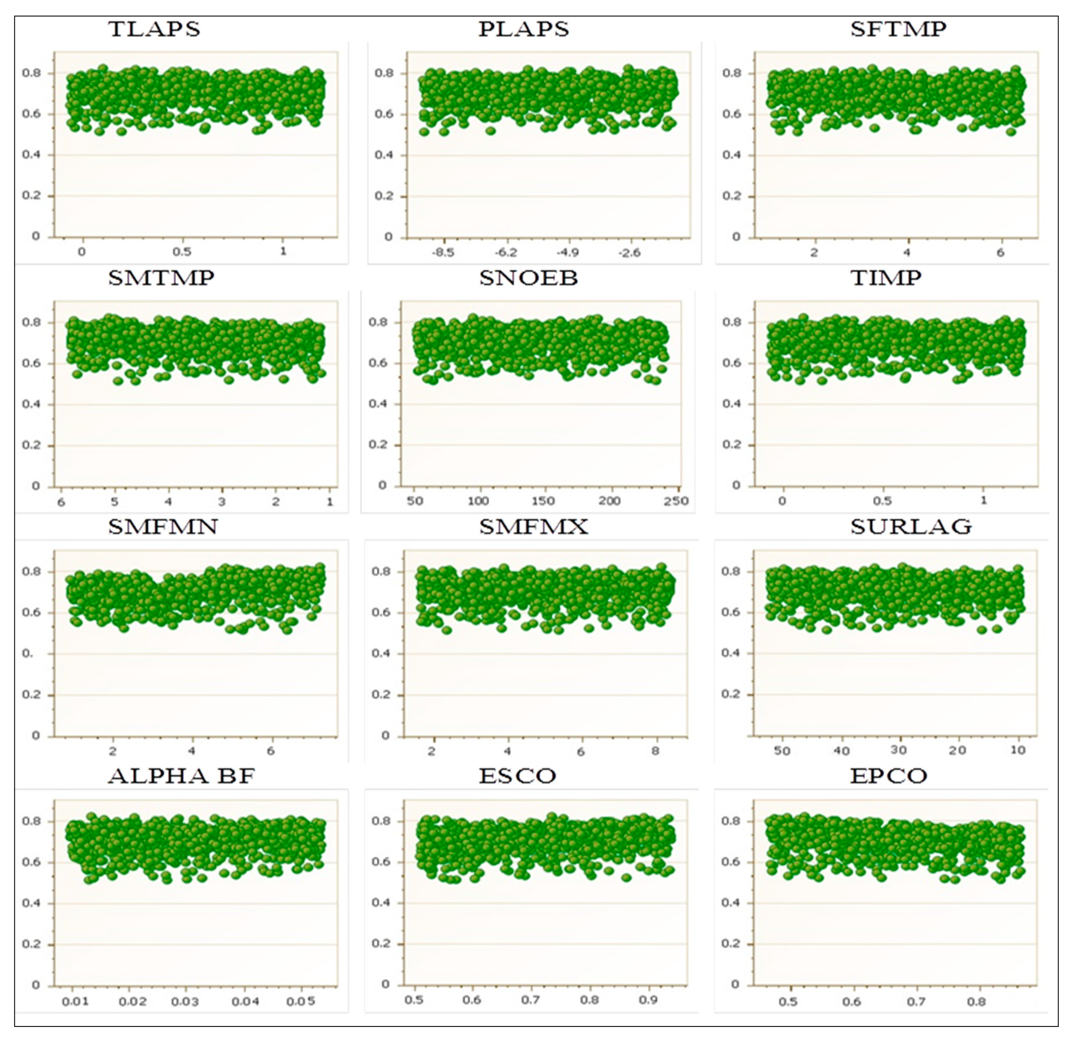
Water 12 03254 g002
Figure 3. Dotty spots exhibit the parameters variability of Soil and Water Assessment Tool (SWAT) during calibration; x-axis shows values of parameters, while y-axis represents R2 values (upper pan represents 1st calibration period 1996–2000, while, lower pan shows 2nd calibration period 2006–2010). TLAPS (Temperature lapse rate); PLAPS (Precipitation lapse rate); SFTMP (Snowfall temperature); SMTMP (Snow melt base temperature); SNOEB (Initial snow water content in elevation band); TIMP (Snow pack temperature lag factor); SMFMN (Melt factor for snow); SMFMX (Melt factor for snow); SURLAG (Surface runoff lag time); ALPHA BF (Base flow alpha factor); SOL AWC (Available water capacity); ESCO (Soil evaporation compensation factor); EPCO (Plant uptake compensation factor).
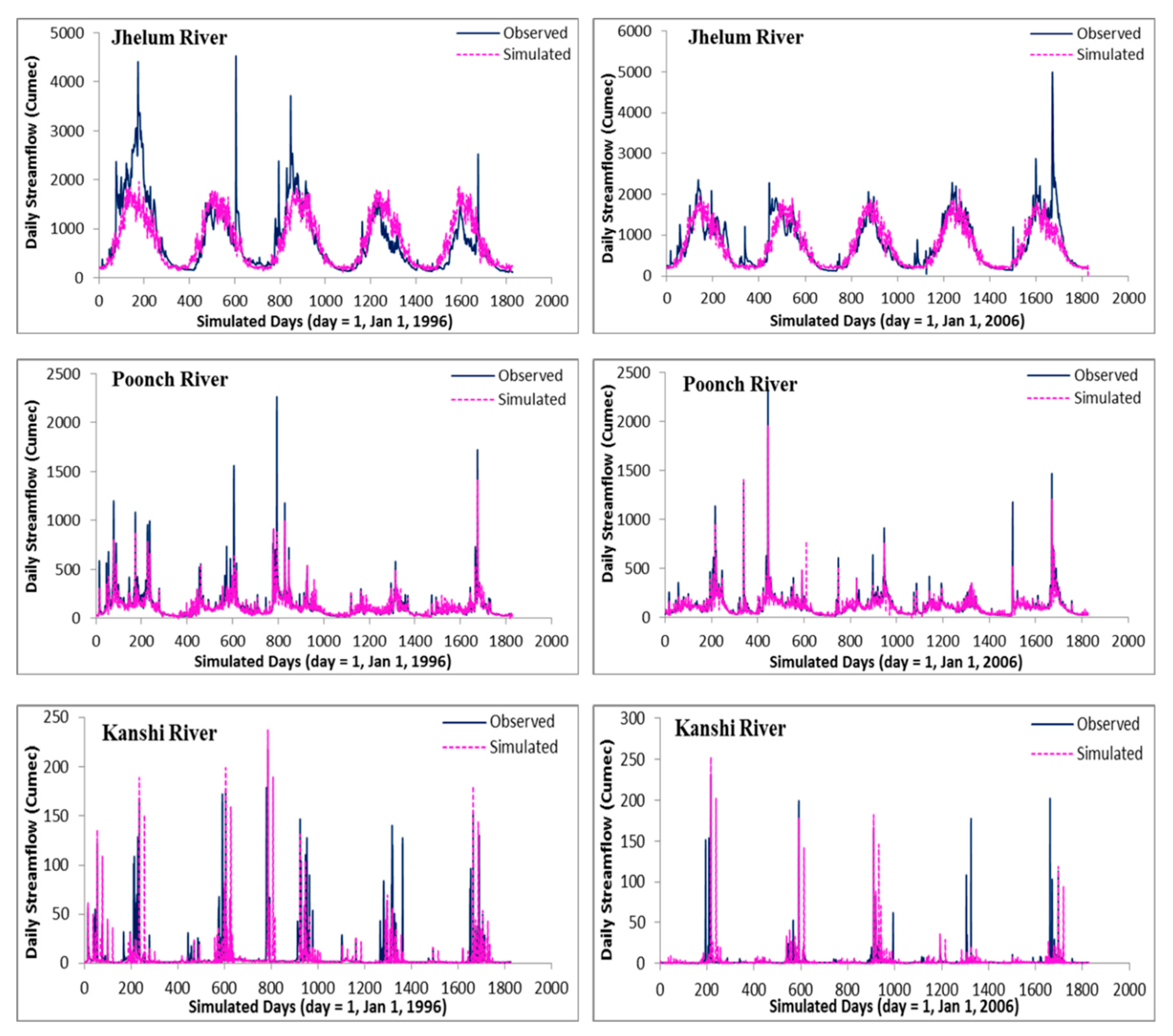
Water 12 03254 g003
Figure 4. Comparison of observed and simulated daily streamflow in all rivers of Mangla watershed for the calibration periods (left pan is for 1st calibration period 1996–2000, and right pan is for 2nd calibration period 2006–2010).
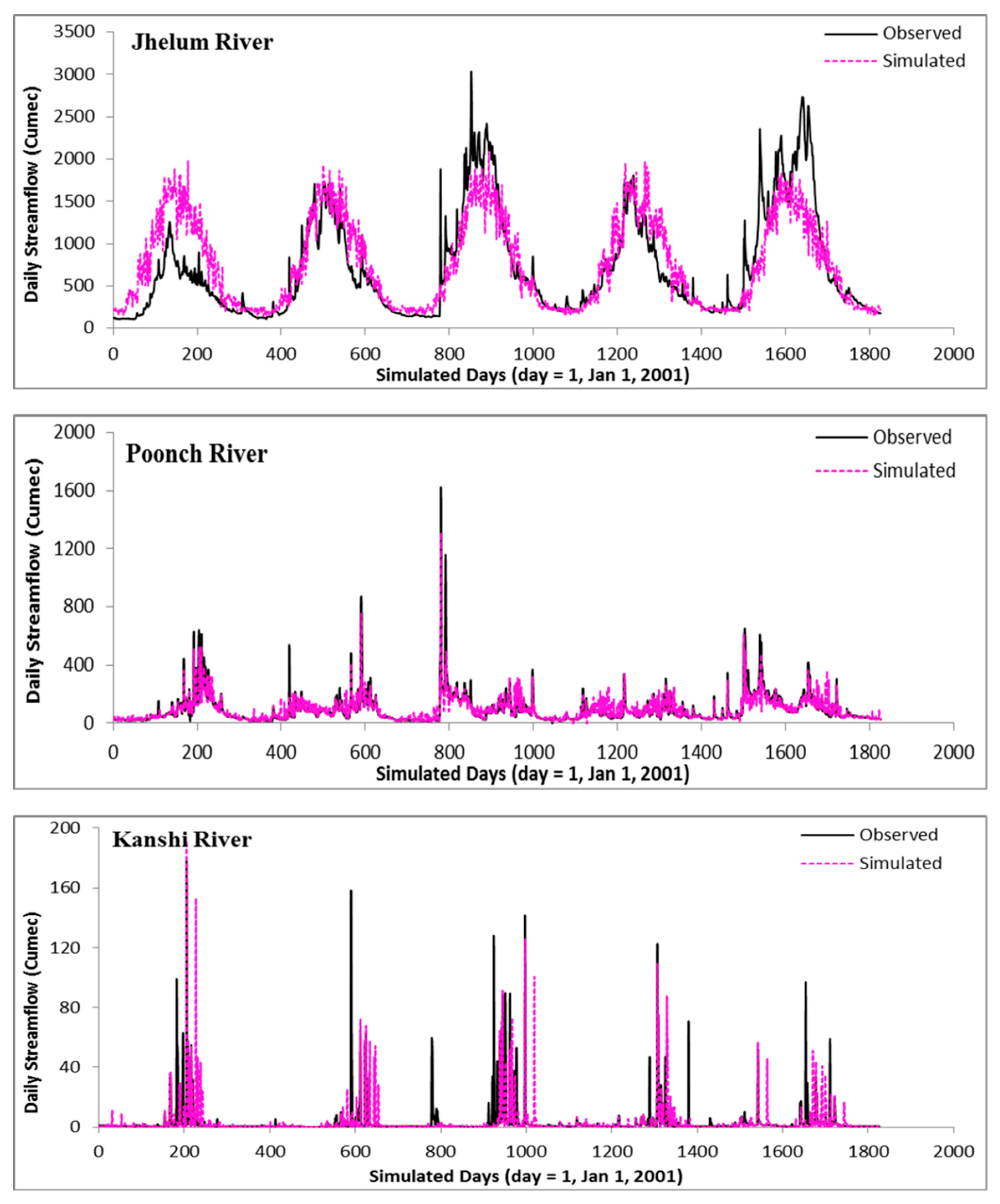
Water 12 03254 g004
Figure 5. Comparison of observed and simulated daily streamflow in all rivers of Mangla watershed for the validation period 2001–2005.
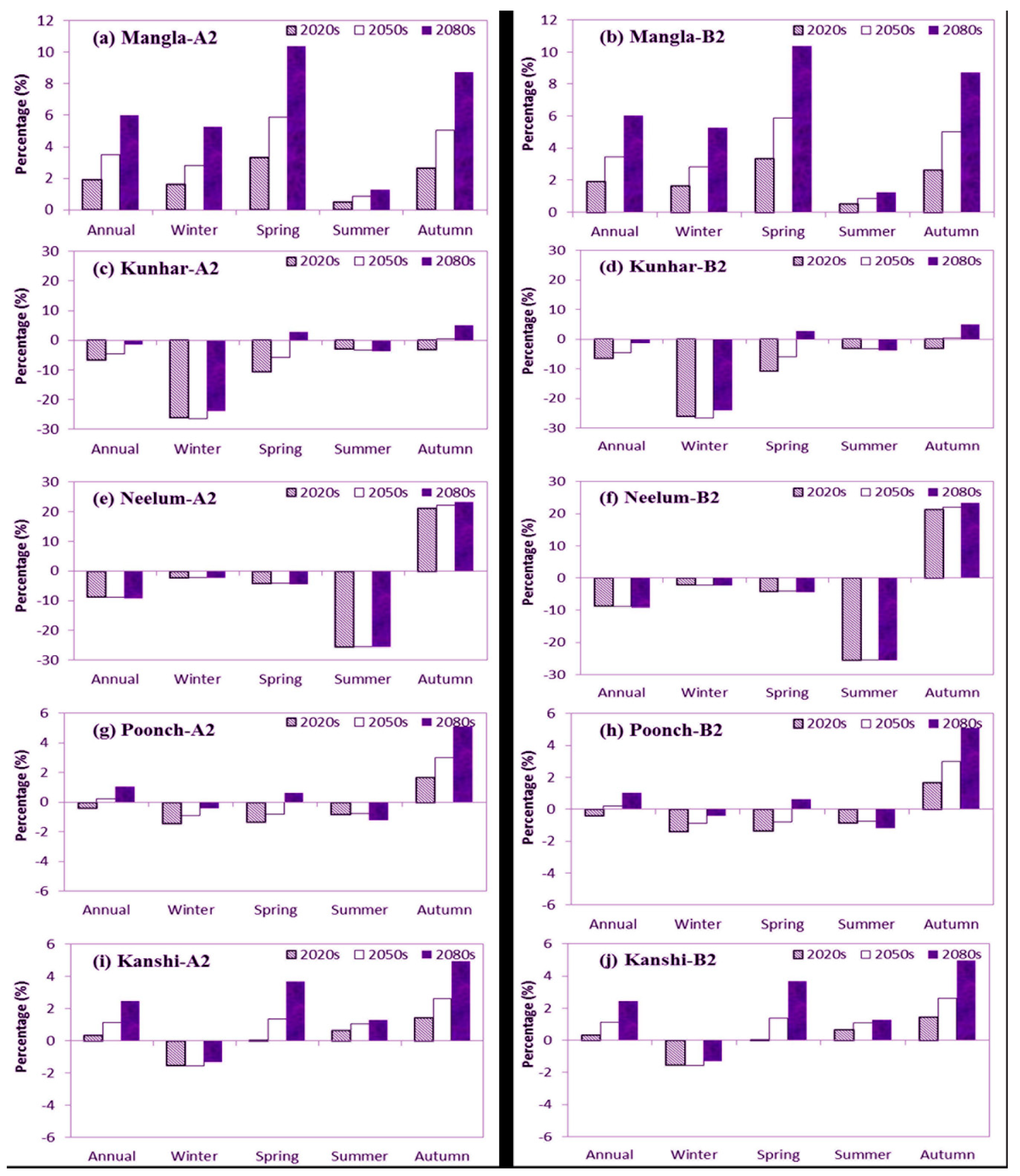
Water 12 03254 g005
Figure 6. The percentage change representing (scenarios-historical period) of seasonal and annual maximum temperature (compared to base period) in 2020s, 2050s and 2080s under A2 and B2 scenarios ((a,b) Mangla basin; (c,d) Kunhar basin; (e,f) Neelum basin, (g,h) Poonch basin and (i,j) Kanshi basin).
Water 12 03254 g006
Figure 7. The percentage change representing (scenarios-historical period) of seasonal and annual minimum temperature (compared to base period) in 2020s, 2050s and 2080s under A2 and B2 scenarios ((a,b) Mangla basin, (c,d) Kunhar basin, (e,f) Neelum basin, (g,h) Poonch basin and (i,j) Kanshi basin).
Water 12 03254 g007
Figure 8. The percentage change representing (scenarios-historical period) of seasonal and annual precipitation (compared to base period) in 2020s, 2050s and 2080s under A2 and B2 scenarios ((a,b) Mangla basin, (c,d) Kunhar basin, (e,f) Neelum basin, (g,h) Poonch basin and (i,j) Kanshi basin).
Water 12 03254 g008
Figure 9. The change percentage of monthly stream flows (compared to base period) in 2020s, 2050s and 2080s under scenarios A2 and B2 ((a,b) Jhelum River, (c,d) Poonch River, (e,f) Kanshi River and (g,h) Mangle Reservoir).
Water 12 03254 g009
Figure 10. The change percentage of annual and seasonal stream flows (compared to base period) in 2020s, 2050s and 2080s under scenarios A2 and B2 ((a,b) Jhelum River, (c,d) Poonch River, (e,f) Kanshi River and (g,h) Mangle Reservoir).
Water 12 03254 g010
Table 1. Type of data used in the present study and their source.
Data TypeSourceSpatial/Temporal ResolutionDescription/Period of Record
TopographyUSGS National Elevation Dataset90 × 90 mDEM (Elevation)
Land use dataEuropean Space Agency (ESA) Global Land Cover http://ionia1.esrin.esa.int/300 × 300 mClassified land use such as forest, agriculture, crops, water, etc.
Soil dataFAO–International Soil Reference and Information Centre (ISRIC)1 kmClassified soil and physical properties as sand, silt clay bulk density, etc.
Climate dataPakistan Meteorological Department (PMD), Water and Power Development Authority (WAPDA)DailyPrecipitation, Temperature, solar radiation, wind speed (1961–2010)
Hydrological dataWater and Power Development Authority (WAPDA)DailyStream flows (1961–2010)
Climate Scenario Data (GCM-Had CM3)Canadian Climate Scenarios Network (http://www.cics.uvic.ca/scenarios/sdsm/select.cgi)2.5° latitude 3.75° longitude Daily1961–2099
Table 2. Climatic stations in Mangla watershed.
Sr. No.StationLat (degree)Lon (degree)Elevation (m)CatchmentMax. Temp (°C)Min. Temp (°C)Precipitation (mm)
1Murree33.973.42206Jhelum17.38.91782
2Bagh34.073.81067Jhelum25.112.01482
3Mangla33.173.6282Jhelum29.717.1867
4Gujar Khan33.373.3457Kanshi28.514.9825
5Kallar33.473.4518Kanshi28.516.4973
6Balakot34.673.4995.5Kunhar25.112.21623
7Naran34.973.72363Kunhar12.02.51793
8Astore35.274.52168Neelum15.74.1488
9Garidopatta34.273.6813.5Neelum26.012.51413
10Muzaffarabad34.473.5702Neelum27.713.61484
11Kotli33.573.9610Poonch28.415.31219
12Palandri33.773.71402Poonch22.912.11390
13Rawalakot34.074.01677Poonch20.69.21369
14Khandar33.574.11067Poonch--1062
15Sehr kakota33.774.01125Poonch--1342
Table 3. Stream gauges installed in Mangla watershed.
Sr. No.StationLatitude (degree)Longitude (degree)Elevation (m)Basin Area (Km2)River NameMean Annual (Cumec m3/s)
1Naran34.973.724001107Kunhar46
2G-Habibullah34.473.48202433Kunhar102
3Muzaffarabad34.473.56707412Neelum325
4Chinari34.273.8107013,652Jhelum300
5Domel34.473.570114,396Jhelum328
6Kohala34.173.556024,464Jhelum776
7Azad Pattan33.773.648525,967Jhelum1239
8Palote33.273.4400867Kanshi6
9Kotli33.573.95303210Poonch128
Table 4. Selected predictor variables with their respective predictand.
StationPrecipitationMaximum TemperatureMinimum Temperature
Kotlishum, p5_z, p8_f, p850, rhump500, tempp500, temp, shum
Rawalakottemp, p850, mslps, p5_f, r850p500, tempp500, temp, shum
Plandrishum, p8_f, p850, p5_f, p_z, p5_up500, tempp500, temp, shum
Khandartemp, shum, p5_z, rhum, mslp, p_v, p_zh, p5_v--
Sehr Kokatatemp, shum, rhum, p5_f, p5_u--
Murreep5-z, p8-f, r850, rhum, shump500, tempp500, temp, shum
Baghp5-f, p5-u, p5th, shump500, tempp500, temp, shum
Gujar Khanmslp, p5-f, p5th, 9850, shum, tempp500, tempp500, temp, shum
Kallarmslp, p5-u, p5th, r500, shump500, tempp500, temp, shum
Manglamslp, p5th, p850 shump500, tempp500, temp, shum
Balakotp5-f, p5th, p8-f, r850, rhum, shump500, temp, shump500, temp
Muzaffarabadmslp, p5-v, p850, r850, shump500, tempp500, temp, shum
Naranp-v, p500, p5th, shum, tempp500, temp, shump500, temp, shum
Astorep-f, p-u, p-v, p8-f, rhum, tempp500, temp, shump500, temp, shum
Garidopattamslp, p-f, p-u, p-v, p8-f, rhum, tempp500, temp, shump500, temp, shum
Mslp = mean sea level pressure; rhum= near surface relative humidity; shum = surface specific humidity; p5_z = 500 hpa voritcity; p8_f = 850hpa airflow strength; r850 = relative humidity at 850 hpa; r500 = relative humidity at 500 hpa; p5-f = 850 hpa airflow strength; p5-v= 500 hp meriodinal velocity; p5th = 500 hpa wind direction; p-f = surface air flow strength; p-u = surface zonal velocity; p-v = surface meridian velocity; temp= mean temperature at 2 m.
Table 5. Comparison of determination coefficient (R2), Root Mean Square Error (RMSE), Nash-Sutcliffe Coefficient (Nr), Percent bias (PBIAS) and Mean Absolutely Error (MAE) between observed and simulated results of maximum temperature, minimum temperature and precipitation for each station in the validation period (1991–2000).
VariableR2RMSE (mm or °C/Month)NrPBIAS (%)MAE (mm or °C/Month)
RangeMeanRangeMeanRangeMeanRangeMeanRangeMean
Precipitation
NCEP0.17–0.60.3646–17293−0.1–0.60.25−11.1–29−7.832–12166
H3A20.17–0.40.2747–171105−0.8–0.30.25−10.8–26−4.733–12577
H3B20.11–0.50.2846–167103−0.6–0.30.15−10.4–14−1032–12072
Max. Temperature
NCEP0.88–0.970.931.5–3.42.20.7–10.92−11–3.5−2.41.2–2.81.7
H3A20.87–0.960.921.7–3.92.30.7–10.9312–3.9−1.41.3–3.21.7
H3B20.87–0.950.911.7–3.72.40.7–10.8911–4.2−0.71.3–31.8
Min. Temperature
NCEP0.90–.980.950.9–2.60.920.86–0.980.9240–14−2.10.7–2.11.4
H3A20.92–0.970.941.2–2.81.90.86–0.970.9318–8−0.11–2.21.5
H3B20.92–0.960.941.4–2.920.87–0.960.9215.3–9.111.1–2.31.5
Table 6. Model calibration and verification statistics for daily and monthly stream flow comparison.
Objective FunctionRivers
JhelumPoonchKanshi
Cal-P1Cal-P2ValCal-P1Cal-P2ValCal-P1Cal-P2Val
Daily Simulation
R20.8360.8190.7520.8830.8100.7100.8040.8260.697
NSE0.830.790.620.8370.770.680.850.810.74
PBIAS3.84.67.39.1−2.15.87.24.5−8.2
Monthly Simulation
R20.8930.8710.8260.9290.9410.9020.9630.8930.894
NSE0.690.8230.7290.8570.8710.930.950.890.786
PBIAS−0.935.07−5.610.120.057.465.543.645.13
Cal-P1 = Calibration Period 1st (1996–2010), Cal-P2 = Calibration Period 2nd (2006–2010). Val = Validation for the period (2001–2005).
Table 7. List of calibrated parameters and their optimized value.
ParameterDescriptionRangeOptimized Value of Parameters for Rivers
JhelumPoonchKanshi
Cal-P1Cal-P2AverageCal-P1Cal-P2AverageCal-P1Cal-P2Average
TLAPSTemperature lapse rate (°C/km)0−10−3.1−4.6−3.85−5.7−6−5.85−7−6.3−6.65
PLAPSPrecipitation lapse rate (mm H2O/km)0,10013171591110898.5
SFTMPSnowfall temperature (°C)−5 + 5333211.5
SMTMPSnow melt base temperature (°C)−5 + 52.11.71.93.13.53.3
SNOEBInitial snow water content in elevation band (mm)0,300200190195150150150
TIMPSnow pack temperature lag factor0.01,1111111
SMFMNMelt factor for snow (mm H2O/°C-day)0,10343.54.54.54.5
SMFMXMelt factor for snow (mm H2O/°C-day)0,104.244.155.35.15
SURLAGSurface runoff lag time (hrs)0,9631.328.529.917.215.816.597.88.4
CN2Runoff Curve Number54–85677068.5697069.5656565
SOL KSaturated hydraulic conductivity0.0 to 2000 0 0
ALPHA BFBase flow alpha factor0.00 to 1.000.01430.0140.014150.0120.0120.0120.0140.0140.014
SOL AWCAvailable water capacity0.0 to 1.00 0 0
ESCOSoil evaporation compensation factor0.7–1.00.950.80.8750.850.850.850.70.80.75
EPCOPlant uptake compensation factor0.4–0.90.70.70.70.70.70.7
Publisher’s Note: MDPI stays neutral with regard to jurisdictional claims in published maps and institutional affiliations.

