Assessment of Population Exposure to Urban Flood at the Building Scale


1
School of Geographic and Biologic Information, Nanjing University of Posts and Telecommunications, Nanjing 210023, China
2
Department of Civil Engineering, University of Bristol, Bristol BS8 1TR, UK
3
Key Laboratory of VGE of Ministry of Education, Nanjing Normal University, Nanjing 210023, China
*
Author to whom correspondence should be addressed.
Water 2020, 12(11), 3253; https://doi.org/10.3390/w12113253
Submission received: 30 September 2020
/
Revised: 11 November 2020
/
Accepted: 18 November 2020
/
Published: 20 November 2020
(This article belongs to the Special Issue GIS Application: Flood Risk Management)
Abstract
:The assessment of populations affected by urban flooding is crucial for flood prevention and mitigation but is highly influenced by the accuracy of population datasets. The population distribution is related to buildings during the urban floods, so assessing the population at the building scale is more rational for the urban floods, which is possible due to the abundance of multi-source data and advances in GIS technology. Therefore, this study assesses the populations affected by urban floods through population mapping at the building scale using highly correlated point of interest (POI) data. The population distribution is first mapped by downscaling the grid-based WorldPop population data to the building scale. Then, the population affected by urban floods is estimated by superimposing the population data sets onto flood areas, with flooding simulated by the LISFLOOD-FP hydrodynamic model. Finally, the proposed method is applied to Lishui City in southeast China. The results show that the population affected by urban floods is significantly reduced for different rainstorm scenarios when using the building-scale population instead of WorldPop. In certain areas, populations not captured by WorldPop can be identified using the building-scale population. This study provides a new method for estimating populations affected by urban flooding.
1. Introduction
The frequency and intensity of flooding are increasing due to climate change [1,2]. According to data from EM-DAT, floods accounted for 49% of global disasters and 68% of the affected population in 2019 [3]. Urbanization has increased the risk of urban flooding by changing topography and geological conditions, both of which influence hydrological processes [4,5]. Therefore, floods have become the main natural disaster in many cities, which are characterized by a large population and rapid urbanization, posing serious threats to human life, production, and social and economic activities [6]. As such, accurate flood risk assessments for cities are vital for formulating local disaster prevention policies.
Population is the most important flood-hit object; thus, accurate population-based spatial distribution information is an important basis for disaster prevention and mitigation [7]. The population affected by urban floods is typically calculated by superimposing population data sets on flood information. Therefore, population mapping is key for disaster assessment calculation, with higher-resolution population datasets more accurately estimating the size and spatial distribution of affected populations [8], which greatly improves the rationality of flood-related decision-making [9]. Common population datasets include census data provided by the government, with administrative divisions as statistical units; however, census data have a long update cycle and suffer from the modifiable areal unit problem (MAUP) when calculations are based on GIS [10,11]. In addition, census data based on administrative units ignore the spatial heterogeneity of population distributions, resulting in an inaccurate risk assessment. Therefore, it is difficult for traditional census data to mine microscopic dynamic laws, discover new phenomena [12], or meet the increasing requirements for accurate urban computing. To solve this problem, dynamic mapping is applied to demographic data spatialization [13], which maps demographic data according to the unit of the administrative region to a geographic grid of a certain size. Common methods include the average distribution method, spatial interpolation method, population distribution model, correlation analysis method, and remote sensing estimation. Population distribution data based on a spatial grid correlate statistical data with their spatial location, with high-resolution grids better reflecting the spatial distribution characteristics of the population [11]. After years of development, some global population distribution grid datasets have been developed, including the Gridded Population of the World (GPW), the Global Rural and Urban Mapping Project (GRUMP), LandScan, and WorldPop [14,15,16,17], with some countries or regions boasting population distribution grids with resolutions of higher than 100 m. Furthermore, various types of population distribution grid datasets have been used in disaster risk analysis and management, which has provided effective support for emergency government responses and disaster reduction and preparedness [7,9,18,19,20].
In contrast to large-scale population spatialization studies, urban population distributions are significantly related to urban infrastructure such as educational resources and transportation [21]. Urban surface conditions can be characterized by multi-source geographic data, such as social media data, volunteered geographic information, vehicle trajectory, and mobile phone data [20,22], which provide a foundation for obtaining more refined urban population data [23,24]. Some studies have suggested that buildings are a more suitable scale for high-resolution simulations of population distribution [25,26]. For example, Bakillah constructed a population distribution map at the building scale in Hamburg, Germany [27] and Yao integrated multi-source spatial data such as points of interest (POIs) and real-time Tencent user densities (RTUD) to construct a refined population distribution at the building scale in Shenzhen, China [21]. Thus, populations can be estimated at the building scale using multi-source geodata such as POI to determine the relationship between buildings and populations.
Building evaluation represents a fine-scale spatial analytics method of urban flood risk assessment [19,28]. Moreover, the spatialization of population data provided by building maps is highly suitable for urban flooding disaster assessments, as they effectively combine population and buildings. With the aim of more accurately assessing the population affected by urban floods, this study employs the population redistribution method based on the grid dataset. Lishui City in Zhejiang Province, China, is used as the study area, where the population affected by urban flooding is estimated using the building-scale population distribution map, with flooding simulated by the LISFLOOD-FP hydrodynamic model.
2. Study Area and Data
2.1. Study Area
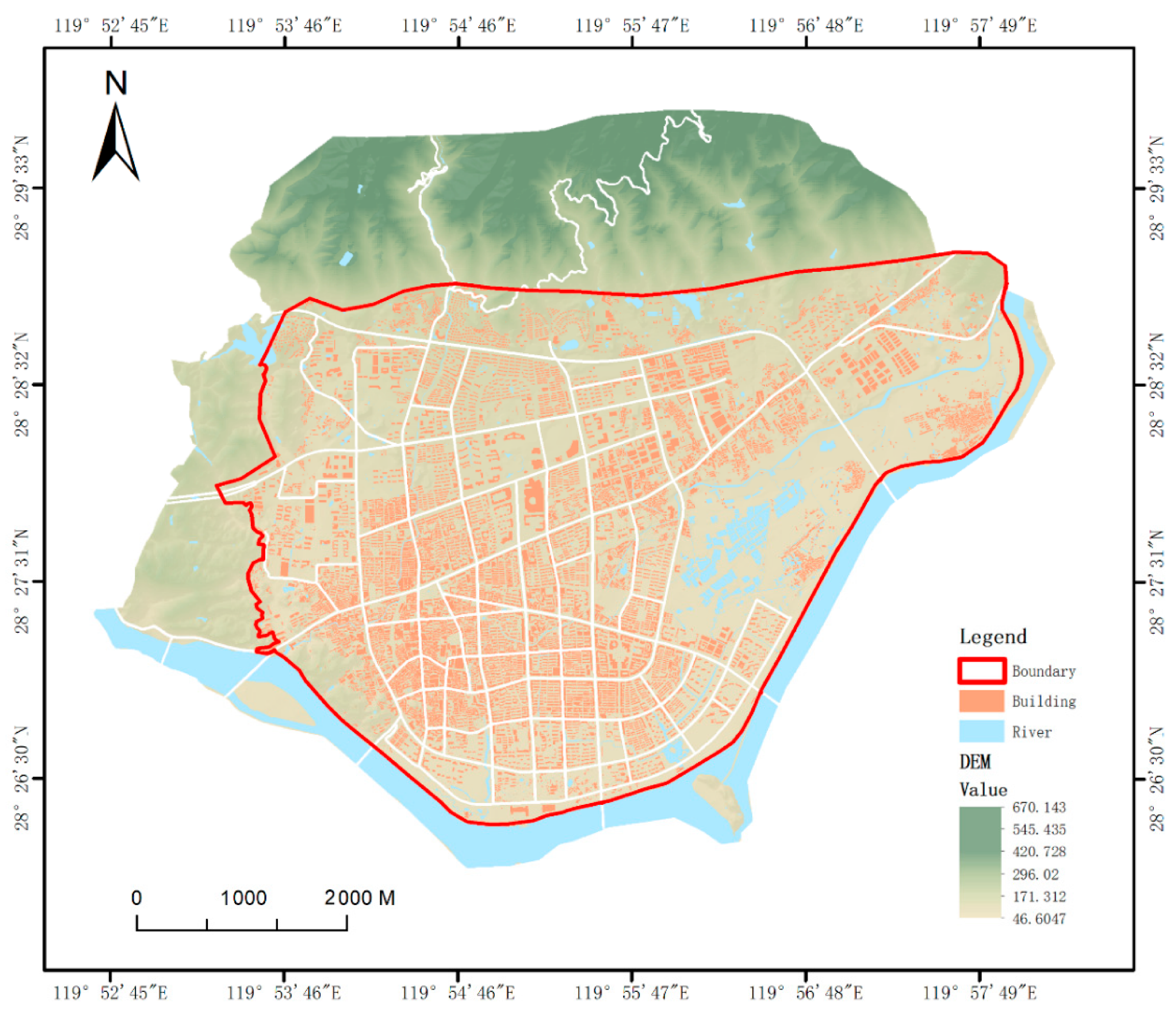
Lishui City, in Zhejiang Province, China, was selected as the experimental area for this study. This area represents the city center of Lishui, covering an area of 43.39 km in the valley of the middle reaches of the Oujiang River. The terrain is high in the north and low in the south (Figure 1). The area exhibits a subtropical monsoon climate, with a rainy season from May to October and frequent summer typhoons accompanied by local rainstorms. Flooding due to heavy rain represents a long-term disaster risk for the region; thus, high-precision assessments of the population affected by heavy rainfall has an important role in local disaster prevention and relief work.
2.2. Data Source
To solve the problem of population spatialization at the building scale and flood simulations under different scenarios, 2015 basic geographic information data, POIs, WorldPop population grid data, and census statistics for Lishui City were selected in this study.
- (1)
- Basic geographic data were provided by the Lishui City Surveying and Mapping Center, including digital elevation model (DEM), water system, transportation, building, administrative division, and underground drainage pipe network datasets. DEM data with 5 m resolution were used for terrain analysis. Administrative area and building pattern data assisted in the spatialization of demographic data. Water system and underground pipeline data were used for flood simulations.
- (2)
- POIs were obtained through the API of Baidu Maps, which is one of the most popular electronic maps in China. The total number of POIs in the study area was 11,092. To facilitate data processing, POIs were divided into 10 types including medical facilities, market shopping, restaurants, government agencies, companies, life services, education and training, residential quarters, transportation facilities, and tourist attractions.
- (3)
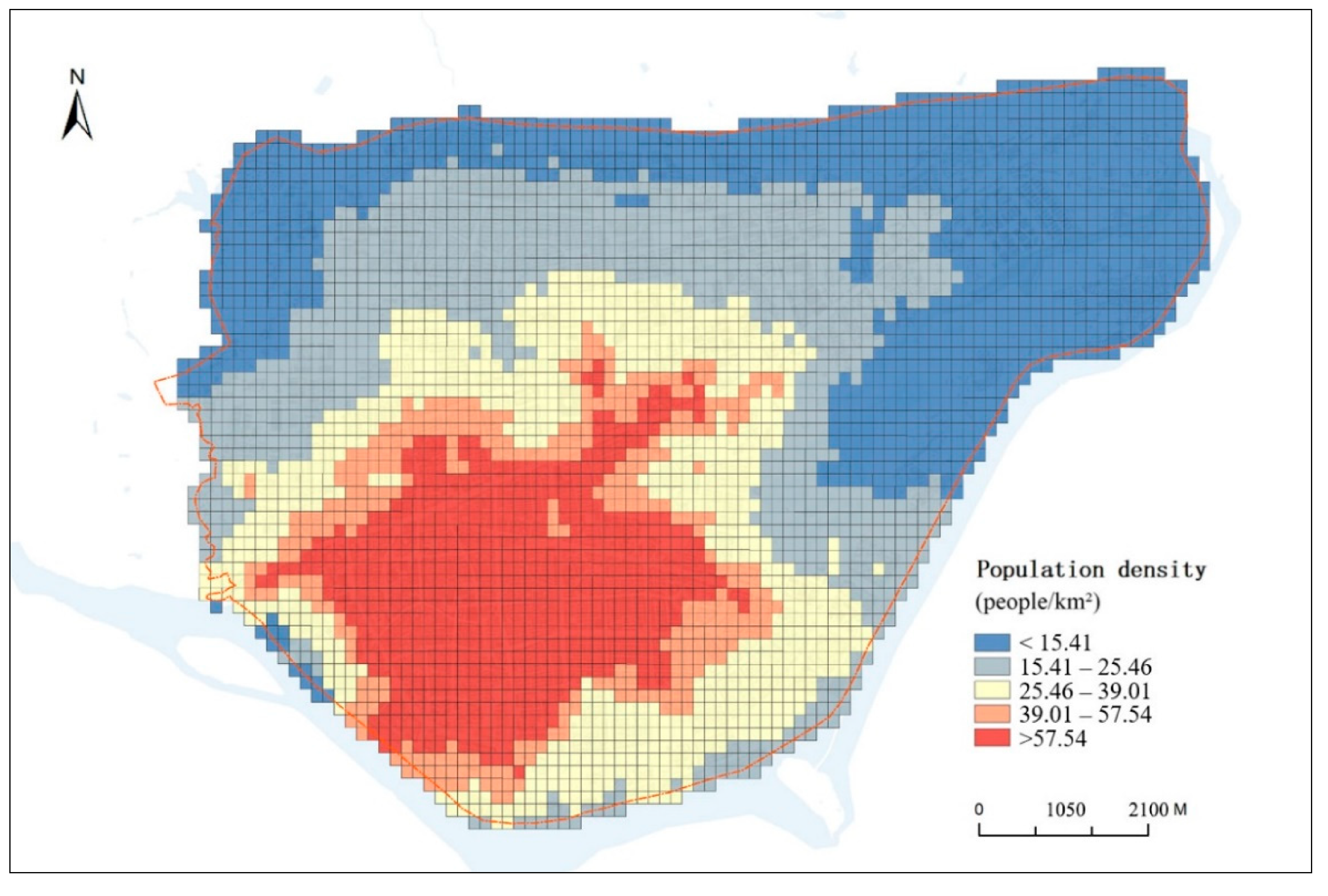
- The WorldPop dataset (the spatial distribution of population in 2015, China) was selected as the population grid dataset, which is available online (https://www.worldpop.org/geodata/summary?id=5279). Compared with other population grid datasets (GPW, GRUMP, and WorldPop), WorldPop has high accuracy and resolution in China [29] and is the result of a global population distribution mapping project led by the Geographic Data Institute of the University of Southampton in the United Kingdom. It is generated using a random forest algorithm by integrating multi-source data from population censuses, satellites, mobile devices, etc., with a grid resolution of 3 arc (approximately 100 m at the equator). This high spatial resolution means it is widely used in disaster assessment, socio-economics, and other fields. The WorldPop dataset for the study area is shown in Figure 2. From the official website of the Lishui government (http://sq.inlishui.com), we collected census data of 18 communities (25 communities in total). The WorldPop dataset has certain accuracy relative to the census, with an R2 value of 0.7673. However, the RMSE value is 3396.3060, which may be caused by the fact that the floating population is not included in the WorldPop data.
3. Methodology
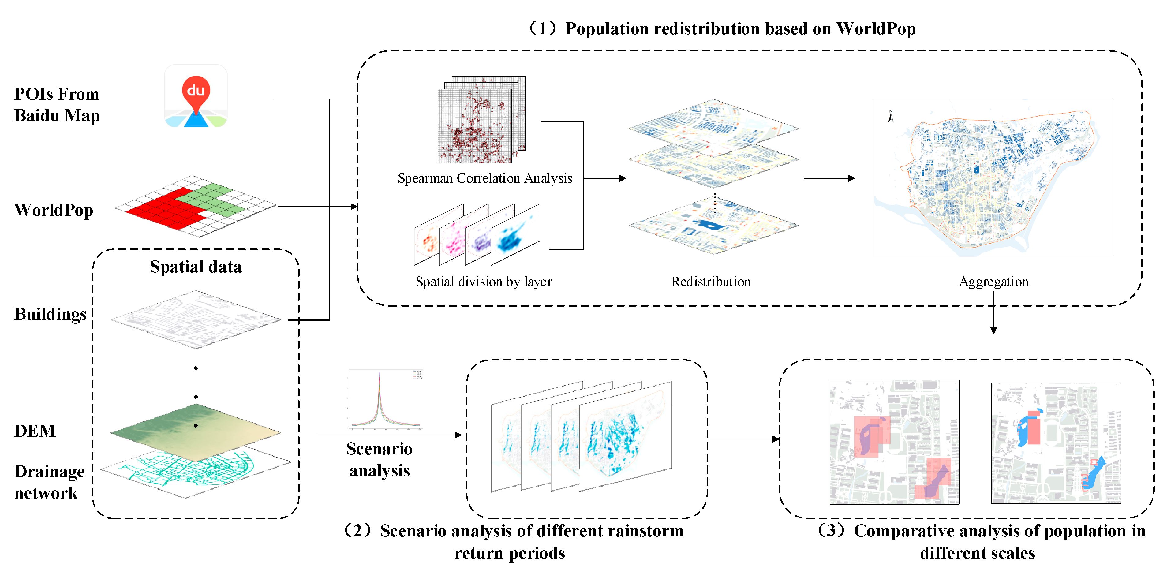
The population distribution is dynamic. However, as this study predominantly analyzed the difference between the population at the building scale and the WorldPop dataset for an urban flooding population-based risk assessment, the dynamics of the population during heavy rain disasters were ignored. First, based on the WorldPop dataset, the population grid was downscaled to the building scale by calculating the correlation coefficient between the POIs and the grid. Then, the LISFLOOD-FP model was used to simulate urban flooding under rainstorm scenarios with different return periods. Finally, the size and spatial distribution of the affected population were compared for different scenarios. The complete procedure is shown in Figure 3.
3.1. Mapping the Population at the Building Scale
To assess the flood-affected population under extreme rainfall, actual distribution data of houses and buildings were used as a constraint on the spatial distribution range of the population. The WorldPop population density grid was downscaled to the building scale, which included four main steps: (1) calculate the correlation coefficient k between the POIs of each type and the population grid, that is, assume that the total population in the study area is n and the POIs of type i represent the number of people as n*ki; (2) decompose the layers according to POI categories; (3) use Thiessen polygons to split the POI points in each type layer, and assign population data to build patches with overlay analysis; (4) synthesize all layers to obtain the total population within the building region, and evaluate the accuracy of the redistribution results.
3.1.1. Correlation Analysis between POIs and Population Grid
The correlation between population density and land-use type is often used to address the spatialization of the population. Due to the granularity of land-use functions, detailed urban uses may be neglected. For example, the land-use type of restaurants and convenience stores in residential areas is regarded as residential rather than commercial. POIs describe the location, name, and other rich semantic information of various places of concern, which represent important geographic information-based location resource data and reflect the distribution of various elements of the city [30,31,32]. POIs can indicate the distribution of the urban population and enable urban population estimation [21,24,27,33]. Using the correlation analysis method in statistics, the correlation between the population number and the number of POIs within a region can be calculated to obtain a refined population distribution. This method is simple and efficient; however, high-frequency POIs will have a greater impact on the results, for example, a road in geographic data often contains multiple POI points. When a large number of POIs belong to a certain type in a certain unit, and many small research units in the entire research area contain this type of POI, the correlation between this type of POI and the number of people will be reduced. This issue can be solved by using the term frequency-inverse document frequency (TF-IDF) algorithm [21]. According to this algorithm, if a word appears frequently in one document and rarely in others, it is considered that this word or phrase has good recognizability and is suitable for extracting the key in the document word. Similarly, if a certain type of POI appears very frequently in one area but is less numerous in another area, the functional type of this area is largely dominated by this type of POI. In our study, this approach was employed by considering population grids as the statistical unit, where the most influential type of POI for calculating the population density was that with a high frequency of occurrence in one grid but a low frequency of occurrence in other grids.
The term frequency (TF) represents the frequency of entry in the document. In this study, it represents the number of ith type in the jth grid. The calculation formula is as follows:
If the inverse document frequency (IDF) is large, this term is not significantly distinguishable. In our study, represents the total number of grids and indicates the number of grids containing the ith type.
After calculating the TF-IDF value of each type of POI, the Pearson coefficient was used to define the correlation coefficient between the ith type and population grids [21].
where is the TF-IDF value, represents the population density in the jth grid, and can be used to re-weight the population grid after normalization.
3.1.2. Population Redistribution
For each POI type, assuming that it undertakes the same functions, the closest function point should be found. Thus, the population allocated to each POI type was further allocated to each POI point. The steps are shown in Algorithm 1 and described here. First, the layers were iterated by POI type to generate Thiessen polygons for each layer, where each POI corresponds to a polygon. Then, the polygons were overlain with WorldPop layers and the population of each polygon was calculated with the population weight for that POI type. Then, the polygon and the building layer were overlain. If there was no population in the polygon, the total population without buildings was recorded and used as a correction in subsequent calculations. If a building existed within the polygon, we determined if the building was a single polygon or intersected with different polygons. If the buildings belonged to different polygons, the buildings were divided according to the boundaries of the polygon. Next, the floor area within each polygon was counted. After completing all iterations, the population of the building was calculated according to the following formula:
where POPi denotes the number of people in the ith building, is the normalization value of . and represents the weight of the jth type POI population distribution, POPij is the population of the ith building under the influence of POI type j, is the kth no-building Thiessen polygon in the layer of the jth type POI, and the distance (i,k) represents the European distance between building i and polygon k. According to the formula, the population calculation model of a building consists of two parts: initial allocation and supplementary correction. The initial allocation redistributes the Thiessen polygon formed by the gathering points of various POIs according to the proportion of the building area. Complementary corrections are then made to the population distribution based on the initial distribution in proportion to the inverse distance by the principle of geographic proximity. This ensures that the total population is not lost.
| Algorithm 1. Population Redistribution | |
| Input: POIs, Buildings B | |
| Output: | |
| 1: | For each type i |
| 2: | Create Thiessen Polygon TPi |
| 3: | Overlay TPi and Buildings B |
| 4: | For each polygon tp in TPi |
| 5: | If tp contains Building b |
| 6: | Then |
| 7: | Else |
| 8: | For each Building b |
| 9: | |
| 10: | return ; |
3.1.3. Accuracy Assessment
In population estimation research, R2 and RMSE are often used to evaluate the accuracy of the calculation results [21,27,29,34]. R2 describes the accuracy of the calculation results and RMSE is used to measure the standard error between the predicted population and the actual population. We used these two statistical indicators to evaluate the result of population redistribution by comparing the population of WorldPop grids and the population of buildings in the same block (the study area was manually divided into multiple blocks according to road network data).
3.2. Flood Model
The occurrence of urban rainstorms and flood disasters is a dynamic process, which is predominantly influenced by factors such as rainfall, surface runoff, surface confluence, and pipe network confluence. This study used the two-dimensional flood model LISFLOOD-FP model to simulate urban runoff generation and the convergence process. LISFLOOD-FP was developed by the University of Bristol in the UK and is widely used in flood simulation [35]. It is based on a grid data structure that couples one-dimensional and two-dimensional hydraulic models. LISFLOOD-FP describes the floodplain flow according to discrete continuity and momentum equations on the grid, which enables the model to represent the two-dimensional dynamic flow field of the floodplain. Since its release, it has been widely used in various research scenarios such as global river flooding and urban waterlogging, achieving good results [36,37]. The detailed parameters of the model used in this study refer to previous results from the literature [6,18] and are not described here.
3.3. Scenario Design
To simulate urban flooding disasters caused by extreme rainstorms in different scenarios, the Chicago Hyetograph Method (CHM) was used to simulate five different return periods of rainstorms (5, 10, 20, 50, and 100 years). The formula for rainstorm intensity was derived from the ‘Rainstorm Intensity Formulas of Cities in Zhejiang Province’ published by the local government.
where the variable I is the average rainstorm intensity in mm/min; the variable T is the rainfall duration (min), and P is the rainfall return period. A precipitation duration of 2 h was selected for modeling and simulation as it is considered suitable for extreme rainfall simulation in China [38]. In a certain rainfall return period, the average rainfall intensity decreases with rainfall duration. Based on this, the number of people affected by disasters at the building scale was evaluated for different scenarios then compared with the evaluation results derived using the WorldPop dataset.
4. Results and Discussion
4.1. Correlation Analysis between POIs and Population Grid
Table 1 shows that 11,092 POIs comprehensively cover 10 categories, with restaurants and hotels, market shopping, and life services accounting for the largest proportion. After overlaying the population grid and POIs, counting the number of POIs in each WorldPop grid, and calculating the TF-IDF vector of each grid, the Pearson correlation coefficient between the value and the statistical number of population grids was calculated and normalized. The results of the analysis show that the categories of market shopping, restaurants, and government institutions have a high demographic correlation, that is, a high population weighting factor, whereas the categories of tourist attractions, education and training, and transportation facilities have a lower weighting factor.
4.2. Results of Downscaling Gridded Population Mapping
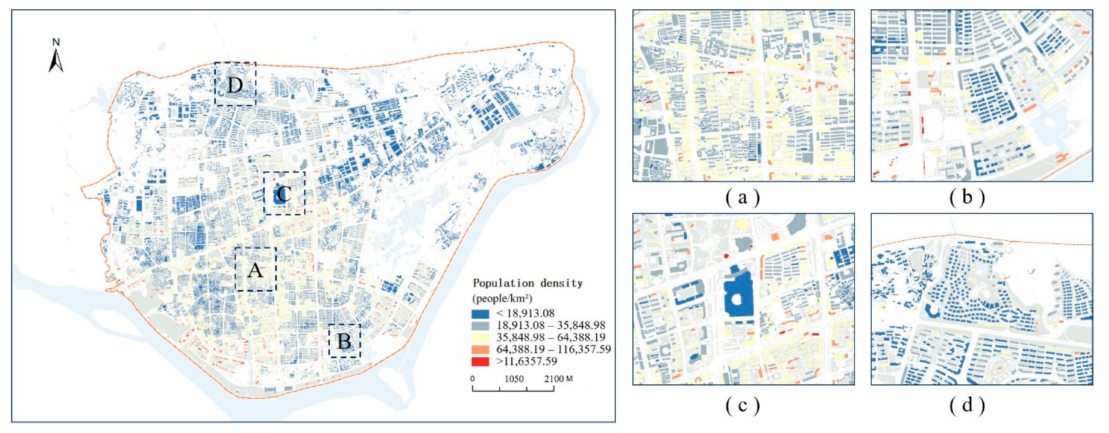
Figure 4 shows the distribution of population density at the building scale (divided into five levels by the natural breaks method). On the whole, the higher-density area overlaps with the WorldPop grid density area, revealing a trend of higher density in the center and lower density in surrounding areas, which is consistent with the characteristics of the urban population distribution model of decay with distance (WorldPop, especially prominent, as shown in Figure 2). The population distribution on the building scale shows obvious local spatial heterogeneity. In Figure 4a, the population density near the main road is higher, whereas the population density inside the block is relatively low. This is because the area near the main road is a newly built community, with relatively few surrounding POIs; thus, the population density is low (Figure 4b). Figure 4c shows that the central area is the city’s largest commercial complex, with a lower overall population density than the surrounding residential areas but a higher density of buildings. Moreover, the population density is also low at the edge of the city (Figure 4d). The above results approximately agree with the actual distribution of the residential population.
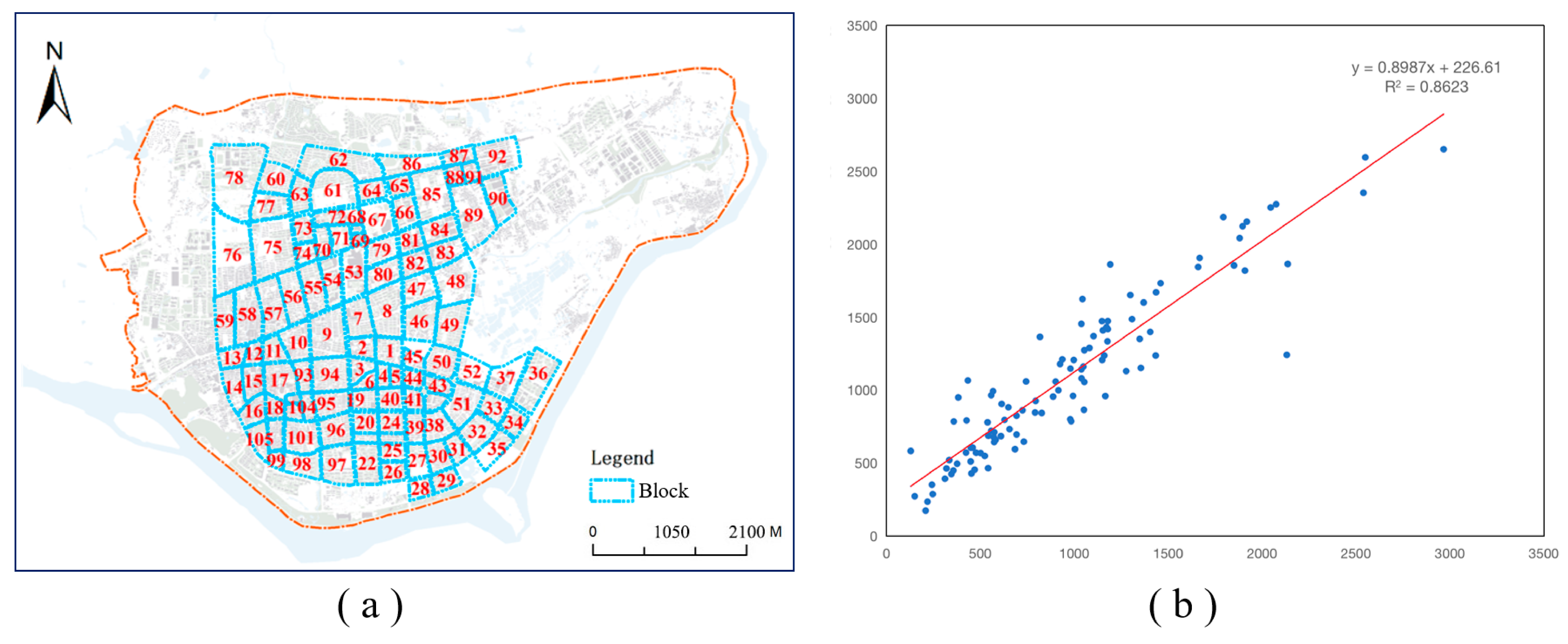
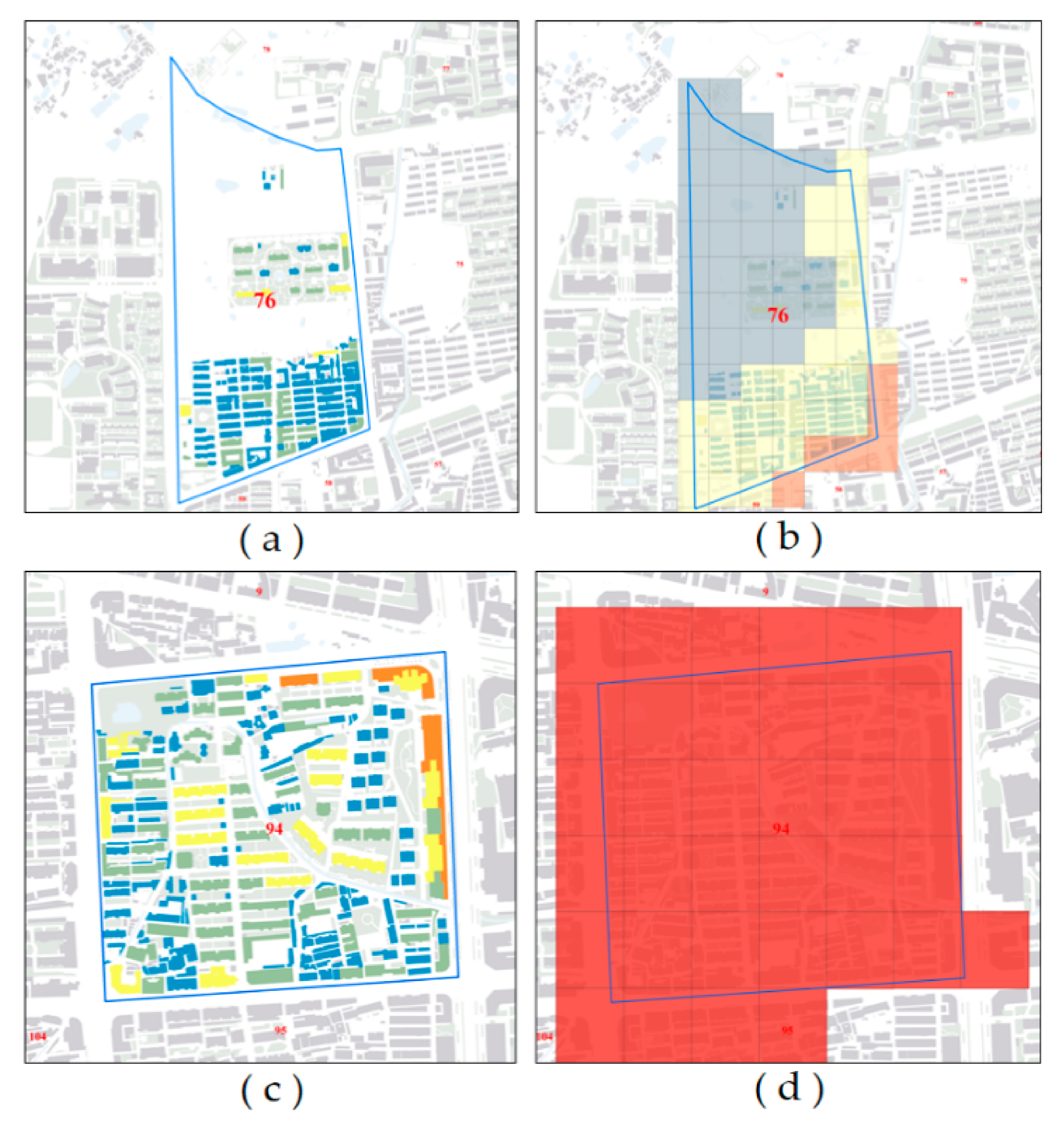
To evaluate the accuracy of the data, 105 block areas were sketched using road network data as the main reference to compare the number of people in the WorldPop grid in the block with the number of people in the building after the POI-based redistribution (Figure 5a). The R2 value between the two is 0.8623 and the RMSE value is 567.6667. The results of the regression analysis show that the building-scale population redistribution results are generally consistent with WorldPop data on a macroscopic basis (Figure 5b). Specifically, the closest is block 94, with a WorldPop population value of 1400 (after rounding) and a reassigned population assessment of 1404, representing a difference of approximately four people. The largest gap occurs in block 76, with a WorldPop population value of 951 (after rounding) and a reassigned population assessment of 382, representing a difference of approximately 569 people (Figure 6). Block 76 has fewer buildings, with an area-to-square-footage ratio of only 0.1766, whereas block 94 has more buildings and is evenly distributed, with a building-to-square-footage ratio of 0.3630. Thus, the method employed in this study has higher accuracy in urban areas where buildings are densely distributed.
4.3. Results of Flooding Simulation
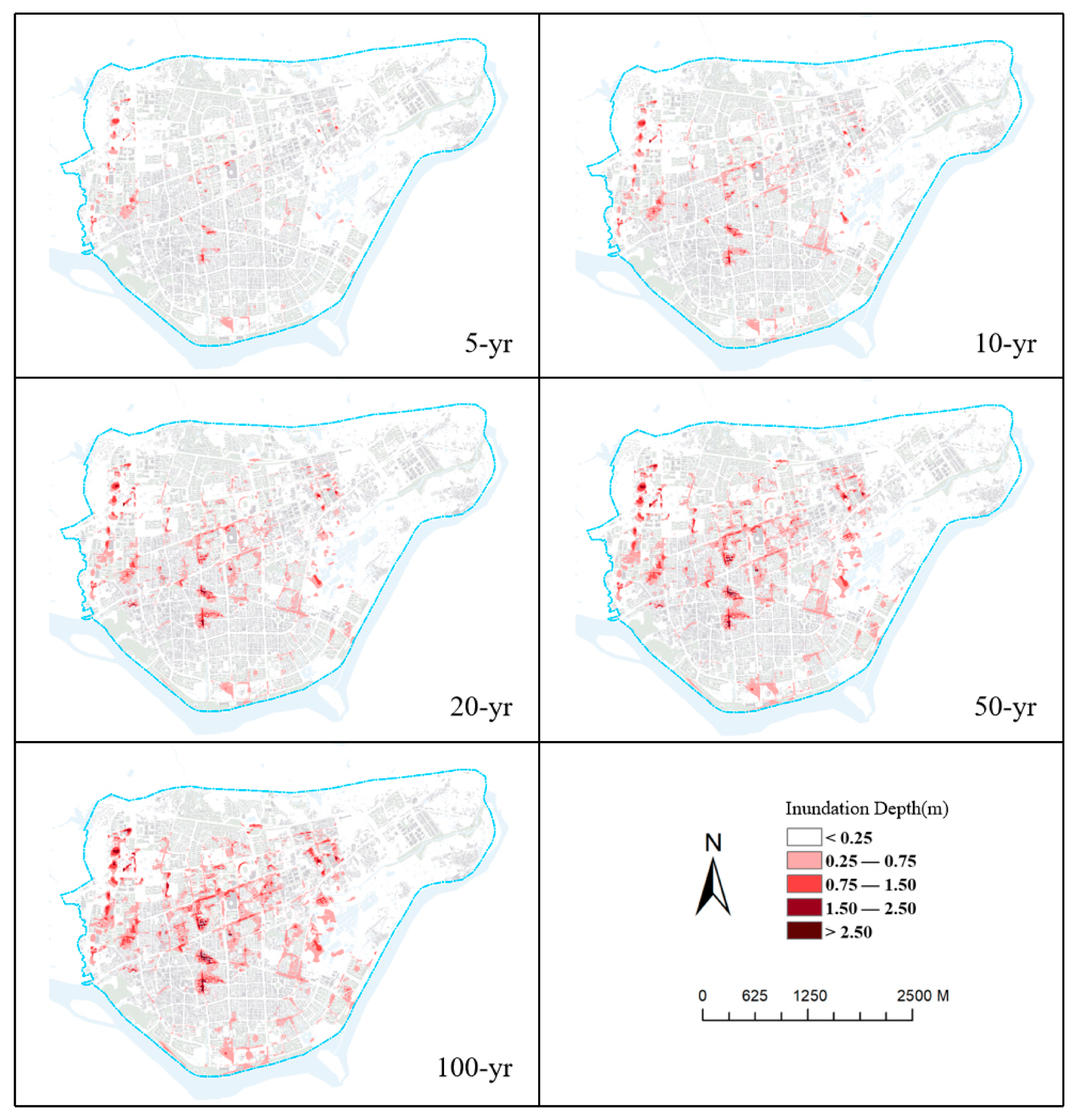
During a 2-h rainfall period, with a rain peak coefficient of 0.4, it was assumed that the rain peak would appear at approximately 48 min. The rainfall process of different rainfall return periods (5, 10, 20, 50, and 100 yr) was then calculated using the LISFLOOD-FP model. The simulation results show that different degrees of heavy rain can cause urban flooding in Lishui City (Figure 7), which is predominantly distributed along roads. When rainfall increases, the flooded area in the center of the city continues to increase. The maximum flooding depth and area are positively correlated with the rainfall return period.
As the return period of rainstorms increases, the proportion of the affected area changes significantly. The severity of urban flooding is divided into four levels according to previous literature [18]. Areas with accumulated water depths of 0.25–0.75, 0.75–1.5, 1.5–2.5 m, and greater than 2.5 m are minimally affected, moderately affected, severely affected, and critically affected, respectively. As the return period of rainstorms continues to increase, the proportion of minimally affected areas gradually decrease, whereas the proportion of severely and extremely severely affected areas gradually increases. According to the statistics of building disasters under different scenarios (Table 2), the decline in the proportion of minimally affected areas is not significant, and the proportion of moderate disasters remains relatively stable. For extremely severely affected buildings, the areal proportion also increases slightly.
4.4. Assessment of the Affected Population
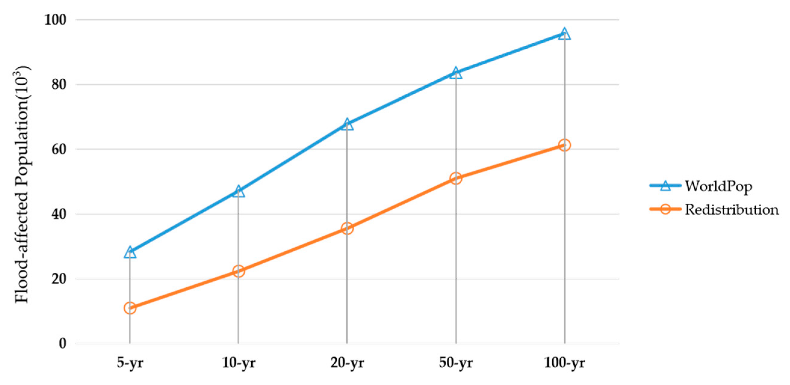
The size of the affected population can be estimated by superimposing different flood simulation results onto the population dataset. According to the results of the flood simulation, the center urban area, especially the densely populated residential area, is seriously affected. Thus, the waterlogging problem in the urban area of Lishui City is likely caused by insufficient drainage capacity in the city center. The denser the population, the greater the risk. As shown in Figure 8, rainstorms and flood disasters have a substantial impact on the population in the study area. According to the WorldPop dataset, 28,301 people are affected by rainfall with a 5-yr return period, accounting for 13.48% of the total population. Extreme rainfall with a 100-yr return period affects 95,761 people, accounting for 45.60% of the total population. A comparison with the population dataset after redistribution shows that the total number of people affected by the disaster decreases significantly, by at least one-third under all five scenarios. Thus, the number of people affected by the disaster is overestimated by the WorldPop population grid with a resolution of 3 arc.
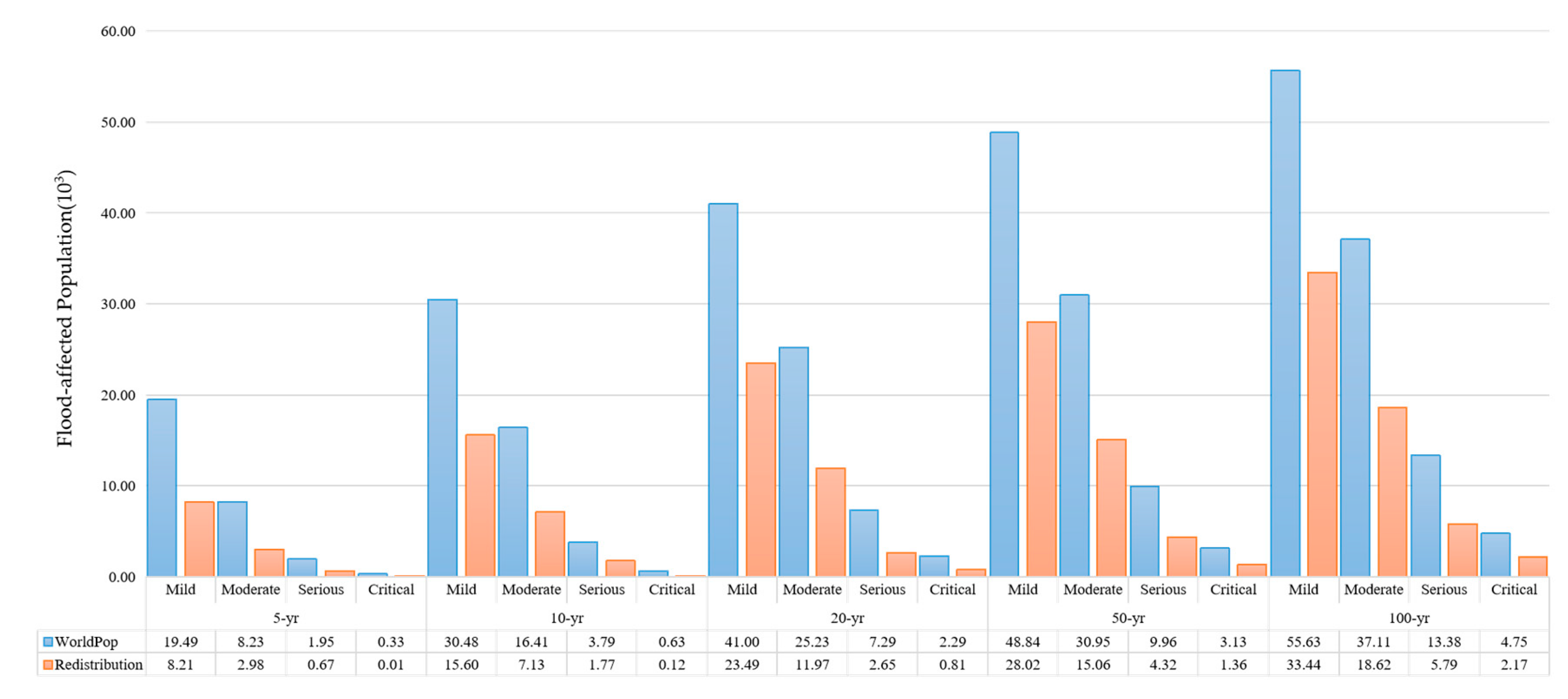
Figure 9 shows the number of people affected by different extents of urban flooding for different rainfall return periods. The assessment of the affected population at the building scale shows a decline in the number of minimally affected, moderately affected, severely affected, and critically affected. Particularly, the number of the severely and critically affected population decreased significantly. It will make the disaster assessment more targeted.
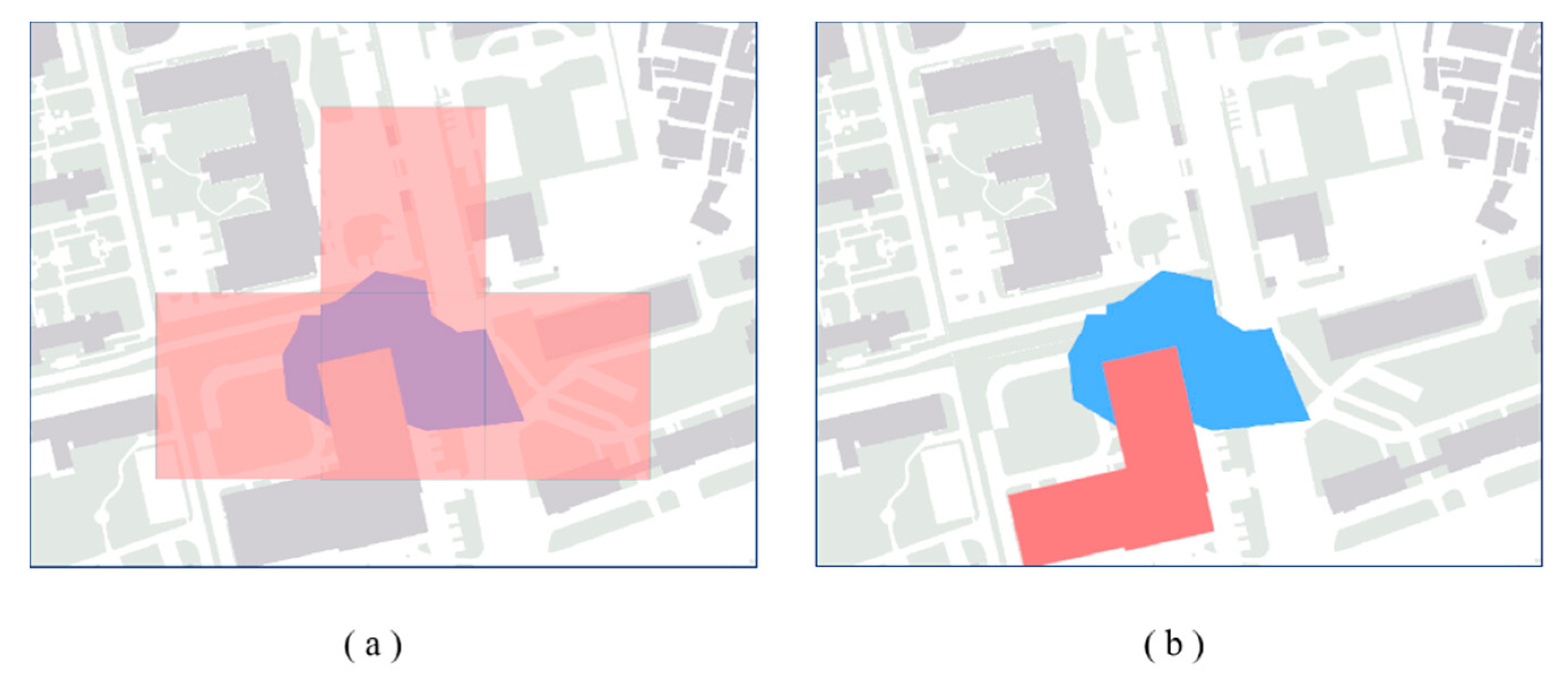
However, not all cases are overestimated when analyzing at the microscopic scale in Figure 10. When the WorldPop grid is used to evaluate the affected population, the total number of people affected by the four grids is approximately 118, whereas the affected population is 164 when the redistributed building population is used for the evaluation. Thus, although the calculated area is lower, the size of the affected population is higher. Therefore, if the WorldPop dataset is used to calculate this scenario, the disaster situation and assessment are underestimated.
5. Conclusions
Considering that the population distribution is highly related to the building distribution during urban flooding, this study assessed the population affected by urban floods using population mapping at the building scale. The building-scale population was mapped by calculating the correlation coefficient between the POI type and WorldPop population grid to establish the relationship between building function and population distribution. The urban area of Lishui City in Zhejiang Province, China, was used as the experimental area, where the affected population was estimated under different rainstorm scenarios. The results showed that the population affected by urban flooding was significantly reduced under different rainstorm scenarios when using the building-scale population instead of WorldPop. This is because the WorldPop grids of the inundated area may cover open areas such as parks and green spaces, which have a negligible population during rainstorms. Moreover, the population neglected by WorldPop could be identified by the building-scale population in some areas, especially when the building-scale population was larger than the population in the affected grids.
The aim of this study was to explore the impact of different dataset spatial scales on the assessment of flood-affected populations. The results indicate that building-scale assessments can improve the relevance and effectiveness of emergency risk management in cities. Although the WorldPop dataset was used in this study, the proposed method could be applied to other datasets to calculate the building-scale population, which would inevitably increase the accuracy of the spatialization results of the population. Furthermore, as the urban population is highly dynamic and the spatialization of demographic data is a top-down analysis method, future work should consider people’s dynamic characteristics when evaluating the population affected by urban flooding.
Author Contributions
S.Z. was responsible for literature search, setting up experiments, completing most of the experiments, and writing the original draft. B.Z. principally conceived the idea and design of the study. Q.D. modified the manuscript. J.S. processed the data and verified the experiment. All authors have read and agreed to the published version of the manuscript.
Funding
This work was supported by the National Natural Science Foundation of China (Grant Nos. 41501438, 41871299, 41771424)
Acknowledgments
We thank the National Natural Science Foundation of China (Grant Nos. 41501438, 41871299, 41771424) for providing financial support. We also thank the Lishui City Surveying and Mapping Center for providing research data.
Conflicts of Interest
The authors declare no conflict of interest.
References
- Edenhofer, O. Climate Change 2014: Mitigation of Climate Change; Cambridge University Press: Cambridge, UK, 2015; Volume 3, ISBN 1-107-05821-X. [Google Scholar]
- UNISDR. The Human Cost of Natural Disasters: A Global Perspective; Centre for Research on the Epidemiology of Disaster (CRED): Brussels, Belgium, 2015. [Google Scholar]
- CRED Crunch 58—Disaster Year in Review (2019); CRED: Brussels, Belgium, 2019.
- Hallegatte, S.; Green, C.; Nicholls, R.J.; Corfee-Morlot, J. Future flood losses in major coastal cities. Nat. Clim. Chang. 2013, 3, 802–806. [Google Scholar] [CrossRef]
- Gain, A.K.; Mojtahed, V.; Biscaro, C.; Balbi, S.; Giupponi, C. An integrated approach of flood risk assessment in the eastern part of Dhaka City. Nat. Hazards 2015, 79, 1499–1530. [Google Scholar] [CrossRef] [Green Version]
- Dai, Q.; Zhu, X.; Zhuo, L.; Han, D.; Liu, Z.; Zhang, S. A hazard-human coupled model (HazardCM) to assess city dynamic exposure to rainfall-triggered natural hazards. Environ. Model. Softw. 2020, 127, 104684. [Google Scholar] [CrossRef]
- Freire, S.; Aubrecht, C. Integrating population dynamics into mapping human exposure to seismic hazard. Nat. Hazards Earth Syst. Sci. 2012, 12, 3533–3543. [Google Scholar] [CrossRef]
- Dell’Acqua, F.; Gamba, P.; Jaiswal, K. Spatial aspects of building and population exposure data and their implications for global earthquake exposure modeling. Nat. Hazards 2013, 68, 1291–1309. [Google Scholar] [CrossRef]
- Smith, A.; Bates, P.D.; Wing, O.; Sampson, C.; Quinn, N.; Neal, J. New estimates of flood exposure in developing countries using high-resolution population data. Nat. Commun. 2019, 10. [Google Scholar] [CrossRef] [Green Version]
- Langford, M.; Higgs, G.; Radcliffe, J.; White, S. Urban population distribution models and service accessibility estimation. Comput. Environ. Urban Syst. 2008, 32, 66–80. [Google Scholar] [CrossRef]
- Wu, C.; Murray, A.T. A cokriging method for estimating population density in urban areas. Comput. Environ. Urban Syst. 2005, 29, 558–579. [Google Scholar] [CrossRef]
- Batty, M. Fifty Years of Urban Modeling: Macro-Statics to Micro-Dynamics. In The Dynamics of Complex Urban Systems; Physica-Verlag HD: Heidelberg, Germany, 2007; pp. 1–20. [Google Scholar]
- Mennis, J. Generating Surface Models of Population Using Dasymetric Mapping. Prof. Geogr. 2003, 55, 31–42. [Google Scholar] [CrossRef]
- Deichmann, U.; Street, H.; Balk, D.; Yetman, G. Transforming Population Data for Interdisciplinary Usages: From Census to Grid; Center for International Earth Science Information Network: Washington, DC, USA, 2001. [Google Scholar]
- Balk, D.L.; Deichmann, U.; Yetman, G.; Pozzi, F.; Hay, S.I.; Nelson, A. Determining Global Population Distribution: Methods, Applications and Data. In Advances in Parasitology; Elsevier: Amsterdam, The Netherlands, 2006; Volume 62, pp. 119–156. ISBN 978-0-12-031762-2. [Google Scholar]
- LandScan: A global population database for estimating populations at risk. In Remotely-Sensed Cities; Mesev, V. (Ed.) CRC Press: Boca Raton, FL, USA, 2003; pp. 301–314. ISBN 978-0-429-18116-0. [Google Scholar]
- Gaughan, A.E.; Stevens, F.R.; Linard, C.; Jia, P.; Tatem, A.J. High Resolution Population Distribution Maps for Southeast Asia in 2010 and 2015. PLoS ONE 2013, 8, e55882. [Google Scholar] [CrossRef]
- Zhu, X.; Dai, Q.; Han, D.; Zhuo, L.; Zhu, S.; Zhang, S. Modeling the high-resolution dynamic exposure to flooding in a city region. Hydrol. Earth Syst. Sci. 2019, 23, 3353–3372. [Google Scholar] [CrossRef] [Green Version]
- Hossain, M.K.; Meng, Q. A fine-scale spatial analytics of the assessment and mapping of buildings and population at different risk levels of urban flood. Land Use Policy 2020, 99, 104829. [Google Scholar] [CrossRef]
- Kounadi, O.; Ristea, A.; Leitner, M.; Langford, C. Population at risk: Using areal interpolation and Twitter messages to create population models for burglaries and robberies. Cartogr. Geogr. Inf. Sci. 2018, 45, 205–220. [Google Scholar] [CrossRef] [PubMed]
- Yao, Y.; Liu, X.; Li, X.; Zhang, J.; Liang, Z.; Mai, K.; Zhang, Y. Mapping fine-scale population distributions at the building level by integrating multisource geospatial big data. Int. J. Geogr. Inf. Sci. 2017, 1–25. [Google Scholar] [CrossRef]
- Yu, B.; Lian, T.; Huang, Y.; Yao, S.; Ye, X.; Chen, Z.; Yang, C.; Wu, J. Integration of nighttime light remote sensing images and taxi GPS tracking data for population surface enhancement. Int. J. Geogr. Inf. Sci. 2019, 33, 687–706. [Google Scholar] [CrossRef]
- Song, Y.; Huang, B.; Cai, J.; Chen, B. Dynamic assessments of population exposure to urban greenspace using multi-source big data. Sci. Total Environ. 2018, 634, 1315–1325. [Google Scholar] [CrossRef]
- Zhao; Li; Zhang; Du Improving the Accuracy of Fine-Grained Population Mapping Using Population-Sensitive POIs. Remote Sens. 2019, 11, 2502. [CrossRef] [Green Version]
- Dong, P.; Ramesh, S.; Nepali, A. Evaluation of small-area population estimation using LiDAR, Landsat TM and parcel data. Int. J. Remote Sens. 2010, 31, 5571–5586. [Google Scholar] [CrossRef]
- Silván-Cárdenas, J.L.; Wang, L.; Rogerson, P.; Wu, C.; Feng, T.; Kamphaus, B.D. Assessing fine-spatial-resolution remote sensing for small-area population estimation. Int. J. Remote Sens. 2010, 31, 5605–5634. [Google Scholar] [CrossRef]
- Bakillah, M.; Liang, S.; Mobasheri, A.; Jokar Arsanjani, J.; Zipf, A. Fine-resolution population mapping using OpenStreetMap points-of-interest. Int. J. Geogr. Inf. Sci. 2014, 28, 1940–1963. [Google Scholar] [CrossRef]
- de Ruig, L.T.; Haer, T.; de Moel, H.; Botzen, W.J.W.; Aerts, J.C.J.H. A micro-scale cost-benefit analysis of building-level flood risk adaptation measures in Los Angeles. Water Resour. Econ. 2019, 100147. [Google Scholar] [CrossRef]
- Bai, Z.; Wang, J.; Wang, M.; Gao, M.; Sun, J. Accuracy Assessment of Multi-Source Gridded Population Distribution Datasets in China. Sustainability 2018, 10, 1363. [Google Scholar] [CrossRef] [Green Version]
- Hu, S.; He, Z.; Wu, L.; Yin, L.; Xu, Y.; Cui, H. A framework for extracting urban functional regions based on multiprototype word embeddings using points-of-interest data. Comput. Environ. Urban Syst. 2020, 80, 101442. [Google Scholar] [CrossRef]
- Gao, S.; Janowicz, K.; Couclelis, H. Extracting urban functional regions from points of interest and human activities on location-based social networks. Trans. GIS 2017, 21, 446–467. [Google Scholar] [CrossRef]
- Niu, N.; Liu, X.; Jin, H.; Ye, X.; Liu, Y.; Li, X.; Chen, Y.; Li, S. Integrating multi-source big data to infer building functions. Int. J. Geogr. Inf. Sci. 2017, 31, 1871–1890. [Google Scholar] [CrossRef]
- Yang, X.; Ye, T.; Zhao, N.; Chen, Q.; Yue, W.; Qi, J.; Zeng, B.; Jia, P. Population Mapping with Multisensor Remote Sensing Images and Point-Of-Interest Data. Remote Sens. 2019, 11, 574. [Google Scholar] [CrossRef] [Green Version]
- Chen, Y.; Zhang, R.; Ge, Y.; Jin, Y.; Xia, Z. Downscaling Census Data for Gridded Population Mapping With Geographically Weighted Area-to-Point Regression Kriging. IEEE Access 2019, 7, 149132–149141. [Google Scholar] [CrossRef]
- Bates, P.D.; De Roo, A.P.J. A simple raster-based model for flood inundation simulation. J. Hydrol. 2000, 236, 54–77. [Google Scholar] [CrossRef]
- Horritt, M.S.; Bates, P.D. Evaluation of 1D and 2D numerical models for predicting river flood inundation. J. Hydrol. 2002, 268, 87–99. [Google Scholar] [CrossRef]
- Wood, M.; Hostache, R.; Neal, J.; Wagener, T.; Giustarini, L.; Chini, M.; Corato, G.; Matgen, P.; Bates, P. Calibration of channel depth and friction parameters in the LISFLOOD-FP hydraulic model using medium-resolution SAR data and identifiability techniques. Hydrol. Earth Syst. Sci. 2016, 20, 4983–4997. [Google Scholar] [CrossRef] [Green Version]
- Yang, Q.; Dai, Q.; Han, D.; Zhu, X.; Zhang, S. Impact of the storm sewer network complexity on flood simulations according to the stroke scaling method. Water 2018, 10, 645. [Google Scholar] [CrossRef] [Green Version]
Figure 1.
Map of the study area.

Figure 2.
Gridded population distribution map from WorldPop (1 November 2018).

Figure 3.
Workflow of the urban flooding population-based risk assessment at the building scale.

Figure 4.
Map of population distribution at the building scale. Map of population distribution at the building scale: (a) population distribution in block A; (b) population distribution in block B; (c) population distribution in block C; (d) population distribution in block D.
Figure 4.
Map of population distribution at the building scale. Map of population distribution at the building scale: (a) population distribution in block A; (b) population distribution in block B; (c) population distribution in block C; (d) population distribution in block D.

Figure 5.
Accuracy evaluation: (a) divided assessment unit; (b) scatterplot between WorldPop and redistribution results.
Figure 5.
Accuracy evaluation: (a) divided assessment unit; (b) scatterplot between WorldPop and redistribution results.

Figure 6.
Partial comparison of redistributed population and WorldPop estimation results: (a) population distribution at block 76 at the building scale; (b) WorldPop population distribution in block 76; (c) population distribution at the building scale in block 94; (d) WorldPop population distribution in block 94.

Figure 7.
Flooding simulation results under different rainfall return periods (5, 10, 20, 50, and 100 yr).
Figure 7.
Flooding simulation results under different rainfall return periods (5, 10, 20, 50, and 100 yr).

Figure 8.
Comparison of the number of people affected by urban flooding in multiple scenarios (5, 10, 20, 50, and 100 yr return periods).
Figure 8.
Comparison of the number of people affected by urban flooding in multiple scenarios (5, 10, 20, 50, and 100 yr return periods).

Figure 9.
Comparison of the extent of urban flooding under different rainfall return periods.

Figure 10.
Underestimation of the affected population: (a) using WorldPop grid to assess the affected population and (b) using the redistributed building population.
Figure 10.
Underestimation of the affected population: (a) using WorldPop grid to assess the affected population and (b) using the redistributed building population.


Table 1.
Correlation between POIs and the population grid.
| ID | Type | Quantity | Correlation | Weight |
|---|---|---|---|---|
| 1 | Market shopping | 2220 | 0.7494 | 0.1245 |
| 2 | Restaurant | 2801 | 0.7010 | 0.1165 |
| 3 | Government institution | 584 | 0.6662 | 0.1107 |
| 4 | Domestic service | 2562 | 0.6056 | 0.1006 |
| 5 | Medical facility | 214 | 0.5892 | 0.0979 |
| 6 | Residential area | 1163 | 0.5762 | 0.0957 |
| 7 | Company | 462 | 0.5717 | 0.0950 |
| 8 | Tourist attraction | 422 | 0.5416 | 0.0900 |
| 9 | Education and training | 358 | 0.5354 | 0.0890 |
| 10 | Transportation facility | 306 | 0.4827 | 0.0802 |
Table 2.
Size of affected building areas in different rainfall return periods (km2).
| Mild | Moderate | Serious | Critical | Total | |
|---|---|---|---|---|---|
| 5-yr | 0.2998 | 0.1154 | 0.0296 | 0.0008 | 0.4456 |
| 10-yr | 0.5844 | 0.2632 | 0.0745 | 0.0043 | 0.9264 |
| 20-yr | 0.8450 | 0.4258 | 0.1065 | 0.0278 | 1.4051 |
| 50-yr | 0.9854 | 0.5595 | 0.1642 | 0.0560 | 1.7654 |
| 100-yr | 1.1457 | 0.6909 | 0.2342 | 0.0868 | 2.1575 |
Publisher’s Note: MDPI stays neutral with regard to jurisdictional claims in published maps and institutional affiliations. |
© 2020 by the authors. Licensee MDPI, Basel, Switzerland. This article is an open access article distributed under the terms and conditions of the Creative Commons Attribution (CC BY) license (http://creativecommons.org/licenses/by/4.0/).
Share and Cite
MDPI and ACS Style
Zhu, S.; Dai, Q.; Zhao, B.; Shao, J. Assessment of Population Exposure to Urban Flood at the Building Scale. Water 2020, 12, 3253. https://doi.org/10.3390/w12113253
AMA Style
Zhu S, Dai Q, Zhao B, Shao J. Assessment of Population Exposure to Urban Flood at the Building Scale. Water. 2020; 12(11):3253. https://doi.org/10.3390/w12113253
Chicago/Turabian StyleZhu, Shaonan, Qiang Dai, Binru Zhao, and Jiaqi Shao. 2020. "Assessment of Population Exposure to Urban Flood at the Building Scale" Water 12, no. 11: 3253. https://doi.org/10.3390/w12113253
Note that from the first issue of 2016, this journal uses article numbers instead of page numbers. See further details here.