Multi-Scenario Integration Comparison of CMADS and TMPA Datasets for Hydro-Climatic Simulation over Ganjiang River Basin, China

1
State Key Laboratory of Water Resources and Hydropower Engineering Science, Wuhan University, No. 8 Donghu South Road, Wuhan 430072, China
2
Key Laboratory of Water Cycle & Related Land Surface Processes, Institute of Geographic Sciences and Natural Resources Research, Chinese Academy of Sciences, 11A, Datun Road, Chaoyang District, Beijing 100101, China
*
Author to whom correspondence should be addressed.
Water 2020, 12(11), 3243; https://doi.org/10.3390/w12113243
Submission received: 21 October 2020
/
Revised: 15 November 2020
/
Accepted: 17 November 2020
/
Published: 19 November 2020
(This article belongs to the Section Hydrology)
Abstract
:The lack of meteorological observation data limits the hydro-climatic analysis and modeling, especially for the ungauged or data-limited regions, while satellite and reanalysis products can provide potential data sources in these regions. In this study, three daily products, including two satellite products (Tropic Rainfall Measuring Mission Multi-Satellite Precipitation Analysis, TMPA 3B42 and 3B42RT) and one reanalysis product (China Meteorological Assimilation Driving Datasets for the SWAT Model, CMADS), were used to assess the capacity of hydro-climatic simulation based on the statistical method and hydrological model in Ganjiang River Basin (GRB), a humid basin of southern China. CAMDS, TMPA 3B42 and 3B42RT precipitation were evaluated against ground-based observation based on multiple statistical metrics at different temporal scales. The similar evaluation was carried out for CMADS temperature. Then, eight scenarios were constructed into calibrating the Soil and Water Assessment Tool (SWAT) model and simulating streamflow, to assess their capacity in hydrological simulation. The results showed that CMADS data performed better in precipitation estimation than TMPA 3B42 and 3B42RT at daily and monthly scales, while worse at the annual scale. In addition, CMADS can capture the spatial distribution of precipitation well. Moreover, the CMADS daily temperature data agreed well with observations at meteorological stations. For hydrological simulations, streamflow simulation results driven by eight input scenarios obtained acceptable performance according to model evaluation criteria. Compared with the simulation results, the models driven by ground-based observation precipitation obtained the most accurate streamflow simulation results, followed by CMADS, TMPA 3B42 and 3B42RT precipitation. Besides, CMADS temperature can capture the spatial distribution characteristics well and improve the streamflow simulations. This study provides valuable insights for hydro-climatic application of satellite and reanalysis meteorological products in the ungauged or data-limited regions.
Keywords:
CMADS; TMPA 3B42; TMPA 3B42RT; SWAT model; precipitation; temperature; Ganjiang River Basin1. Introduction
Precipitation plays an important role in the hydrological cycle and is the main input to hydrological and eco-hydrological models [1,2,3]. Meanwhile, region temperature also has great potential to cause the runoff changes under a changing environment [4], and a large number of previous studies have stressed the influence of temperature on the hydrological cycle [5,6,7]. Therefore, accurate and reliable precipitation and temperature information (e.g., precipitation intensity, extreme temperature) are necessary to enable better water resources management and to guarantee decision-makers to formulate more reasonable plans in various aspects, such as agriculture, industries, living and ecology water consumption [8]. In addition, more detailed observations from dense monitoring networks are more helpful to deepen the understanding of natural hydrological processes (e.g., infiltration, evapotranspiration) and to reduce the uncertainty arising from inputs [9].
For the precipitation estimation, ground gauge observation is generally considered as the most reliable and accurate source of reference data because gauge-based observation provides a direct physical record of precipitation at a given single spot [10,11]. Despite this, the collection of reliable precipitation and temperature data from these ground-based monitoring networks has still been a big, challenging task [12,13]. In fact, there is quite a sparse monitoring network of climate stations in many regions, particularly in these difficult-to-access environments and developing countries in which inadequate funds are available for installation and maintenance of equipment related with precipitation and temperature monitoring [14]. Although these observations from sparse monitoring networks can provide accurate estimation of precipitation and temperature at a single spot in these regions, it may be inadequate to deal with hydrological and meteorological heterogeneity and complexity across the whole region [15].
In recent decades, the Gridded climate products (GCPs), mainly including the satellite datasets and global/regional reanalysis meteorological datasets, can provide a potential alternative of gauge observations for hydro-climatic analysis and simulation in these regions, where there is lack of conventional gauge observations [16,17,18]. The GCPs, usually with high temporal and spatial resolutions, can provide continuous meteorological variable series in time and space, and will avoid the uncertainty arising from interpolation [19]. A large number of GCPs have been developed from numerical models and remote sensing monitoring. For example, Tropical Rainfall Measuring Mission Multi-Satellite (TRMM) Precipitation Analysis (TMPA) can provide near globally at a sub-daily time-scale for periods from 1998 to now [20]. Joyce et al. [21] developed a new sub-daily precipitation dataset, called Climate Prediction Center (CPC) MORPHing technique (CMORPH) for hydrological application. Precipitation Estimation from Remotely Sensed Information using Artificial Neural Network-Climate Data Record (PERSIANN-CDR) with 0.25 degree and sub-daily resolution is freely available online [22]. Besides, the National Centers for Environmental Prediction Climate Forecast System Reanalysis (NCEP-CFSR) [23], the Global Precipitation Climatology Centre (GPCC) [24], the Global Precipitation Climatory Project (GPCP) [25], the WATCH Forcing Data (WFD) [26], the Climatic Research Unit (CRU) [27] and the China Meteorological Assimilation Driving Datasets for the SWAT (Soil and Water Assessment Tool) Model (CMADS) [28] can provide near global or regional meteorological variables at different spatial and temporal scales. With the development of remote sensing and numerical models, there will be more available products in the future. Although a large number of these products have been investigated in previous studies [10,11,29,30,31], it is still not well known which product would perform best for a given region. Moreover, the performance of a given product would vary dramatically from one region to another. For example, Salio et al. [8] pointed out the large overestimation of precipitation by CMORPH over southern South America, whereas Tan et al. [10] detected the significant underestimation of precipitation by using the same product in Malaysia. Therefore, it is necessary to evaluate the performances of GCPs with local gauge-observation data before these products can be used with high confidence for a specific study area. Additionally, most previous studies mainly focused on the assessment and simulation of precipitation data of satellite and reanalysis data, and few studies have also carried out the accuracy assessment of temperature data of GCPs [32,33].
In this study, we mainly focus on the performances of GCPs precipitation and temperature data in a humid region of southern China: Ganjiang River Basin (GRB). Three products, including Tropic Rainfall Measuring Mission Multi-Satellite Precipitation Analysis (TMPA 3B42 and 3B42RT) and China Meteorological Assimilation Driving Datasets for the SWAT Model (CMADS), were evaluated in this study. TMPA products with only precipitation information were taken as the representatives of remote sensing precipitation products, and CMADS, a newly constructed meteorological dataset, was selected as that of reanalysis products. In addition, CMADS can provide multiple meteorological elements for the East Asia region and has drawn attention from around the world because of its high spatiotemporal resolution and reliable quality for hydrological and meteorological application.
The main objectives of the present study were to assess the accuracy of the CMADS, TMPA 3B42 and 3B42RT data for precipitation and temperature data from 2008 to 2014, evaluate the performance of CMADS and TMPA precipitation in the driving distributed hydrological model for streamflow forecast and to analyze the applicability of CMADS temperature for forcing hydrological model and parameter sensitivity characteristics under different input scenarios. The remaining part of this paper is organized as follows. Section 2 introduces the information of the study area and data used in this study. Section 3 describes the statistical methods, hydrological model and its related input information. The detailed performance of CMADS, TMPA 3B42 and 3B42RT for statistical analysis and hydrological simulation is presented in Section 4. Some constructive discussions and perspectives are shown in Section 5. Finally, the conclusions are provided in Section 6.
2. Study Area
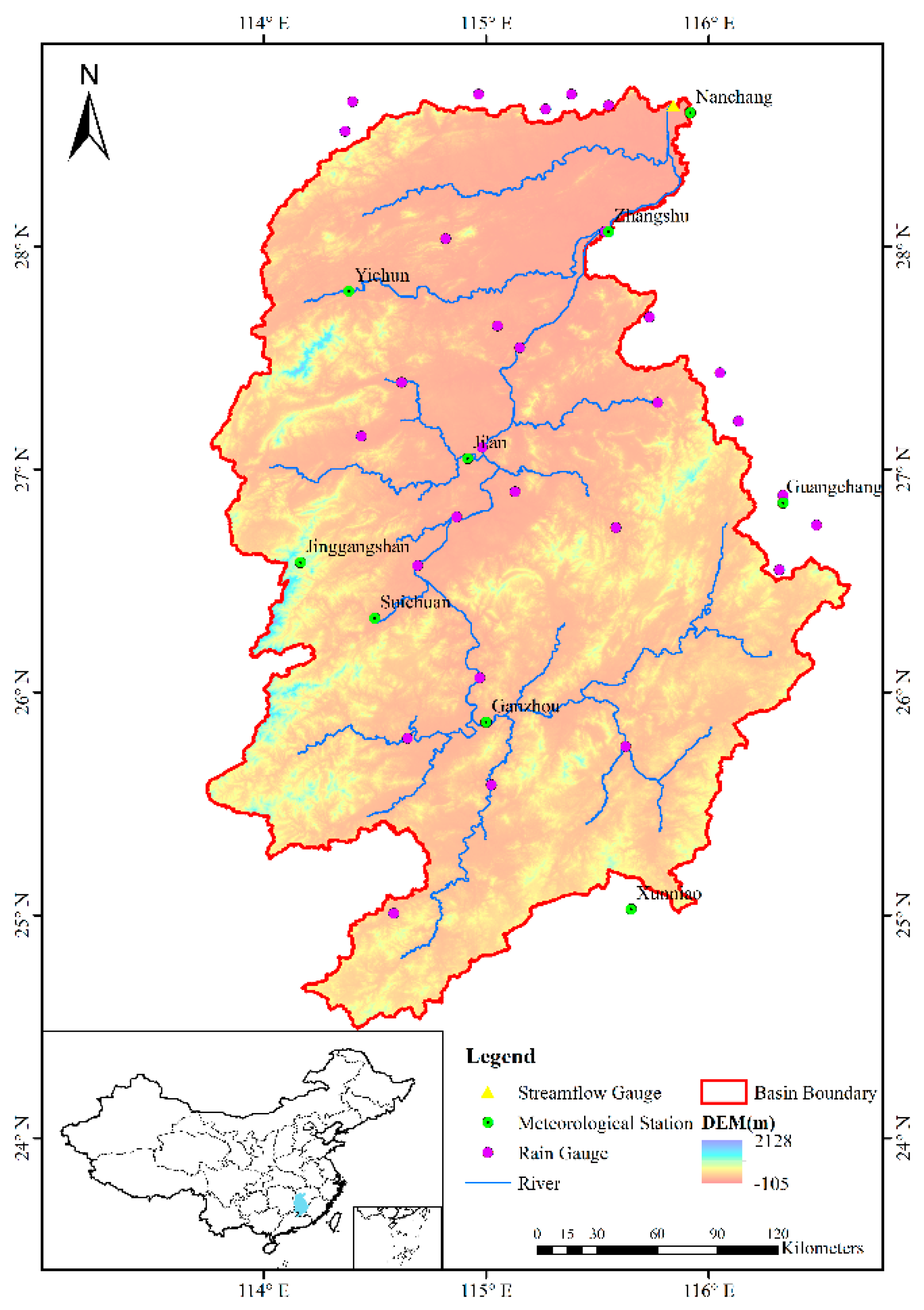
Ganjiang River, with total length of 766 km, is the seventh largest tributary of Yangtze River and also the longest river in Jiangxi province of China. The Ganjiang River Basin (GRB), located within 113°30′~116°40′ E and 24°29′~29°21′ N, covers a total drainage area of 80,948 km2 above Waizhou hydrological station and accounts for 51% of the area of Jiangxi province in the southeast of China (Figure 1). The topography of GRB varies from hills in the southern region to alluvial plains in the northeastern region, with elevation ranging from 105 m below the sea level to 2128 m above the sea level.
The GRB has a typical subtropical humid monsoon climate dominated by East Asian monsoon, and is one of the typical rainstorm regions in China [34]. Due to the comprehensive influences caused by climate and complex terrain, the annual precipitation of GRB is between 1400 and 1600 mm, and the mean annual air temperature is around 17.8 °C. The lowest and highest temperatures are about −5.9 and 39.5 °C, respectively. Because of the monsoon climate and local topography, the precipitation exhibits strongly seasonal and heterogeneous characteristics, with over 70% of the total rainfall concentrating in plum rain season (from April to June).
3. Data and Methodology
3.1. Data
3.1.1. China Meteorological Assimilation Driving Datasets for the SWAT Model (CMADS)
CMADS, developed by Meng et al. [35], is a newly developed meteorological dataset for driving distributed hydrological models such as SWAT [36], Variable Infiltration Capacity (VIC) [37] and Distributed Time-Variant Gain Model (DTVGM) [38,39]. CMADS is constructed by fusing muti-source data on the China Meteorological Administration Land Data Assimilation System (CLDAS). These datasets for constructing CMADS consist of ground-based observed data, satellite monitoring data and numerical products. Compared with satellite datasets such as TMPA or PRESIANN, CMADS can provide multiple meteorological elements, including daily maximum/minimum temperature, daily accumulative precipitation, daily average relative humidity, daily average wind speed and daily accumulative solar radiation. Among these meteorological elements, precipitation and temperature (maximum/minimum or average) play important roles in driving distributed hydrological models. Therefore, it is essential to evaluate the accuracy of precipitation and temperature for CMADS in a given region. The CMADS dataset can provide a high temporal resolution at the daily scale from 2008 to 2016, and cover the whole East Asian region (0°~65° N, 60°~160° E) at 0.333, 0.25, 0.125 and 0.0624 degrees in CMADS V1.0, CMADS V1.1, CMADS V1.2 and CMADS V1.3, respectively. Until now, the application of the CMADS dataset has gained attention from a number of researchers and studies when carrying out water resource modeling, evaluating non-point source pollution, analyzing meteorological data and so on. For example, Meng et al. [28] evaluated the accuracy of CMADS in the mainland of China and applied CMADS in the streamflow forecast of Heihe River Basin, China. The CMADS dataset was also applied in Manas River Basin [40], Yurungkax River Basin [41], Hunhe River Basin [42] and Longnan District [43] in China. In order to compare this dataset with widely used grid satellite products such as TMPA 3B42 or PERSIANN, the CMADS V1.1 with spatial resolution at 0.25 degrees and daily temporal resolution was selected in this study, and this dataset is freely available from Cold and Arid Regions Sciences Data Center at Lanzhou, China (http://westdc.westgis.ac.cn). The CMADS V1.1 with spatial range between 0°~65° N, 60°~160° E, consisting of 400 × 260 (total 10,400) grid points, provides high-quality and high-resolution meteorological data for the investigation of hydrology and meteorology in the East Asian region.
3.1.2. Tropical Rainfall Measuring Mission Multi-Satellite Precipitation Analysis (TMPA)
The Tropical Rainfall Measuring Mission (TRMM) Multi-Satellite Precipitation Analysis (TMPA) with the first space-borne precipitation radar has provided a range of precipitation products since 1997 [44]. TMPA precipitation data have been widely used in many applications, such as hydrological modeling [45], flood prediction [46], drought monitoring [47] and probable maximum precipitation estimation [11]. The latest version (Version 7) of the TMPA products was posted on public websites on 22 May 2012. The TMPA Version 7 has two datasets with daily precipitation estimation. The first is TMPA 3B42RT V7 (hereafter called 3B42RT), the real-time version, which can be obtained around 6–9 h after the observation, and the second is TMPA 3B42 V7 (hereafter called 3B42), the research version, which is freely available approximately two months after the observation. Previous studies have proven that the post-real-time version (3B42) has more accurate and better performance than the real-time version (3B42RT) when carrying out hydro-climate analysis and modeling [10,48]. The difference between these two products is due to the fact that the 3B42 product combines satellite and ground-observed data, including infrared GOES-W (Geostationary Operational Environmental Satellite-West), GOES-E (East), GMS (Geostationary Meteorological Satellite), Meteosat-5, Meteosat-7 and NOAA (National Oceanic and Atmospheric Administration)-12 geostationary satellites, as well as passive microwave radiometers from TMI/TRMM (TRMM Microwave Imager), SSMI/DMSP (Special Sensor Microwave Imager/Defense Meteorological Satellite Program), AMSU/NOAA (Advanced Microwave Sounding Unit/National Oceanic and Atmospheric Administration) and AMSR-E/Aqua (Advanced Microwave Scanning Radiometer-EOS) low-orbit satellites [49]. Therefore, in order to evaluate the performance of satellite products for hydro-climate application, the 3B42 and 3B42RT daily precipitation products were used in this study. The spatial boundary of 3B42 is between 50° S and 50° N with 0.25 degrees spatial resolution, and the temporal extent is from 1998 to now with daily precipitation. Whereas, 3B42RT with spatial extent between 60° S and 60° N can be obtained from March 2000 to now. For the purpose of comparing CMADS, 3B42 and 3B42RT, these two TMPA daily precipitation products ranging from 2008 to 2014 were selected in this study. The TMPA products can be obtained from Goddard Earth Sciences Data and Information Services Center (http://mirador.gsfc.nasa.gov).
3.1.3. Ground-Based Gauge Data
Daily precipitation data of the GRB from 2008 to 2014 were collected from rain gauges and meteorological stations, and daily maximum temperature and minimum temperature data in this region during the same time period were only provided by meteorological stations. The data from 36 rain gauges was obtained from the Hydrology Bureau of Jiangxi Province in China and the data from 9 meteorological gauges can be downloaded from the National Climate Center (NCC) of the China Meteorological Administration (CMA, http://data.cma.cn). The rainfall series of each rain gauge in the GRB has passed the quality control and homogeneity test, which is investigated by Xiao et al. [50]. In addition, daily streamflow data from 2008 to 2014 at the Waizhou hydrological station located in the GRB was also collected from the Hydrology Bureau of Jiangxi Province for calibration and validation of hydrological models. All these data used in this study have been confirmed to be reliable and applicable for driving hydrological models by previous studies [51].
3.1.4. Geospatial Data
In order to drive the distributed hydrological model, a digital elevation model (DEM), a land use map and a soil type map should be firstly prepared in advance. A 3 arc-second (90 m) DEM map of the GRB comes from the Shuttle Radar Topographic Mission (SRTM) Digital Elevation Database of USGS/NASA (United States Geological Survey/National Aeronautics and Space Administration) (http://srtm.csi.cgiar.org). The land use and soil type map with spatial resolution of 1 km were obtained from the Data Center Resources and Environment Sciences, Chinese Academy of Sciences (RESDC, http://www.resdc.cn). The associated soil database contains detailed information about physical soil attributes of different soil layers.
3.2. Statistical Metrics
A set of statistical metrics were selected to evaluate the performance of CMADS, 3B42 and 3B42RT against gauge observations at annual, monthly and daily scales in this study, and these metrics have been widely used for accuracy evaluation of GCPs in previous studies [11,17,33,52,53,54,55]. The continuous statistical metrics consist of the Correlation Coefficient (CC), Root-Mean-Square Error (RMSE), Mean Error (ME) and Relative Bias (BIAS), the categorical statistical metrics include the Probability of Detection (POD), False Alarm Ratio (FAR) and Critical Success Index (CSI), and the SPAtial EFficiency (SPAEF) [56] is used to evaluate the performance of GCPs in spatial pattern matching. Among these statistical metrics, CC was used to evaluate the agreement between CMADS, 3B42, 3B42RT and ground-based observation data, and RMSE, ME and BIAS were used to describe the error and bias of CMADS, 3B42 and 3B42RT [53,54]. POD, FAR and CSI can usually reflect the consistency between CMADS, 3B42, 3B42RT and gauge data. The POD represents the ratio of events correctly detected by satellite or reanalysis products, the FAR refers to the ratio of events falsely reported by these products and the CSI as a function of POD and FAR provides more balanced judgment of satellite or reanalysis products [33,55]. The SPAEF, a relatively new spatial efficiency metric, combines three independent components (correlation, variance and histogram overlap) into one metric and can be applied for spatial similarity evaluation [56,57]. These statistical metrics can be measured as follows:
where n is the number of samples, Si and Gi are the GCPs estimation and ground-based observation values for precipitation or temperature respectively, and are their mean values respectively, H is correct detection (the observed precipitation by gauge that is detected by GCPs correctly), M is missed detection (observed precipitation not detected), F is false alarm (precipitation is not observed in rain gauge, but detected falsely), β is the spatial variability and γ is the overlap between the histograms of GCPs estimation and ground-based observation values. A further description of SPAEF is provided by Demirel et al. [56].
According to Shen et al. [58], the accuracy assessment of these satellite or reanalysis products is largely influenced by the density and distribution of local station networks. Therefore, the point-to-pixel assessment was applied in this study, which means that only the grids with at least one ground-observed station are assessed. In addition, this point-to-pixel assessment approach could avoid adding any additional errors and uncertainties arising from the interpolation process of rain gauges [59].
3.3. Soil and Water Assessment Tools (SWAT)
The SWAT model, developed by the US Department of Agriculture—Agriculture Research Service (USDA-ARS), is a watershed-scale, distributed and physically based hydrological model for simulating the hydrological processes (e.g., runoff, sediment and nutrient transport) and evaluating the influence of different land management practices on these processes in large complex watersheds with various soil types, land use and management conditions over long time periods [36]. Until now, the SWAT model has been one of the most extensively used hydrological models, and lots of studies have proven the capacity of the SWAT model for hydrological simulation and water resources management. In SWAT, a watershed is firstly divided into multiple sub-watersheds based on the information of DEM. Then, each sub-watershed will be further delineated into hydrological response units (HRUs) according to the threshold vales of land use, soil and slope. These threshold values could be set by users to create the HRUs. Each HRU is assumed to be a smaller lumped computing unit with homogeneous land use, soil characteristics, slope and management conditions. In each HRU, most of the hydrological processes in SWAT are carried out at this level and water budget is also simulated at HRU before runoff routing. Then, discharge and pollutant exports of HRUs in a given sub-watershed are aggregated together into the stream network at the outlet of this sub-watershed, and finally routed into the watershed outlet. Further detailed information about the theory, input requirements and output options of SWAT are given in online documents (https://swat.tamu.edu/documentation/2012-io/).
3.4. Input Scenarios Setting and SWAT Model Calibration
This study chose the simulation period from 2008 to 2014, with the first year used for model warming-up. The calibration period was from 2009 to 2011, and years 2012 to 2014 were used to validate the calibrated model. In order to compare the performance of CMADS, 3B42, 3B42RT and gauge-observed data for streamflow simulation, eight input scenarios were set as input for the SWAT model, with detailed information shown in Table 1. The first four scenarios were constructed by combining different sources of precipitation with gauge-observation temperature data, while the remainder of these scenarios used CMADS as the temperature data source. After running the SWAT model with different input scenarios, the applicability of the CMADS, 3B42 and 3B42RT were assessed by comparing the performance of these scenarios.
The SWAT model is calibrated by using the Sequential Uncertainty Fitting algorithm (SUFI-2) within the SWAT Calibration and Uncertainty Programs (SWAT-CUP), which provides a flexible algorithm to calibrate the SWAT model with a large number of input parameters [60]. Based on local knowledge and the previous studies of the SWAT model, ten parameters were selected to calibrate the SWAT model [31,33]. These selected parameters are CN2 (initial SCS runoff curve number for moisture condition II), ESCO (soil evaporation compensation factor), SLSUBBSN (average slope length), CH_N2 (Manning’s n value for the main channel), CH_K2 (effective hydraulic conductivity in main channel alluvium), GWQMN (threshold depth of water in the shallow aquifer required for return flow to occur), REVAPMN (threshold depth of water in the shallow aquifer for “revap” or percolation to the deep aquifer to occur), GW_REVAP (groundwater “revap” coefficient), GW_DELAY (groundwater delay time) and ALPHA_BF (baseflow alpha factor). The sensitivity analysis was also carried out in the SWAT-CUP software to analyze which parameter or what kind of parameters was most sensitive under different input scenarios.
4. Results
4.1. Evaluation and Comparison for Precipitation
4.1.1. Basic Statistical Metrics of CMADS and TMPA against Gauged Precipitation
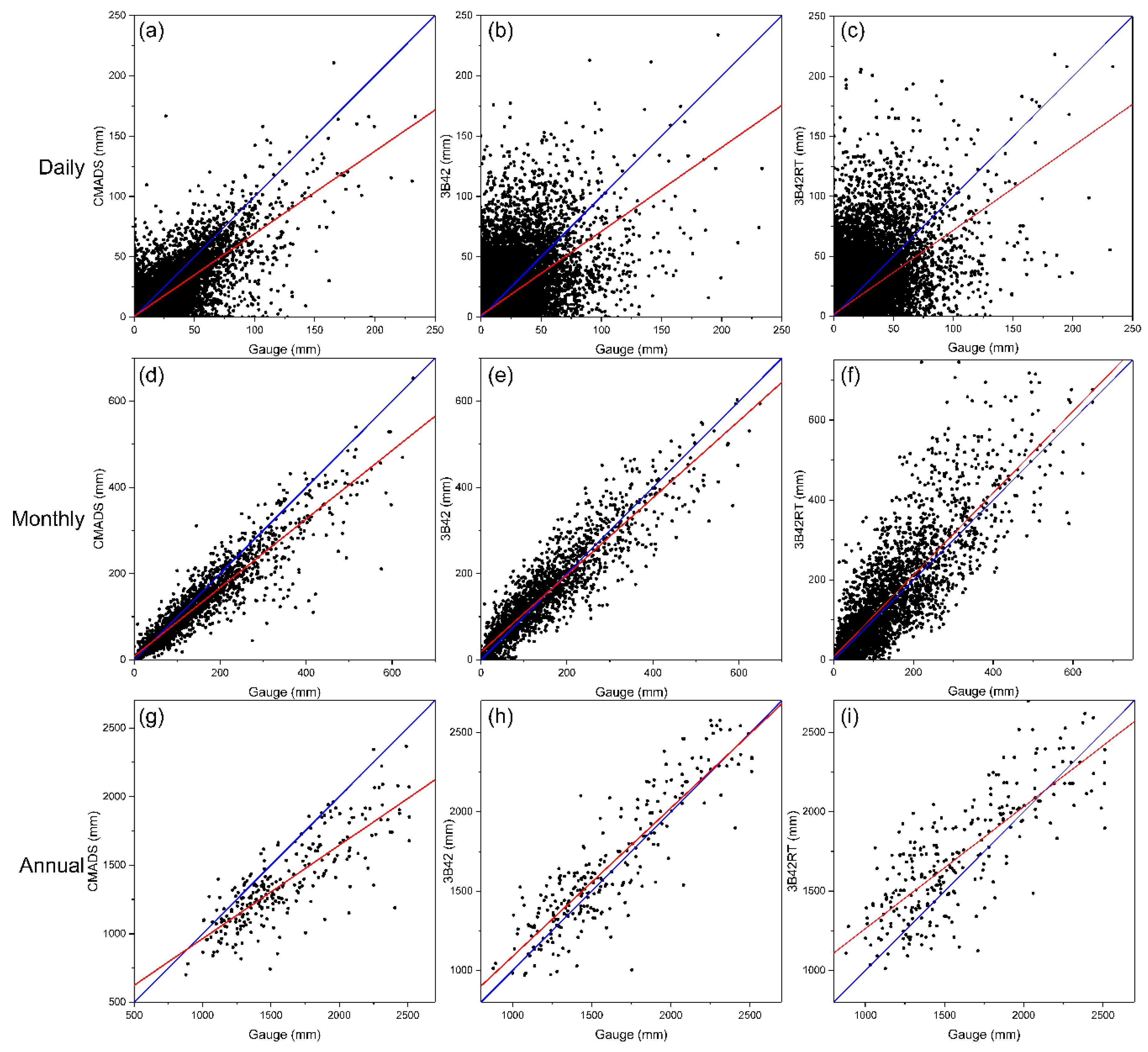
In order to analyze the effect of different precipitation inputs on hydrological simulation, the accuracy of satellite or reanalysis precipitation should be firstly evaluated against ground-based observations. The statistical assessment was computed at 36 pixels with rain gauges, which are considered as the most accurate estimated values of precipitation. The results of the statistical assessment for CMADS, 3B42 and 3B42RT from year 2008 to 2014 at daily, monthly and annual scales are listed in Table 2. In general, each of the three products showed different performances for precipitation estimation at different time scales. At the daily scale, the CMADS obtained the highest CC (0.83) and RMSE (6.35 mm) values among these three products, while 3B42RT had the worst performance with CC and RMSE values of 0.60 and 11.04 mm. However, the ME (−0.60 mm) and RB (−13.37%) of CMADS were obviously worse than those of 3B42 and 3B42RT. It is clear that the CMADS precipitation shows better linear correlation but also significantly underestimates the actual precipitation at the daily time scale. Similar results were obtained at the monthly time scale, but the difference between CMADS, 3B42 and 3B42RT was obviously reduced compared with the daily scale (Table 2). However, the statistical results of values with CC (0.85), RMSE (283.57 mm) and ME (−218.55 mm) for CMADS were worse than results of values with CC (0.90), RMSE (188.27 mm) and ME (58.13 mm) for 3B42 at the annual scale, which is contrary to the performance of these two products at daily and monthly scales. The RMSE and ME values of 3B42RT were obviously better than those of CMADS, although CC of 3B42RT was slightly lower than that of CMADS. In addition, the POD (0.90) and CSI (0.71) of CMADS were significantly higher than those of 3B42 and 3B42RT.
Comprehensively considering the statistical results of CC, RMSE, POD and FAR, the CMADS showed better performance at daily and monthly precipitation estimation, while the 3B42 showed the best performance at annual precipitation estimation. Besides, the same conclusion can be obtained according to ME and RB. It is clear that the 3B42 precipitation slightly overestimated the precipitation and 3B42RT obviously overestimated precipitation based on the respective positive and negative signs for the ME and RB statistical metrics, while the CMADS precipitation resulted in highly underestimated precipitation in the GRB. That is the potential cause of worst performance for CMADS precipitation estimations at the annual scale, at which the total amount of precipitation is more concerned than the seasonal distribution of precipitation.
The precipitation estimated by CMADS, 3B42 and 3B42RT were compared with gauged-based observations at pixels with rain gauges, as shown in Figure 2. This Figure showed that the best-fit line of CMADS (red line in Figure 2a,d,g) is obviously deviating from the diagonal line that we believe could be the best fitted results. Compared with the best-fit line of 3B42 (red line in Figure 2b, e, h) and 3B42RT (red line in Figure 2c,f,i), the CMADS significantly underestimated the precipitation, especially at the annual scale. However, the CMADS precipitation showed better consistency with gauge observations, while the 3B42 and 3B42RT precipitation was more scattered, which was the same with the analysis in Table 2.
4.1.2. Spatial Validation of CMADS and TMPA Precipitation
Actually, precipitation is characterized by highly temporal and spatial variability, which is influenced by climate processes and regional complex topology. Therefore, the spatial assessment of CMADS, 3B42 and 3B42RT should be carried out to analyze the accuracy of these three products. The SPAEF values between ground-based observation and GCPs estimated mean daily, monthly and annual precipitation in GRB are summarized in Table 3. The SPAEF can have a value ranging from −∞ to 1, where a value closer to 1 indicates higher spatial similarity between the ground-based observation and GCPs. The CMADS showed the highest spatial similarity with the highest SPAEF values at daily, monthly, and annual temporal scales, followed by 3B42, and 3B42RT showed the worst spatial similarity based on the SPAEF values. With the temporal resolution extending from daily to monthly and annual scales, the difference between CMADS, 3B42 and 3B42RT was reduced according to the SPAEF values in Table 3.
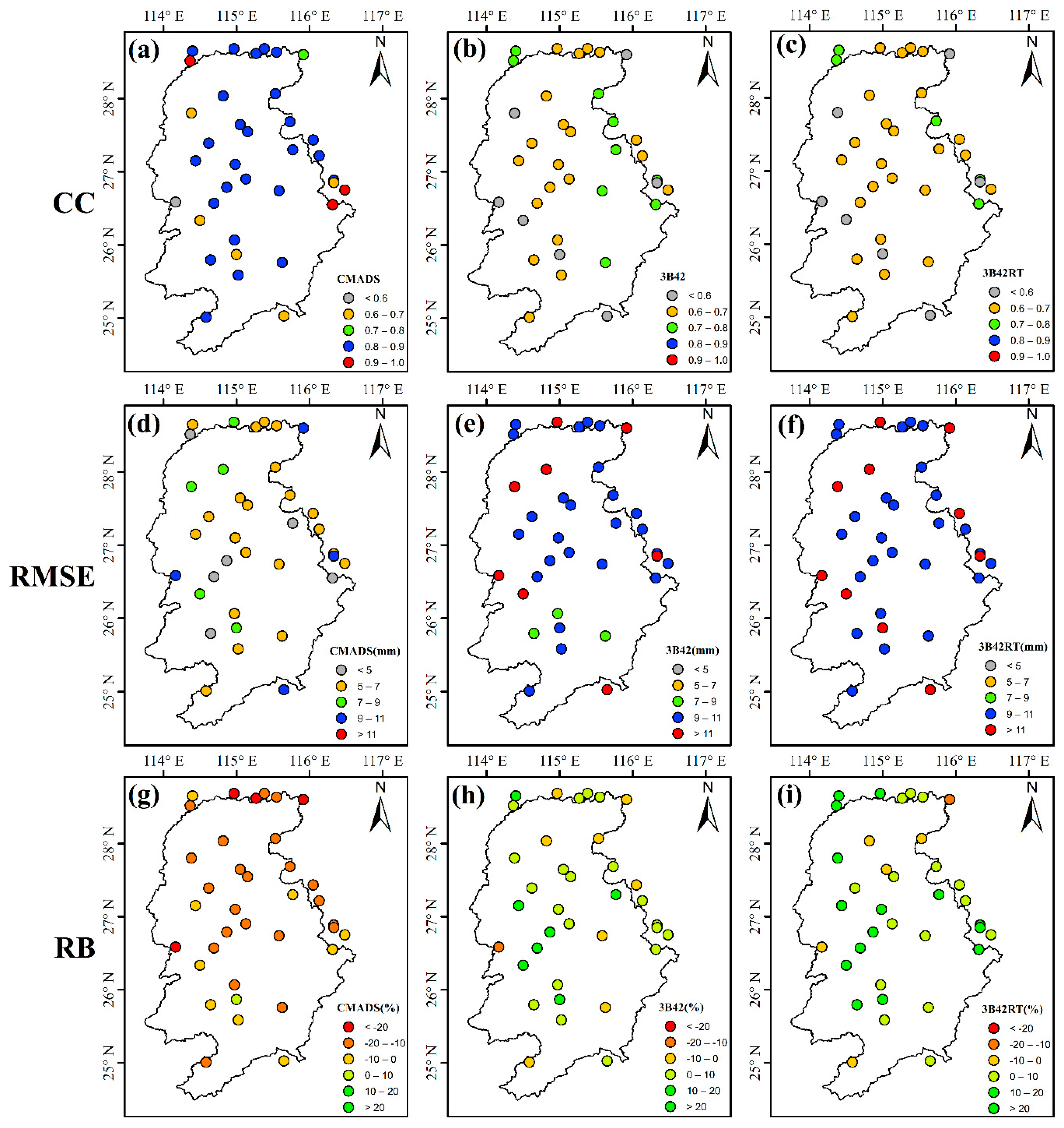
The CC, RMSE and RB values for CMADS, 3B42 and 3B42RT at the daily temporal scale over the whole basin are presented in Figure 3. Compared with 3B42 and 3B42RT, the CMADS showed best performance with highest CC value and lowest RMSE value, which is the same as the SPAEF results. The 3B42 and 3B42RT presented similar spatial characteristics of CC and RMSE, but 3B42 was better for most pixels. As for RB (Figure 3g,h,i), it is clear that the CMADS precipitation significantly underestimated the precipitation at almost all pixels with rain gauges, while the 3B42 and 3B42RT overestimated the precipitation at pixels with rain gauges.
Based on the comprehensive evaluation of CMADS, 3B42 and 3B42RT precipitation at different scales, these three products provided acceptable results in the GRB, but there are some differences between them. The CMADS precipitation can provide more accurate estimation at daily and monthly scales with higher CC, POD and CSI, while the 3B42 is more accurate at the annual time scale with the best CC and RB. This might be due to the difference of precipitation estimation algorithms between them. The satellite precipitation algorithms of 3B42 and 3B42RT can capture strong, extreme precipitation events, but tend to miss shallow precipitation events [30,61], which caused the relatively low POD and CSI values in Table 2. In addition, compared with 3B42RT, 3B42 precipitation data is corrected to reduce the bias by using the GPCC monthly gauge observation [20]. Therefore, 3B42 showed satisfied precipitation estimation at monthly and annual scales, while 3B42RT had a significant overestimation of precipitation.
4.2. Evaluation and Comparison for Temperature of CMADS Dataset
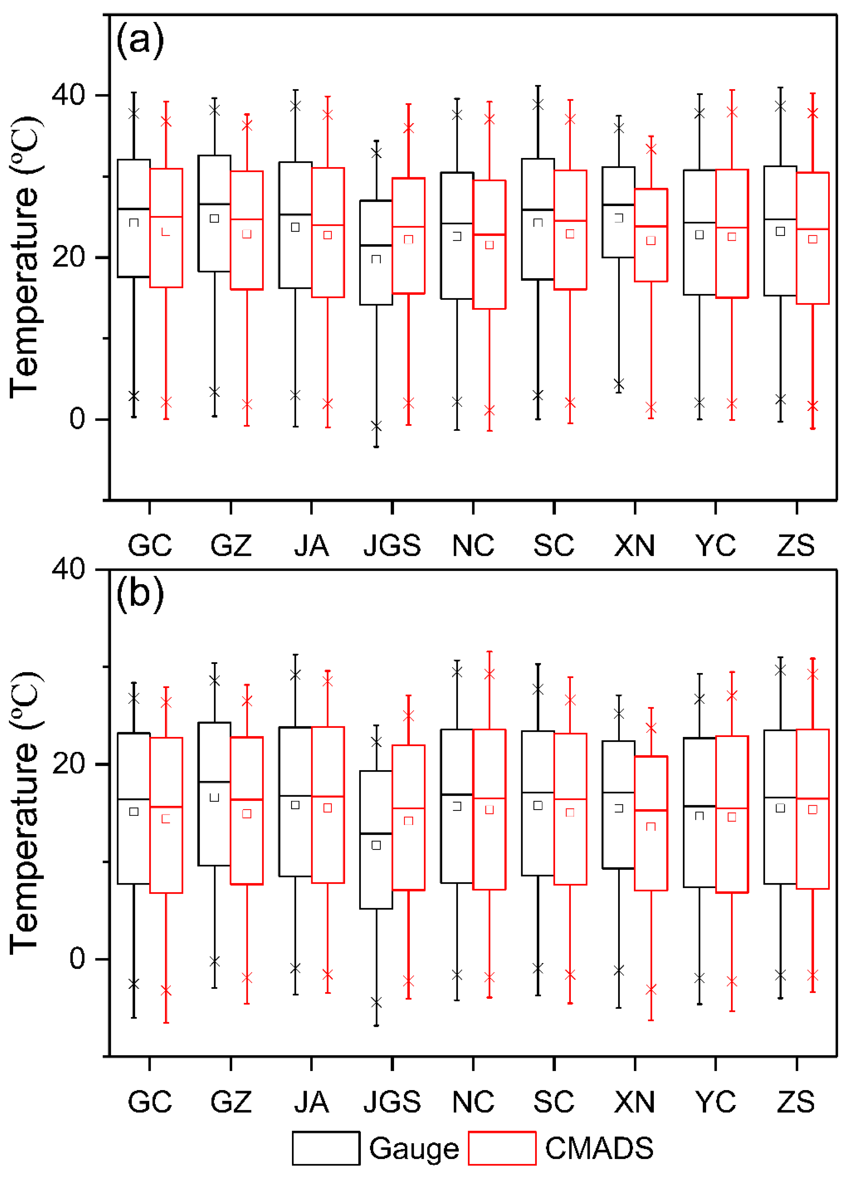
Table 4 lists the statistical assessment results of the CMADS daily maximum and minimum temperature against ground-observation temperature at nine meteorological stations (Figure 1) in the GRB. The comparisons were calculated at nine pixels with meteorological station, from which the most accurate and reliable temperature data can be observed. In general, the CMADS temperature presented highly linear correlation with ground-based observations, with CC values larger than 0.97 for both daily maximum and minimum temperature. In Table 4, the CC values of daily maximum temperature are larger than 0.99 at all meteorological stations, while CC values for most stations are approximately 0.98 when assessing daily minimum temperature. Therefore, the daily maximum temperature estimated by CMADS revealed a better correlation with ground-based observations compared with daily minimum temperature estimation. In addition, all stations except Suichuan and Xunniao stations obtained smaller RMSE for maximum temperature estimation compared with minimum temperature estimation, which showed better estimation for daily maximum temperature.
The box plots of temperature estimated by gauge observations and CMADS at nine meteorological stations in the GRB are shown in Figure 4a for daily maximum temperature and Figure 4b for daily minimum temperature. As shown in Figure 4, the CMADS temperature showed similar statistical characteristics (e.g., mean, median, interquartile range) with ground-based data for both daily maximum and minimum temperature. All stations except Jinggangshan station tended to underestimate the maximum and minimum temperature values, which could also be concluded by analyzing respective positive and negative signs for the ME and RB statistical metrics summarized in Table 3. The different performance for Jinggangshan station could be due to the complex terrains. The Jinggangshan station is located at a mountainous region, in which installation and management of the ground-based stations is difficult and expensive. Therefore, complex terrains and limited data observations in these mountainous regions might affect the performance of CMADS in temperature estimation.
4.3. Performance of SWAT Model Driven by Different Input Scenarios
Before the streamflow simulation results under different input scenarios are presented, the model evaluation criteria should be firstly determined to assess the performance of simulations. For hydrological simulations, the common goals are to maximize the accuracy and reliability of results [62]. For example, the shape and volume of the simulated streamflow hydrograph should be basically the same as those of the observed streamflow process for a given watershed [39]. Therefore, two evaluation criteria, Nash-Sutcliffe efficiency (NSE) [63] and regression coefficient of determination (R2), were selected to evaluate the model performance in this study [64]. NSE reflects fitting degree between simulated streamflow and observed data, while R2 is used to indicate the measured and observed variables [65]. Until now, the absolute criteria for judging model performance have not been established. However, the NSE values greater than 0.75 indicate very good performance, and the values between 0.75 and 0.36 show satisfactory results, while values lower than 0.36 indicate the model has failed to be applied [66].
Based on our local knowledge and a literature review of SWAT in the monsoon region, 10 sensitive parameters were selected for model calibration between 2009 and 2011 and validation between 2012 and 2014. The SWAT model driven by different input scenarios was calibrated with daily streamflow data by using the SUFI-2 algorithm in SWAT-CUP software. Table 5 lists the best fitted calibration parameters and their sensitive ranking under four input scenarios with different precipitation data sources. It is found that there is a difference between the best fitted model parameters driven by different input scenarios. Compared with the parameter sensitive ranking of models driven by observed precipitation (Obs + Obs), the models driven by CMADS (CMADS + Obs) and 3B42 (3B42 + Obs) presented similar sensitive ranking results. All three models identified ALPHA_BF and CN2 as the first two most sensitive parameters. However, the model with 3B42RT as input (3B42RT + Obs) recognized ALPHA_BF and ESCO as the first two most sensitive parameters. Moreover, the sensitive analysis results of the last model were obviously different than the former three models.
The streamflow simulation results were obtained by running the SWAT model with different input scenarios and corresponding parameter values. Generally, the SWAT simulation results based on the ground-observed data (Obs + Obs) agreed well with the observed streamflow during both the calibration and validation periods (Figure 5). As shown in Table 6, the NSE values of the SWAT model driven by observed data (Obs + Obs) were 0.918 and 0.851 for the calibration and validation periods, and the corresponding R2 were 0.919 and 0.867, respectively. The statistical results of NSE and R2 indicated that the SWAT model performed well for hydrological simulation in the GRB according to previously suggested criteria. The simulation results and corresponding statistical metrics of the SWAT model driven by CMADS, 3B42 and 3B42RT precipitation are also shown in Figure 5 and Table 6. For the SWAT simulations driven by CMADS, 3B42 precipitation tended to underestimate the high streamflow and overestimate the low streamflow. The most accurate model simulation results were obtained by driving ground-based precipitation, followed by driving CMADS, 3B42 and 3B42RT precipitation data.
According to the model evaluation criteria discussed above, all the SWAT simulation results driven by CMADS, 3B42 and 3B42RT precipitation data were acceptable, as reflected by the NSE values greater than 0.36 in calibration and validation periods. However, compared with the simulations driven by 3B42 (3B42 + Obs) and 3B42RT (3B42RT + Obs), the model driven by CMADS (CMADS + Obs) with NSE values of 0.873 and 0.778 in calibration and validation periods showed a better alternation for the ground-based observation data. Besides, the simulation results of the CMADS-driven model could capture the relationship between precipitation and streamflow and then obtain better streamflow simulation results, especially for the peak values. The model with 3B42 as input resulted in relatively high underestimation of peak streamflow and overestimation of low streamflow. However, the consistency between simulated streamflow driven by 3B42RT and observed streamflow was worse than results driven by other input scenarios. The R2 values of the CMADS-driven model were 0.875 and 0.837 during calibration and validation periods, which showed the simulation results tracked the observed streamflow better than simulation results with TMPA products as input (Figure 5).
The simulations with CMADS as a temperature data source were also executed for evaluating the influence of different temperature sources on hydrological simulations. Table 6 presents statistical indices (NSE and R2) of SWAT simulations based on different inputs by combing ground-based, CMADS, 3B42 and 3B42RT precipitation with CMADS temperature. Generally, the combination of CMADS temperature with different precipitation sources (Obs + CMADS, CMADS + CMADS, 3B42 + CMADS and 3B42RT + CMADS, in Table 1) as model inputs did not cause much significant difference for the hydrological simulations compared to the simulations driven by observed temperature data and different precipitation sources (Obs + Obs, CMADS + Obs, 3B42 + Obs and 3B42RT + Obs) as input. For example, the model parameters with ground-based precipitation and temperature (Obs + Obs) as input are almost the same with those parameters obtained by ground-based precipitation and CMADS temperature (Obs + CMADS) as input. Furthermore, the differences of calibration and validation NSE values between these two input scenarios are 0.003 and 0.001, respectively. Similar results can be obtained by comparing other input scenarios. It is obvious that the influence of precipitation on the local hydrological cycle is much more significant than that of temperature data in the GRB. This could be due to the high quality of CMADS temperature data and the climatic characteristics of GRB. As shown in Table 4 and Figure 4, the CMADS temperature data showed high consistency with gauge-based observation data, which indicated that CMADS can better capture the temporal and spatial characteristics of temperature. Therefore, the model simulation results with CMADS temperature as inputs showed slight improvement compared to the simulations with ground-based temperature as inputs. On the other hand, the changes of temperature could have a great influence on potential evapotranspiration (e.g., Penman-Monteith method [67]) and snow melts (e.g., degree-day model [68]) processes. However, the GRB is a typical monsoon climatic watershed in southern China, and the hydrological cycle in this region is mainly influenced by the relationship between rainfall and runoff.
5. Discussion
The simulation results of a given hydrological model are mainly dominated by inputs, model structure and model parameters. Inappropriate input data, wrong model structure and erroneous parameter values could obtain a seemingly good simulation [63]. Therefore, the statistical evaluation of CMADS, 3B42 and 3B42RT data was firstly carried out in this study before applying them in any hydrological models. CMADS, 3B42 and 3B42RT precipitation data were evaluated with ground-based data from multiple time scales by using the point-to-pixel method. CMADS temperature evaluation was performed at nine meteorological stations. Then, eight input scenarios by combining four precipitation data (ground-based, CMADS, 3B42 and 3B42RT) with two temperature data (ground-based and CMADS) were set to drive the SWAT model.
From the view of statistical evaluation and hydrological simulation results, the CMADS product has better performance than the 3B42 and 3B42RT products for hydro-climatic analysis. This is due to the differences between the three products’ development processes. The 3B42RT is a real-time precipitation estimation product without correcting by ground-based observation data. However, the precipitation gauge data are applied into the CMADS and 3B42 products. Although both CMADS and 3B42 products have been corrected by ground data, the used land surface observation stations for these two products are different in the mainland of China. The CMADS was developed by fusing satellite observation, numerical products, 40,000 area encryption stations and 2700 national automatic weather stations. In addition, Meng et al. [28,35] found that the CMADS can reflect the temporal and spatial distribution of land surface elements by comparing the CMADS dataset with meteorological elements from 2421 national automatic stations of China Meteorological Administration, which is consistent with the results obtained in this study. However, only about 500 stations in China are utilized to correct the TMPA datasets [69,70], which limits the performance of TMPA products for hydrological and meteorological application in China.
As shown in Table 4 and Figure 4, the temperature of CMADS showed high consistency with ground-based observation data, which provides a potential alternative for hydrological application, especially in ungauged or data-limited basins of China. The CMADS product could reflect the spatial distribution of temperature and improve the accuracy of hydrological simulation, which is significant for the mountainous basins and alpine regions with sparse monitoring networks. Several studies have been conducted in these regions by using the CMADS product, such as Heihe River Basin [35], Mannas River Basin [40], Yurungkax River Basin [41], Hunhe River Basin [42] and Longnan District [43] in China.
In the present study, the hydrological evaluation of GCPs was conducted only by one distributed hydrological model, SWAT. However, different hydrological models have their own model structures, complexities and process presentations. Therefore, choosing only one model would cause a relatively larger deviation than using multiple models in the hydrological evaluation of GCPs. Besides the datasets (CMADS, 3B42 and 3B42RT) used in this study, there are lots of satellite-based precipitation products and reanalysis products, such as Climate Hazards Group Infrared Precipitation with Station data (CHIRPS) [71], Integrated Multi-SatellitE Retrievals for the Global Precipitation Measurement (GPM) mission (IMERG) [72], PERSIANN-CDR, CMORPH, Asian Precipitation-Highly-Resolved Observational Data Integration Towards Evaluation (APHRODITE) [73], NCEP-CFSR, CMADS, ERA−5 [74], etc. For the future work, it will be better to compare these regional products with more global datasets, and to investigate how to merge these different products into one more reliable and accurate dataset.
In general, East Asia is a part of the largest continent in the world, with about 1.5 billion inhabitants. The complex monsoon climate and highly heterogeneous terrains result in large climate variations [28]. However, the lack of meteorological data from ground-based stations limits the hydro-climatic application and also brings more uncertainty for driving the complex distributed hydrological models when using these limited data. In this study, the CMADS, 3B42 and 3B42RT datasets provide a potential alternative for driving hydrological models or conducting basin water balance analysis.
6. Conclusions
This study evaluated the precipitation of CMADS, 3B42 and 3B42RT against the ground-based observation data in the Ganjiang River Basin, China. Daily maximum and minimum temperatures of CMADS were compared with these meteorological elements at nine meteorological stations. Then, eight input scenarios by combining four precipitation datasets (ground-based, CMADS, 3B42 and 3B42RT) with two temperature datasets (ground-based, CMADS) were applied to force the SWAT model. The SWAT simulation results driven by different input scenarios were compared and analyzed to estimate the influence of different inputs on hydrological simulation. The main conclusions are as follows.
The CMADS, 3B42 and 3B42RT datasets showed acceptable performance for precipitation estimation in the GRB. The CMADS precipitation presented best estimation with ground-based observation precipitation at daily and monthly scales, while 3B42 was better in estimating annual precipitation. The CMADS tended to underestimate precipitation, the 3B42 showed a slight overestimation of precipitation, while 3B42RT obviously overestimated precipitation. The CMADS precipitation with high accuracy has huge potentiality for watershed hydrological modeling, especially in the ungauged or data-limited regions. For the temperature, the CMADS showed highly linear correlation with ground-based observations, which provides a potential source of temperature data for hydrological modeling.
Eight input scenarios were set to force the distributed hydrological model, SWAT. Different input scenarios resulted in different best-fitted values of model parameters. The streamflow simulations driven by CMADS showed better replication of observed streamflow than that driven by 3B42 and 3B42RT. In addition, CMADS could capture the spatial distribution characteristics of temperature well. We recommend the integration of different precipitation data with CMADS temperature data for hydrological modeling in China, especially in the mountainous basins and alpine regions. In conclusion, CMADS, 3B42 and 3B42RT can capture the precipitation and temperature, and can be well applied in hydrological simulation. Satellite and reanalysis products provide valuable data for hydro-climatic analysis in ungauged or data-limited basins.
Author Contributions
Conceptualization, J.X. and Q.W.; methodology, X.Z., Q.W., and J.L.; software, Q.W.; validation, Q.W. and P.L.; data curation, J.L.; original draft preparation, Q.W.; review and editing, D.S., Q.W., and J.L. All authors have read and agreed to the published version of the manuscript.
Funding
This research was funded by the National Key Research and Development Program of China (No. 2016YFC0402709), the National Natural Science Foundation of China (No. 41890823), and the Strategic Priority Research Program of the Chinese Academy of Sciences (grant no. XDA23040304).
Acknowledgments
The authors’ gratitude is extended to the China Meteorological Administration for providing ground-based precipitation. The research community of CMADS and TMPA products are also highly appreciated for developing the free data for international users. The authors gratefully acknowledged the valuable comments and suggestions given by the editors and the anonymous reviewers.
Conflicts of Interest
The authors declare no conflict of interest.
References
- McCabe, G.J.; Wolock, D.M. Variability and Trends in Runoff Efficiency in the Conterminous United States. J. Am. Water Resour. Assoc. 2016, 52, 1046–1055. [Google Scholar] [CrossRef]
- Schneider, U.; Ziese, M.; Meyer-Christoffer, A.; Finger, P.; Rustemeier, E.; Becker, A. The new portfolio of global precipitation data products of the Global Precipitation Climatology Centre suitable to assess and quantify the global water cycle and resources. Proc. Int. Assoc. Hydrol. Sci. 2016, 374, 29–34. [Google Scholar] [CrossRef] [Green Version]
- Daly, C.; Slater, M.E.; Roberti, J.A.; Laseter, S.H.; Swift, L.W. High-resolution precipitation mapping in a mountainous watershed: Ground truth for evaluating uncertainty in a national precipitation dataset. Int. J. Climatol. 2017, 37, 124–137. [Google Scholar] [CrossRef] [Green Version]
- Held, I.M.; Soden, B.J. Robust responses of the hydrological cycle to global warming. J. Clim. 2006, 19, 5686–5699. [Google Scholar] [CrossRef]
- Zhang, X.; Tang, Q.; Zhang, X.; Lettenmaier, D.P. Runoff sensitivity to global mean temperature change in the CMIP5 Models. Geophys. Res. Lett. 2014, 41, 5492–5498. [Google Scholar] [CrossRef]
- Wang, W.; Wei, J.; Shao, Q.; Xing, W.; Yong, B.; Yu, Z.; Jiao, X. Spatial and temporal variations in hydro-climatic variables and runoff in response to climate change in the Luanhe River basin, China. Stoch. Environ. Res. Risk Assess. 2015, 29, 1117–1133. [Google Scholar] [CrossRef]
- Woodhouse, C.A.; Pederson, G.T.; Morino, K.; McAfee, S.A.; McCabe, G.J. Increasing influence of air temperature on upper Colorado River streamflow. Geophys. Res. Lett. 2016, 43, 2174–2181. [Google Scholar] [CrossRef] [Green Version]
- Salio, P.; Hobouchian, M.P.; García Skabar, Y.; Vila, D. Evaluation of high-resolution satellite precipitation estimates over southern South America using a dense rain gauge network. Atmos. Res. 2015, 163, 146–161. [Google Scholar] [CrossRef]
- Tauro, F.; Selker, J.; Van De Giesen, N.; Abrate, T.; Uijlenhoet, R.; Porfiri, M.; Manfreda, S.; Caylor, K.; Moramarco, T.; Benveniste, J.; et al. Measurements and observations in the XXI century (MOXXI): Innovation and multi-disciplinarity to sense the hydrological cycle. Hydrol. Sci. J. 2018, 63, 169–196. [Google Scholar] [CrossRef] [Green Version]
- Tan, M.L.; Ibrahim, A.L.; Duan, Z.; Cracknell, A.P.; Chaplot, V. Evaluation of six high-resolution satellite and ground-based precipitation products over Malaysia. Remote Sens. 2015, 7, 1504–1528. [Google Scholar] [CrossRef] [Green Version]
- Yang, Y.; Tang, G.; Lei, X.; Hong, Y.; Yang, N. Can satellite precipitation products estimate probable maximum precipitation: A comparative investigation with gauge data in the Dadu River basin. Remote Sens. 2018, 10, 41. [Google Scholar] [CrossRef] [Green Version]
- van de Giesen, N.; Hut, R.; Selker, J. The Trans-African Hydro-Meteorological Observatory (TAHMO). Wiley Interdiscip. Rev. Water 2014, 1, 341–348. [Google Scholar] [CrossRef] [Green Version]
- Feki, H.; Slimani, M.; Cudennec, C. Geostatistically based optimization of a rainfall monitoring network extension: Case of the climatically heterogeneous Tunisia. Hydrol. Res. 2017, 48, 514–541. [Google Scholar] [CrossRef]
- Gosset, M.; Kunstmann, H.; Zougmore, F.; Cazenave, F.; Leijnse, H.; Uijlenhoet, R.; Chwala, C.; Keis, F.; Doumounia, A.; Boubacar, B.; et al. Improving rainfall measurement in gauge poor regions thanks to mobile telecommunication networks. Bull. Am. Meteorol. Soc. 2016, 97, ES49–ES51. [Google Scholar] [CrossRef]
- Stokstad, E. Scarcity of rain, stream gages threatens forecasts. Science 1999, 285, 1199–1200. [Google Scholar] [CrossRef]
- Seyyedi, H.; Anagnostou, E.N.; Beighley, E.; McCollum, J. Satellite-driven downscaling of global reanalysis precipitation products for hydrological applications. Hydrol. Earth Syst. Sci. 2014, 18, 5077–5091. [Google Scholar] [CrossRef] [Green Version]
- Tong, K.; Su, F.; Yang, D.; Hao, Z. Evaluation ofsatellite precipitation retrievals and their potential utilities in hydrologic modeling over the Tibetan Plateau. J. Hydrol. 2014, 519, 423–437. [Google Scholar] [CrossRef]
- McCabe, M.F.; Rodell, M.; Alsdorf, D.E.; Miralles, D.G.; Uijlenhoet, R.; Wagner, W.; Lucieer, A.; Houborg, R.; Verhoest, N.E.C.; Franz, T.E.; et al. The future of Earth observation in hydrology. Hydrol. Earth Syst. Sci. 2017, 21, 3879–3914. [Google Scholar] [CrossRef] [Green Version]
- Beck, H.E.; Vergopolan, N.; Pan, M.; Levizzani, V.; Van Dijk, A.I.J.M.; Weedon, G.P.; Brocca, L.; Pappenberger, F.; Huffman, G.J.; Wood, E.F. Global-scale evaluation of 22 precipitation datasets using gauge observations and hydrological modeling. Hydrol. Earth Syst. Sci. 2017, 21, 6201–6217. [Google Scholar] [CrossRef] [Green Version]
- Huffman, G.J.; Bolvin, D.T.; Nelkin, E.J.; Wolff, D.B.; Adler, R.F.; Gu, G.; Hong, Y.; Bowman, K.P.; Stocker, E.F. The TRMM Multisatellite Precipitation Analysis (TMPA): Quasi-Global, Multiyear, Combined-Sensor Precipitation Estimates at Fine Scales. J. Hydrometeorol. 2007, 8, 38–55. [Google Scholar] [CrossRef]
- Joyce, R.J.; Janowiak, J.E.; Arkin, P.A.; Xie, P. CMORPH: A Method that Produces Global Precipitation Estimates from Passive Microwave and Infrared Data at High Spatial and Temporal Resolution. J. Hydrometeorol. 2004, 5, 487–503. [Google Scholar] [CrossRef]
- Ashouri, H.; Hsu, K.L.; Sorooshian, S.; Braithwaite, D.K.; Knapp, K.R.; Cecil, L.D.; Nelson, B.R.; Prat, O.P. PERSIANN-CDR: Daily precipitation climate data record from multisatellite observations for hydrological and climate studies. Bull. Am. Meteorol. Soc. 2015, 96, 69–83. [Google Scholar] [CrossRef] [Green Version]
- Saha, S.; Moorthi, S.; Pan, H.L.; Wu, X.; Wang, J.; Nadiga, S.; Tripp, P.; Kistler, R.; Woollen, J.; Behringer, D.; et al. The NCEP climate forecast system reanalysis. Bull. Am. Meteorol. Soc. 2010, 91, 1015–1057. [Google Scholar] [CrossRef]
- Schamm, K.; Ziese, M.; Becker, A.; Finger, P.; Meyer-Christoffer, A.; Schneider, U.; Schröder, M.; Stender, P. Global gridded precipitation over land: A description of the new GPCC First Guess Daily product. Earth Syst. Sci. Data 2014, 6, 49–60. [Google Scholar] [CrossRef] [Green Version]
- Huffman, G.J.; Adler, R.F.; Morrissey, M.M.; Bolvin, D.T.; Curtis, S.; Joyce, R.; McGavock, B.; Susskind, J. Global Precipitation at One-Degree Daily Resolution from Multisatellite Observations. J. Hydrometeorol. 2001, 2, 36–50. [Google Scholar] [CrossRef] [Green Version]
- Weedon, G.P.; Gomes, S.; Viterbo, P.; Shuttleworth, W.J.; Blyth, E.; Österle, H.; Adam, J.C.; Bellouin, N.; Boucher, O.; Best, M. Creation of the WATCH Forcing Data and Its Use to Assess Global and Regional Reference Crop Evaporation over Land during the Twentieth Century. J. Hydrometeorol. 2011, 12, 823–848. [Google Scholar] [CrossRef] [Green Version]
- Harris, I.; Jones, P.D.; Osborn, T.J.; Lister, D.H. Updated high-resolution grids of monthly climatic observations—The CRU TS3.10 Dataset. Int. J. Climatol. 2014, 34, 623–642. [Google Scholar] [CrossRef] [Green Version]
- Meng, X.; Wang, H. Significance of the China meteorological Assimilation Driving Datasets for the SWAT model (CMADS) of East Asia. Water 2017, 9, 765. [Google Scholar] [CrossRef]
- Li, L.; Xu, C.Y.; Zhang, Z.; Jain, S.K. Validation of a new meteorological forcing data in analysis of spatial and temporal variability of precipitation in India. Stoch. Environ. Res. Risk Assess. 2014, 28, 239–252. [Google Scholar] [CrossRef]
- Chen, S.; Hong, Y.; Cao, Q.; Tian, Y.; Hu, J.; Zhang, X.; Li, W.; Carr, N.; Shen, X.; Qiao, L. Intercomparison of precipitation estimates from WSR-88D radar and TRMM measurement over continental United States. IEEE Trans. Geosci. Remote Sens. 2015, 53, 4444–4456. [Google Scholar] [CrossRef]
- Tuo, Y.; Duan, Z.; Disse, M.; Chiogna, G. Evaluation of precipitation input for SWAT modeling in Alpine catchment: A case study in the Adige river basin (Italy). Sci. Total Environ. 2016, 573, 66–82. [Google Scholar] [CrossRef] [PubMed] [Green Version]
- Lauri, H.; Räsänen, T.A.; Kummu, M. Using Reanalysis and Remotely Sensed Temperature and Precipitation Data for Hydrological Modeling in Monsoon Climate: Mekong River Case Study. J. Hydrometeorol. 2014, 15, 1532–1545. [Google Scholar] [CrossRef]
- Tan, M.L.; Gassman, P.W.; Cracknell, A.P. Assessment of three long-term gridded climate products for hydro-climatic simulations in tropical river basins. Water 2017, 9, 229. [Google Scholar] [CrossRef] [Green Version]
- Tang, G.; Zeng, Z.; Long, D.; Guo, X.; Yong, B.; Zhang, W.; Hong, Y. Statistical and Hydrological Comparisons between TRMM and GPM Level-3 Products over a Midlatitude Basin: Is Day-1 IMERG a Good Successor for TMPA 3B42V7? J. Hydrometeorol. 2016, 17, 121–137. [Google Scholar] [CrossRef]
- Meng, X.; Wang, H.; Cai, S.; Zhang, X.; Leng, G. The China Meteorological Assimilation Driving Datasets for the SWAT Model ( CMADS ) Application in China: A Case Study in Heihe River Basin. Preprints 2016. [Google Scholar] [CrossRef] [Green Version]
- Arnold, J.G.; Srinivasan, R.; Muttiah, R.S.; Williams, J.R. Large Area Hydrologic Modeling and Assessment Part I: Model Development. J. Am. Water Resour. Assoc. 1998, 34, 73–89. [Google Scholar] [CrossRef]
- Liang, X.; Lettenmaier, D.P.; Wood, E.F.; Burges, S.J. A simple hydrologically based model of land surface water and energy fluxes for general circulation models. J. Geophys. Res. 1994, 99, 14415. [Google Scholar] [CrossRef]
- XIA, J. Development of distributed time-variant gain model for nonlinear hydrological systems. Sci. China Ser. D 2005, 48, 713. [Google Scholar] [CrossRef]
- Xia, J.; Wang, Q.; Zhang, X.; Wang, R.; She, D. Assessing the influence of climate change and inter-basin water diversion on Haihe River basin, eastern China: A coupled model approach. Hydrogeol. J. 2018, 26, 1455–1473. [Google Scholar] [CrossRef]
- Meng, X.; Wang, H.; Lei, X.; Cai, S.; Wu, H.; Ji, X.; Wang, J. Hydrological modeling in the Manas River Basin using soil and water assessment tool driven by CMADS. Teh. Vjesn. Tech. Gaz. 2017, 24, 525–534. [Google Scholar]
- Liu, J.; Liu, S.; Shangguan, D.; Xu, J. Applicability Evaluation of Precipitation Datasets from CMADS, ITPCAS and TRMM 3B42 in Yurungkax River Basin. J. N. China Univ. Water Resour. Eletr. Power (Nat. Sci. Ed.) 2017, 38, 28–37. (In Chinese) [Google Scholar]
- Zhang, L.; Wang, H.; Meng, X. Application of SWAT Model Driven by CMADS in Hunhe River Basin in Liaoning Province. J. N. China Univ. Water Resour. Eletr. Power (Nat. Sci. Ed.) 2017, 38, 1–9. (In Chinese) [Google Scholar]
- Tian, F.; Zhang, J.; Ran, Y.; Liu, J.; Liu, S. Assessment of Debris Flow Disaster Hazard and Influence Factors in Longnan District. J. Catastrophol. 2017, 32, 197–203. (In Chinese) [Google Scholar]
- Kummerow, C.; Simpson, J.; Thiele, O.; Barnes, W.; Chang, A.T.C.; Stocker, E.; Adler, R.F.; Hou, A.; Kakar, R.; Wentz, F.; et al. The status of the Tropical Rainfall Measuring Mission (TRMM) after two years in orbit. J. Appl. Meteorol. 2000, 39, 1965–1982. [Google Scholar] [CrossRef]
- Su, F.; Hong, Y.; Lettenmaier, D.P. Evaluation of TRMM Multisatellite Precipitation Analysis (TMPA) and its utility in hydrologic prediction in the La Plata Basin. J. Hydrometeorol. 2008, 9, 622–640. [Google Scholar] [CrossRef] [Green Version]
- Nanda, T.; Sahoo, B.; Beria, H.; Chatterjee, C. A wavelet-based non-linear autoregressive with exogenous inputs (WNARX) dynamic neural network model for real-time flood forecasting using satellite-based rainfall products. J. Hydrol. 2016, 539, 57–73. [Google Scholar] [CrossRef]
- Levina; Hatmoko, W.; Seizarwati, W.; Vernimmen, R. Comparison of TRMM satellite rainfall and APHRODITE for drought analysis in the Pemali-Comal River Basin. In Proceedings of the 2nd International Symposium on Lapan-Ipb Satellite (Lisat) for Food Security and Environmental Monitoring, Bogor, India, 25–26 October 2016; Setiawan, Y., Prasetyo, L.B., Siregar, I.Z., Effendi, H., Eds.; Elsevier Science BV: Amsterdam, The Netherlands, 2016; Volume 33, pp. 187–195. [Google Scholar]
- Jiang, S.; Zhang, Z.; Huang, Y.; Chen, X.; Chen, S. Evaluating the TRMM Multisatellite Precipitation Analysis for Extreme Precipitation and Streamflow in Ganjiang River Basin, China. Adv. Meteorol. 2017, 2017. [Google Scholar] [CrossRef]
- Ringard, J.; Becker, M.; Seyler, F.; Linguet, L. Temporal and spatial assessment of four satellite rainfall estimates over French Guiana and north Brazil. Remote Sens. 2015, 7, 16441–16459. [Google Scholar] [CrossRef] [Green Version]
- Xiao, Y.; Zhang, X.; Wan, H.; Wang, Y.; Liu, C.; Xia, J. Spatial and temporal characteristics of rainfall across Ganjiang River Basin in China. Meteorol. Atmos. Phys. 2016, 128, 167–179. [Google Scholar] [CrossRef]
- Zhang, L.; Lu, J.; Chen, X.; Liang, D.; Fu, X.; Sauvage, S.; Perez, J.M.S. Stream flow simulation and verification in ungauged zones by coupling hydrological and hydrodynamic models: A case study of the Poyang Lake ungauged zone. Hydrol. Earth Syst. Sci. 2017, 21, 5847–5861. [Google Scholar] [CrossRef] [Green Version]
- Tan, M.L.; Samat, N.; Chan, N.W.; Roy, R. Hydro-meteorological assessment of three GPM Satellite Precipitation Products in the Kelantan River Basin, Malaysia. Remote Sens. 2018, 10, 1011. [Google Scholar] [CrossRef] [Green Version]
- Lo Conti, F.; Hsu, K.L.; Noto, L.V.; Sorooshian, S. Evaluation and comparison of satellite precipitation estimates with reference to a local area in the Mediterranean Sea. Atmos. Res. 2014, 138, 189–204. [Google Scholar] [CrossRef] [Green Version]
- Liu, J.; Xia, J.; She, D.; Li, L.; Wang, Q.; Zou, L. Evaluation of Six Satellite-Based Precipitation Products and Their Ability for Capturing Characteristics of Extreme Precipitation Events over a Climate Transition Area in China. Remote Sens. 2019, 11, 1477. [Google Scholar] [CrossRef] [Green Version]
- Ebert, E.E.; Janowiak, J.E.; Kidd, C. Comparison of near-real-time precipitation estimates from satellite observations and numerical models. Bull. Am. Meteorol. Soc. 2007, 88, 47–64. [Google Scholar] [CrossRef] [Green Version]
- Demirel, M.C.; Mai, J.; Mendiguren, G.; Koch, J.; Samaniego, L.; Stisen, S. Combining satellite data and appropriate objective functions for improved spatial pattern performance of a distributed hydrologic model. Hydrol. Earth Syst. Sci. 2018, 22, 1299–1315. [Google Scholar] [CrossRef] [Green Version]
- Ahmed, K.; Sachindra, D.A.; Shahid, S.; Demirel, M.C.; Chung, E.-S. Selection of multi-model ensemble of general circulation models for the simulation of precipitation and maximum and minimum temperature based on spatial assessment metrics. Hydrol. Earth Syst. Sci. 2019, 23, 4803–4824. [Google Scholar] [CrossRef] [Green Version]
- Shen, Y.; Xiong, A.; Wang, Y.; Xie, P. Performance of high-resolution satellite precipitation products over China. J. Geophys. Res. Atmos. 2010, 115. [Google Scholar] [CrossRef]
- Dembélé, M.; Zwart, S.J. Evaluation and comparison of satellite-based rainfall products in Burkina Faso, West Africa. Int. J. Remote Sens. 2016, 37, 3995–4014. [Google Scholar] [CrossRef] [Green Version]
- Abbaspour, K.C.; Rouholahnejad, E.; Vaghefi, S.; Srinivasan, R.; Yang, H.; Kløve, B. A continental-scale hydrology and water quality model for Europe: Calibration and uncertainty of a high-resolution large-scale SWAT model. J. Hydrol. 2015, 524, 733–752. [Google Scholar] [CrossRef] [Green Version]
- Klein Tank, A.M.G.; Zwiers, F.W.; Zhang, X. Guidelines on Analysis of Extremes in a Changing Climate in Support of Informed Decisions for Adaptation; World Meteorological Organization: Geneva, Switzerland, 2009. [Google Scholar]
- Duan, Q.; Ajami, N.K.; Gao, X.; Sorooshian, S. Multi-model ensemble hydrologic prediction using Bayesian model averaging. Adv. Water Resour. 2007, 30, 1371–1386. [Google Scholar] [CrossRef] [Green Version]
- Nash, J.E.; Sutcliffe, J.V. River Flow Forecasting Through Conceptual Models Part I-a Discussion of Principles. J. Hydrol. 1970, 10, 282–290. [Google Scholar] [CrossRef]
- Moriasi, D.N.; Arnold, J.G.; van Liew, M.W.; Bingner, R.L.; Harmel, R.D.; Veith, T.L. Model Evaluation Guidelines for Systematic Quantification of Accuracy in Watershed Simulations. Trans. ASABE 2007, 50, 885–900. [Google Scholar] [CrossRef]
- Schaefli, B.; Gupta, H.V. Do Nash values have value? Hydrol. Process. 2007, 21, 2075–2080. [Google Scholar] [CrossRef] [Green Version]
- Krause, P.; Boyle, D.P.; Bäse, F. Comparison of different efficiency criteria for hydrological model assessment. Adv. Geosci. 2005, 5, 89–97. [Google Scholar] [CrossRef] [Green Version]
- Allen, R.G.; Pereira, L.S.; Raes, D.; Smith, M. Crop evapotranspiration—Guidelines for computing crop water requirements—FAO Irrigation and drainage paper 56. Irrig. Drain. 1998, 56, 1–15. [Google Scholar]
- Hock, R. Temperature index melt modelling in mountain areas. J. Hydrol. 2003, 282, 104–115. [Google Scholar] [CrossRef]
- Chen, S.; Hong, Y.; Cao, Q.; Gourley, J.J.; Kirstetter, P.; Yong, B.; Tian, Y.; Zhang, Z.; Shen, Y.; Hu, J.; et al. Similarity and difference of the two successive V6 and V7 TRMM multisatellite precipitation analysis performance over China. J. Geophys. Res. Atmos. 2014, 118, 1–15. [Google Scholar] [CrossRef]
- Liu, S.; Yan, D.; Qin, T.; Weng, B.; Li, M. Correction of TRMM 3B42V7 Based on Linear Regression Models over China. Adv. Meteorol. 2016, 2016. [Google Scholar] [CrossRef]
- Funk, C.; Peterson, P.; Landsfeld, M.; Pedreros, D.; Verdin, J.; Shukla, S.; Husak, G.; Rowland, J.; Harrison, L.; Hoell, A.; et al. The climate hazards infrared precipitation with stations-a new environmental record for monitoring extremes. Sci. Data 2015, 2, 150066. [Google Scholar] [CrossRef] [Green Version]
- Huffman, G.J.; Bolvin, D.T.; Nelkin, E.J.; Tan, J. Integrated Multi-satellitE Retrievals for GPM (IMERG) technical documentation. NASA/GSFC Code 2015, 612, 47. [Google Scholar]
- Yatagai, A.; Kamiguchi, K.; Arakawa, O.; Hamada, A.; Yasutomi, N.; Kitoh, A. APHRODITE: Constructing a long-term daily gridded precipitation dataset for Asia based on a dense network of rain gauges. Bull. Am. Meteorol. Soc. 2012, 93, 1401–1415. [Google Scholar] [CrossRef]
- Hersbach, H.; Bell, B.; Berrisford, P.; Horányi, A.; Sabater, J.M.; Nicolas, J.; Radu, R.; Schepers, D.; Simmons, A.; Soci, C.; et al. Global reanalysis: Goodbye ERA-Interim, hello ERA5. ECMWF Newsl. 2019, 159, 17–24. [Google Scholar]
Figure 1.
Sketch map of the Ganjiang River Basin (GRB) and corresponding rain gauges, meteorological stations and streamflow gauge.
Figure 1.
Sketch map of the Ganjiang River Basin (GRB) and corresponding rain gauges, meteorological stations and streamflow gauge.

Figure 2.
Scatterplots of precipitation comparison at selected pixels with rain gauges for CMADS (left column), 3B42 (middle column) and 3B42RT (right column) in the GRB: (a–c) at the daily time scale, (d–f) at the monthly time scale and (g–i) at the annual time scale. The diagonal line is blue, and the best-fit line estimated by the OLS (ordinary least square) method is red.

Figure 3.
Spatial distribution of statistical metrics at selected pixels with rain gauges for CMADS (left column), 3B42 (middle column) and 3B42 RT (right column) in the GRB: (a–c) CC, (d–f) RMSE and (g–i) RB.
Figure 3.
Spatial distribution of statistical metrics at selected pixels with rain gauges for CMADS (left column), 3B42 (middle column) and 3B42 RT (right column) in the GRB: (a–c) CC, (d–f) RMSE and (g–i) RB.

Figure 4.
Box plots of temperature estimated from meteorological gauges and CMADS in the GRB for (a) daily maximum temperature and (b) daily minimum temperature (GC: Guangchang; GZ: Ganzhou; JA: Jian; JGS: Jianggangshan; NC: Nanchang; SC: Suichuan; XN: Xunnian; YC: Yichun; ZS: Zhangshu, shown in Figure 1).

Figure 5.
Comparison of daily observed streamflow with SWAT-simulated streamflow driven by (a) Obs + Obs, (b) CMADS + Obs, (c) 3B42 + Obs and (d) 3B42RT + Obs input scenarios, respectively.
Figure 5.
Comparison of daily observed streamflow with SWAT-simulated streamflow driven by (a) Obs + Obs, (b) CMADS + Obs, (c) 3B42 + Obs and (d) 3B42RT + Obs input scenarios, respectively.


Table 1.
Input Scenarios setting for the Soil and Water Assessment Tools (SWAT) model.
| Input Scenario | Precipitation | Temperature |
|---|---|---|
| Obs + Obs | Gauge-observed precipitation data | Gauge-observed temperature data |
| 3B42 + Obs | 3B42 precipitation data | Gauge-observed temperature data |
| 3B42RT + Obs | 3B42RT precipitation data | Gauge-observed temperature data |
| CMADS + Obs | CMADS precipitation data | Gauge-observed temperature data |
| Obs + CMADS | Gauge-observed precipitation data | CMADS temperature data |
| 3B42 + CMADS | 3B42 precipitation data | CMADS temperature data |
| 3B42RT + CMADS | 3B42RT precipitation data | CMADS temperature data |
| CMADS + CMADS | CMADS precipitation data | CMADS temperature data |
Note: CMADS = China Meteorological Assimilation Driving Datasets for the SWAT Model; 3B42 = Tropical Rainfall Measuring Mission Multi-Satellite Precipitation Analysis (TMPA) 3B42 V7; 3B42RT = TMPA 3B42RT V7.
Table 2.
Summary of statistical metrics for CMADS and TMPA daily, monthly and annual precipitation in the GRB. The metrics were calculated based on the grids with rain gauges.
Table 2.
Summary of statistical metrics for CMADS and TMPA daily, monthly and annual precipitation in the GRB. The metrics were calculated based on the grids with rain gauges.
| Time | Statistical | Products | ||
|---|---|---|---|---|
| Metrics | CMADS | 3B42 | 3B42RT | |
| Daily | CC | 0.83 ** | 0.63 ** | 0.60 ** |
| RMSE (mm) | 6.35 | 10.3 | 11.04 | |
| ME (mm) | −0.60 | 0.16 | 0.35 | |
| Monthly | CC | 0.94 ** | 0.91 ** | 0.82 ** |
| RMSE (mm) | 41.95 | 42.98 | 74.58 | |
| ME (mm) | −18.21 | 4.84 | 10.79 | |
| Annual | CC | 0.85 ** | 0.90 ** | 0.82 ** |
| RMSE (mm) | 283.57 | 188.27 | 259.79 | |
| ME (mm) | −218.55 | 58.13 | 129.46 | |
| RB (%) | −13.37 | 4.19 | 8.63 | |
| POD | 0.90 | 0.61 | 0.56 | |
| FAR | 0.23 | 0.22 | 0.23 | |
| CSI | 0.71 | 0.52 | 0.48 | |
Note: ** Significant at p < 0.01. CC indicates Correlation Coefficient, RMSE indicates Root-Mean-Square Error, ME indicate Mean Error, RB indicates Relative Bias, POD indicates Probability of Detection, FAR indicates False Alarm Ratio and CSI indicates Critical Success Index.
Table 3.
Summary of SPAtial EFficiency (SPAEF) values for CMADS and TMPA daily, monthly and annual precipitation in the GRB. The metrics were calculated based on the mean precipitation at different temporal scales.
Table 3.
Summary of SPAtial EFficiency (SPAEF) values for CMADS and TMPA daily, monthly and annual precipitation in the GRB. The metrics were calculated based on the mean precipitation at different temporal scales.
| Time | Products | ||
|---|---|---|---|
| CMADS (Rank) | 3B42 (Rank) | 3B42RT (Rank) | |
| Daily | 0.57 (1) | 0.52 (2) | 0.49 (3) |
| Monthly | 0.55 (1) | 0.54 (2) | 0.51 (3) |
| Annual | 0.55 (1) | 0.54 (2) | 0.51 (3) |
Table 4.
Summary of statistical metrics for CMADS daily maximum and minimum temperature in the GRB. The metrics were calculated based on the grids with meteorological stations.
Table 4.
Summary of statistical metrics for CMADS daily maximum and minimum temperature in the GRB. The metrics were calculated based on the grids with meteorological stations.
| Daily Temperature | Station | Statistical Metrics | |||
|---|---|---|---|---|---|
| CC | RMSE (°C) | ME (°C) | RB (%) | ||
| Maximum | Guangchang | 0.99 ** | 1.62 | −1.08 | −4.46 |
| Ganzhou | 0.99 ** | 2.24 | −1.93 | −7.75 | |
| Jian | 0.99 ** | 1.48 | −0.99 | −4.15 | |
| Jinggangshan | 0.99 ** | 2.82 | 2.47 | 12.50 | |
| Nanchang | 0.99 ** | 1.47 | −1.03 | −4.57 | |
| Suichuan | 0.99 ** | 1.86 | −1.36 | −5.58 | |
| Xunnian | 0.99 ** | 3.02 | −2.81 | −11.28 | |
| Yichun | 0.99 ** | 1.30 | −0.26 | −1.14 | |
| Zhangshu | 0.99 ** | 1.43 | −0.96 | −4.14 | |
| Minimum | Guangchang | 0.98 ** | 1.91 | −0.73 | −4.82 |
| Ganzhou | 0.98 ** | 2.35 | −1.69 | −10.19 | |
| Jian | 0.99 ** | 1.53 | −0.31 | −1.96 | |
| Jinggangshan | 0.98 ** | 2.95 | 2.50 | 21.37 | |
| Nanchang | 0.99 ** | 1.56 | −0.34 | −2.17 | |
| Suichuan | 0.98 ** | 1.75 | −0.72 | −4.57 | |
| Xunnian | 0.97 ** | 2.67 | −1.89 | −12.23 | |
| Yichun | 0.98 ** | 1.71 | −0.11 | −0.74 | |
| Zhangshu | 0.98 ** | 1.64 | −0.15 | −1.00 | |
Note: ** Significant at p < 0.01.
Table 5.
Optimal calibration value and sensitive ranking of model parameters under different input scenarios in the Ganjiang River Basin (GRB).
Table 5.
Optimal calibration value and sensitive ranking of model parameters under different input scenarios in the Ganjiang River Basin (GRB).
| Parameter | Range | Obs + Obs | CMADS + Obs | 3B42 + Obs | 3B42RT + Obs | |||||
|---|---|---|---|---|---|---|---|---|---|---|
| Min | Max | Value | Sensitive Ranking | Value | Sensitive Ranking | Value | Sensitive Ranking | Value | Sensitive Ranking | |
| A__CN2 | −20 | 20 | 0.74 | 2 | 18.62 | 2 | 17.22 | 2 | −14.30 | 10 |
| V__ESCO | 0 | 1 | 0.96 | 4 | 0.81 | 3 | 0.06 | 3 | 0.91 | 2 |
| A__SLSUBBSN | −9 | 130 | 11.92 | 10 | −6.57 | 10 | 69.33 | 9 | 93.37 | 9 |
| V__CH_N2 | 0 | 0.3 | 0.26 | 8 | 0.07 | 8 | 0.06 | 10 | 0.08 | 8 |
| V__CH_K2 | 0 | 400 | 327.8 | 3 | 265.8 | 6 | 219.0 | 6 | 331.0 | 5 |
| A__GWQMN | −500 | 500 | −350.5 | 5 | −369.5 | 4 | −269.5 | 4 | 101.5 | 6 |
| A__REVAPMN | −500 | 500 | −396.5 | 7 | −19.5 | 9 | −76.5 | 7 | −67.5 | 4 |
| V__GW_REVAP | 0.02 | 0.2 | 0.11 | 6 | 0.10 | 5 | 0.08 | 5 | 0.07 | 7 |
| V__GW_DELAY | 0 | 300 | 124.05 | 9 | 37.05 | 7 | 263.55 | 8 | 183.15 | 3 |
| V__ALPHA_BF | 0 | 1 | 0.83 | 1 | 0.50 | 1 | 0.47 | 1 | 0.80 | 1 |
Note: A means a given value is added to the existing parameter value, and V indicates the existing parameters value is to be replaced by a given value. CN2 = initial SCS runoff curve number for moisture condition II; ESCO = soil evaporation compensation factor); SLSUBBSN = average slope length; CH_N2 = Manning’s n value for the main channel; CH_K2 = effective hydraulic conductivity in main channel alluvium; GWQMN = threshold depth of water in the shallow aquifer required for return flow to occur; REVAPMN = threshold depth of water in the shallow aquifer for “revap” or percolation to the deep aquifer to occur; GW_REVAP = groundwater “revap” coefficient; GW_DELAY = groundwater delay time; ALPHA_BF = baseflow alpha factor.
Table 6.
Statistical results of the SWAT model during calibration and validation periods driven by different input scenarios in the GRB (input scenarios shown in Table 1).
Table 6.
Statistical results of the SWAT model during calibration and validation periods driven by different input scenarios in the GRB (input scenarios shown in Table 1).
| Input Scenario | Calibration | Validation | ||
|---|---|---|---|---|
| NSE | R2 | NSE | R2 | |
| Obs + Obs | 0.918 | 0.919 | 0.851 | 0.867 |
| 3B42 + Obs | 0.762 | 0.797 | 0.685 | 0.742 |
| 3B42RT + Obs | 0.755 | 0.770 | 0.449 | 0.568 |
| CMADS + Obs | 0.873 | 0.875 | 0.778 | 0.837 |
| Obs + CMADS | 0.921 | 0.921 | 0.852 | 0.868 |
| 3B42 + CMADS | 0.764 | 0.797 | 0.681 | 0.742 |
| 3B42RT + CMADS | 0.758 | 0.771 | 0.447 | 0.570 |
| CMADS + CMADS | 0.873 | 0.874 | 0.784 | 0.837 |
Publisher’s Note: MDPI stays neutral with regard to jurisdictional claims in published maps and institutional affiliations. |
© 2020 by the authors. Licensee MDPI, Basel, Switzerland. This article is an open access article distributed under the terms and conditions of the Creative Commons Attribution (CC BY) license (http://creativecommons.org/licenses/by/4.0/).
Share and Cite
MDPI and ACS Style
Wang, Q.; Xia, J.; Zhang, X.; She, D.; Liu, J.; Li, P. Multi-Scenario Integration Comparison of CMADS and TMPA Datasets for Hydro-Climatic Simulation over Ganjiang River Basin, China. Water 2020, 12, 3243. https://doi.org/10.3390/w12113243
AMA Style
Wang Q, Xia J, Zhang X, She D, Liu J, Li P. Multi-Scenario Integration Comparison of CMADS and TMPA Datasets for Hydro-Climatic Simulation over Ganjiang River Basin, China. Water. 2020; 12(11):3243. https://doi.org/10.3390/w12113243
Chicago/Turabian StyleWang, Qiang, Jun Xia, Xiang Zhang, Dunxian She, Jie Liu, and Pengjun Li. 2020. "Multi-Scenario Integration Comparison of CMADS and TMPA Datasets for Hydro-Climatic Simulation over Ganjiang River Basin, China" Water 12, no. 11: 3243. https://doi.org/10.3390/w12113243
Note that from the first issue of 2016, this journal uses article numbers instead of page numbers. See further details here.