Glacier Mapping Based on Random Forest Algorithm: A Case Study over the Eastern Pamir


School of Spatial Informatics and Geomatics Engineering, Anhui University of Science and Technology, Huainan 232001, China
*
Author to whom correspondence should be addressed.
Water 2020, 12(11), 3231; https://doi.org/10.3390/w12113231
Submission received: 28 September 2020
/
Revised: 11 November 2020
/
Accepted: 16 November 2020
/
Published: 18 November 2020
(This article belongs to the Section Hydrology)
Abstract
:Debris-covered glaciers are common features on the eastern Pamir and serve as important indicators of climate change promptly. However, mapping of debris-covered glaciers in alpine regions is still challenging due to many factors including the spectral similarity between debris and the adjacent bedrock, shadows cast from mountains and clouds, and seasonal snow cover. Considering that few studies have added movement velocity features when extracting glacier boundaries, we innovatively developed an automatic algorithm consisting of rule-based image segmentation and Random Forest to extract information about debris-covered glaciers with Landsat-8 OLI/TIRS data for spectral, texture and temperature features, multi-digital elevation models (DEMs) for elevation and topographic features, and the Inter-mission Time Series of Land Ice Velocity and Elevation (ITS_LIVE) for movement velocity features, and accuracy evaluation was performed to determine the optimal feature combination extraction of debris-covered glaciers. The study found that the overall accuracy of extracting debris-covered glaciers using combined movement velocity features is 97.60%, and the Kappa coefficient is 0.9624, which is better than the extraction results using other schemes. The high classification accuracy obtained using our method overcomes most of the above-mentioned challenges and can detect debris-covered glaciers, illustrating that this method can be executed efficiently, which will further help water resources management.
1. Introduction
Glaciers are important indicators of climate change and play an indispensable role in the global water cycle [1]. In the context of global warming, the global glaciers experienced large-scale glacier melting during 2003–2009, accounting for 29 ± 13% [2] of the global sea-level rise during the same period. Glacier changes in alpine areas of Asia not only contribute to sea-level rise [3], but most importantly, they affect the runoff patterns and sizes of dozens of rivers around alpine areas of Asia [4], which have the largest population density in the world. Besides, in recent years, hydrogeological disasters caused by glacier changes have occurred frequently, threatening the lives and properties of downstream people [5]. Some studies also predict that in the next few decades, glaciers in alpine areas of Asia will continue to decrease [6,7]. Therefore, it is of great significance to study the characteristic of glaciers in alpine areas of Asia.
Accurately extracting glacier areas and monitoring glacier morphology are the basic requirements for glacier research [8]. Currently, with the requirement of glacier inventory establishment and more in-depth research in glaciers, several prominent methods of identifying and classifying glaciers to extract clean glacier boundaries, mainly including artificial visual interpretation [9], the band ratio threshold method [10,11], supervised classification [12], and unsupervised classification [13,14], have been extensively developed. Due to the fact that the band ratio threshold method is the most efficient, least manual intervention, and is more accurate, it has been widely used in glacier inventory and glacier research on a large geographic scale [15,16]. The threshold segmentation method of optical images effectively extracts clean glaciers is well [11], but it remains a tough mission to detect debris-covered glaciers. To date, the automatic identification methods of the debris-covered glaciers include the terrain-based method [17], radar interferometry [18] and thermal infrared remote sensing method [19]. For now, it is unfortunate that detecting the boundary of the debris-covered glaciers based on human visual interpretation has higher accuracy [15,16].
Detecting the boundary of a glacier is challenging due to debris-covered glaciers which have similar spectral characteristics to the adjacent rocky mountain surface, cloud cover, and shadows cast from mountains and clouds and seasonal snow, making identification of the debris-covered glaciers still a harsh task [20], and a defect of the terrain-based method is that areas with no obvious topographical changes compared with glacier areas can be misjudged as glaciers [17,21]. Additionally, the accuracy of the debris boundary extracted by this method also relies on the quality of the DEM and the type of the debris; radar interferometry cannot achieve good results in the identification of small glaciers or glacier boundaries with weak changes [18]; the thermal infrared remote sensing method cannot identify glaciers whose debris thickness exceeds 40–50 m [19]. Another challenge in glacier mapping over the eastern Pamir, where spatial inhomogeneity of the glacial surface remains an obstacle to glacier identification, increasing the difficulty of observing and understanding glacial changes, is enormous due to the cold, dry climate and coupled with high mountains in the southwest; in particular, the distribution of glaciers is mainly affected by clouds and mountain shadows with large areas [15,16]. Most studies in this area [22,23,24] have focused on non-debris-covered glaciers or manual glacier mapping, owing to problems in identifying debris. Therefore, determining how to optimize effective data to automatically classify the presence or absence of debris-covered glaciers needs more thorough and deeper research. Faced with the ever-increasing amount of remote sensing data, making efficient use of remote sensing data is a critical factor in glacier research. However, traditional manual digitization is time-consuming and laborious and has difficulty in application [25,26]. Therefore, it is well worth developing an efficient and high-precision automatic mapping method for glaciers based on remote sensing data [27].
Random Forest is one of the most established algorithms in ensemble learning [28,29]. It can be understood as the organic fusion of Bagging ensemble learning and Decision Tree algorithms [30], which can effectively get over the problem of overfitting to the training data set, thereby improving the accuracy of the classification and the stability of the model. Moreover, compared with traditional machine learning algorithms, Random Forest also has significant advantages in providing generalization and algorithm operational efficiency [31,32]. Random Forest, as an integrated classifier, has a wide range of applications in hydrology, including large-scale discharge simulation [33], short-term daily streamflow forecast [34], groundwater salinity susceptibility mapping [35], river water salinity prediction [36], accurate estimation of groundwater nitrate concentration [37], flood and erosion susceptibility mapping [38], susceptibility mapping of soil water erosion [39], and snow avalanches [40,41]. The studies above show that Random Forest can be successfully developed for geographical datasets.
Zhang [42] took advantage of multi-temporal Landsat imagery and multi-source digital elevation model data, combined with various surface information and the Random Forest method to detect the boundary of debris-covered glaciers, and through the integration of multi-phase image results, the impact of clouds and seasonal snow cover on the classification results is reduced. Hussain and Khan [43] compared Support Vector Machines, Artificial Neural Networks, and Random Forests based on Sentinel-2, Landsat 8, DEM and other data in the study of debris-covered glaciers recognition; Random Forests showed the highest classification accuracy. Alifu [27] contrasted the classification results of the six classifiers of K-NearestNeighbor, Support Vector Machine, Gradient Boosting Tree, Decision Tree, Random Forest and Multi-Layer Perceptron, which showed that the use of Random Forest classifier combined with multi-source remote sensing images obtained the highest classification accuracy, and information on debris-covered glaciers could be accurately obtained. Based on Random Forest methods and satellite remote sensing data, different types of glaciers can be quickly extracted [27,42,43]. However, none of the above studies considered the characteristics of glacier movement.
Landsat-8 satellite data have abundant spectral bands and high spatial resolution that provide multi-dimensional feature space for land cover classification. However, multi-dimensional features participating in classification easily cause information redundancy, leading to reduced classification speed and accuracy [44,45]. Therefore, determining how to make full use of the rich spectral and spatial information of Landsat-8 data and optimising the features through high-dimensional feature space dimensionality reduction is highly significant in improving classification accuracy [46]. The velocity of glacier movement is the result of many internal and external glacial factors [47,48]. Identifying the characteristics of glacier movement velocity is requisite for understanding the spatial distribution of glaciers [49,50]. Introducing the characteristics of glacier movement velocity (ITS_LIVE dataset), which no studies have added, in glacier mapping, and studying the relationship between glacier movement and the surface topography, will steadily help in the further detection of glaciers.
To date, automated methods of glacier boundary mapping are limited to seasonal snow, shadows and debris-covered factors, and manual methods have a high labor cost. The timely acquisition of glacier boundary information using mature automatic glacier boundary extraction methods will provide significant value. Therefore, it is necessary to develop mature automatic glacier boundary extraction methods. Although machine learning has opened up many fields in glacier research, the application of machine learning in the glacier mapping is still rarely seen, and the glacier classification algorithm is relatively simple, which cannot effectively improve the accuracy of automatic glacier classification. Considering the advantages of stable performance of Random Forest algorithm, high classification accuracy and convenience for feature importance evaluation, it was selected as an automatic classification algorithm to extract information about debris-covered glaciers, and accuracy evaluation was performed to determine the optimal feature combination extraction of debris-covered glaciers. We used the eastern Pamir glaciers as an example, classified various types of glaciers and summarised the characteristics and distribution of glaciers.
2. Research Area
The eastern Pamir [51] is situated at the intersection between the southwestern part of the Xinjiang Uygur Autonomous Region of China and the Tarim Basin, which is mainly at the intersection of the Tianshan, Kunlun and Karakorum Mountains, with an average altitude of 3200 to 4500 m. The study area is a subregion of the eastern Pamir (Figure 1) located in the Qinghai–Tibet Plateau, with a geographic location between 38°06′ N–38°46′ N and 75°00′ E–75°31′ E. The glaciers on the remote sensing image are mainly located in the Kongur Tagh where the incline is steep, the altitude generally above 7000 m and the modern snow line approximately 5900 m above sea-level. The great height of these mountains in the eastern Pamir provides a vast accumulation space and hydrothermal conditions for the formation of glaciers and the glaciers are therefore well developed.
3. Datasets
3.1. Pre-Processing
3.1.1. Spectral Features
The Landsat-8 Operational Land Imager (OLI) and Thermal Infrared Sensor (TIRS) scenes of World Reference System 2 (WRS2) path 149 and row 33, acquired on 20 October 2017, with 3.74% cloud coverage, were acquired in GeoTIFF format from the Geospatial Data Cloud site, Computer Network Information Center, Chinese Academy of Sciences. The images were chosen with cloud cover below 10% and were selected at the end of the ablation period in the same year (2017) to minimise the impact of seasonal snow on the mapping of glaciers in the same measurement. In the entire image taken on 20 October 2017, there was almost no cloud cover over the glacier, and therefore this image was selected as the main image of the study and other images were employed to compensate for the impact of mountain shadows and cloud cover [52] (Table 1). The pre-processing of the Landsat-8 OLI image was undertaken with ENVI 5.3 software, including radiometric calibration and atmospheric correction. The spectral reflectance features included seven bands from the Landsat-8 OLI images (Coastal/Aerosol, Blue, Green, Red, NIR, SWIR1 and SWIR2).
Spectral indices features were extracted by calculating the Normalised Difference Vegetation Index (NDVI) [53], Normalised Difference Water Index (NDWI) [54] and Normalised Difference Snow Index (NDSI) [55]. These were calculated as follows:
where , , and are surface reflectance in the green, red, near-infrared and short-wave infrared bands, respectively.
3.1.2. Textural Features
Using the Co-occurrence Measures tool (GLCM), a 3 × 3 window was selected to calculate eight kinds of texture information which, based on the second-order matrix, can be applied. The information included mean, variance, homogeneity, contrast, dissimilarity, and information entropy, second moment and correlation. The computational formulae of these features were defined by Haralick et al. (1973) [56]. They were calculated in sequence as follows:
where and are coordinates of the GLCM, refers to the value at the position in the GLCM and and represent the means and standard deviations of and .
3.1.3. Temperature Features
Land Surface Temperature (LST) plays an important role in energy exchange between the land surface and atmosphere [57]. The ENVI module [58,59] was used to calculate the LST in Landsat 8 TIRS of band10. The LST of Landsat-8 TIRS images was used to calculate the following:
where is the TOA radiance converted from band 10 of Landsat-8, is the TOA brightness temperature converted from the sensor calibration parameters provided in the header file, is the blackbody radiance, which is given by the Planck’s law, is the land surface temperature, is the atmospheric transmittance, is the land surface emissivity, is the down-welling atmospheric radiance, and is the upwelling atmospheric radiance.
3.1.4. Topographic Features
Advanced Spaceborne Thermal Emission and Reflection Radiometer (ASTER) Global Digital Elevation Model Version 2 (GDEM V2) data, derived from multiple ASTER images between 2000 and 2010, had a vertical accuracy of ±15 m and a horizontal resolution of 30 m [60]. The GDEM V2 data were downloaded in GeoTIFF format from the Geospatial Data Cloud site, Computer Network Information Center, Chinese Academy of Sciences. The GDEM V2 data were employed to provide topographic information: elevation, slope, aspect, shaded relief, profile convexity, plan convexity, longitudinal convexity, cross-sectional convexity, minimum curvature, maximum curvature, and root-mean-square error.
3.1.5. Movement Velocity Features
The Inter-mission Time Series of Land Ice Velocity and Elevation (ITS_LIVE) was extracted from NASA’s MEaSUREs project (https://its-live.jpl.nasa.gov/), extracted from Landsat-4, -5, -7 and -8. The glacier data product contained data on all glacial movements and elevation changes from 1985 to 2018. During the processing, Landsat-4 and Landsat-5 images with 1–4 bands, and Landsat-7 and -8 panchromatic bands, were employed to supplement the missing data in Landsat-7 with random data for local normalisation, oversampling, feature tracking, etc., to extract the glacier movement velocity [61]. The data had two resolutions of 120 m and 240 m. The multi-year average data resolution accepted in this study was 120 m, the single-year data resolution was 240 m and the data version employed was V0. The bilinear interpolation method was adopted to resample the ITS_LIVE data to the same resolution as the Landsat-8 data [50].
3.1.6. Verification Features
Additionally, the second glacier inventory dataset of China (version 1.0) (2006–2011) was obtained from the Cold and Arid Regions Sciences Data Center in Lanzhou [15]. Tibetan Plateau glacier data—TPG2017 (version 1.0)—was provided by the National Tibetan Plateau Data Center [24]. The CCI dataset (Glacier inventory of the Pamir and Karakoram) was downloadable [23]. These datasets were applied to estimate the effectiveness of the glacier boundary detection, based on the Random Forest algorithm, in this experiment.
All datasets were projected to the same coordinate system of the 1984 World Geodetic System (WGS 84), with the Universal Transverse Mercator (UTM) Zone 43 North (Table 2).
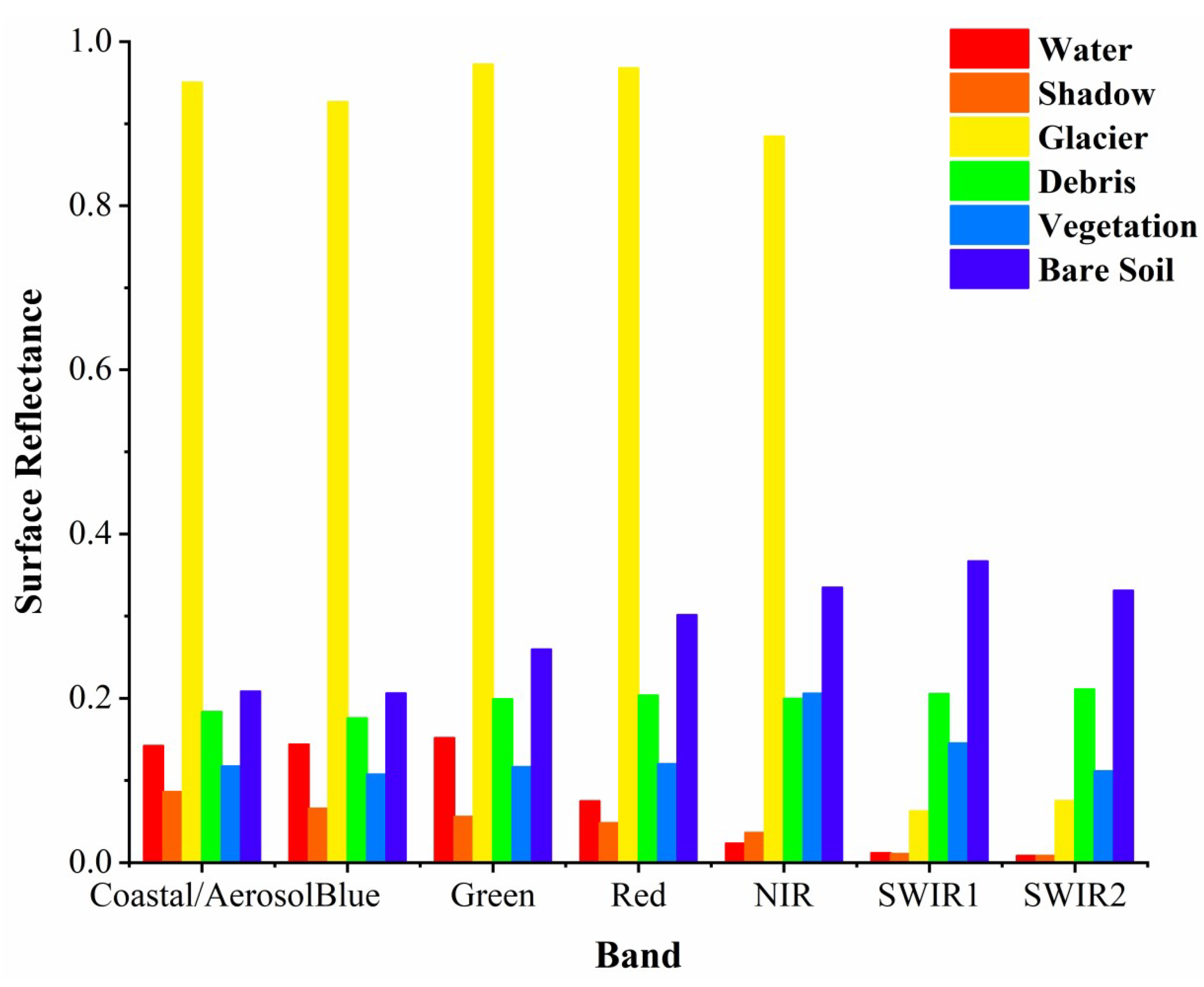
3.2. Analysis Features
We analysed the average surface reflectivity of different surface cover samples (Figure 2) and studied the spectral characteristics of different types of surface cover. It can be seen that the reflectance information of the glacier, debris-covered glaciers and land cover overlap with each other. Vegetation has high reflectance in the near-infrared band and low reflectance in the red band. NDVI can distinguish vegetation cover with high NDVI value from other land cover types with low or negative NDVI value. In the same way, useful information can be obtained from the NDWI features of water bodies. The first and second blue bands of Landsat-8 OLI image data have a high degree of recognition for the glaciers in the shadow area [62], which are the dominant band, and this helps distinguish glacier information in the shadow area. Snow-ice has high spectral reflectance in the visible spectrum (VIS) but low reflectance in the short-wave infrared (SWIR) band [63,64]. Based on the significant difference between the glacial spectral reflectance in the VIS and SWIR bands, snow and ice are identified by thresholding NDSI features. This indicates that using the reflectance information for each class may make it slightly possible to distinguish the classes. Therefore, extraction of some other useful feature information is also necessary.
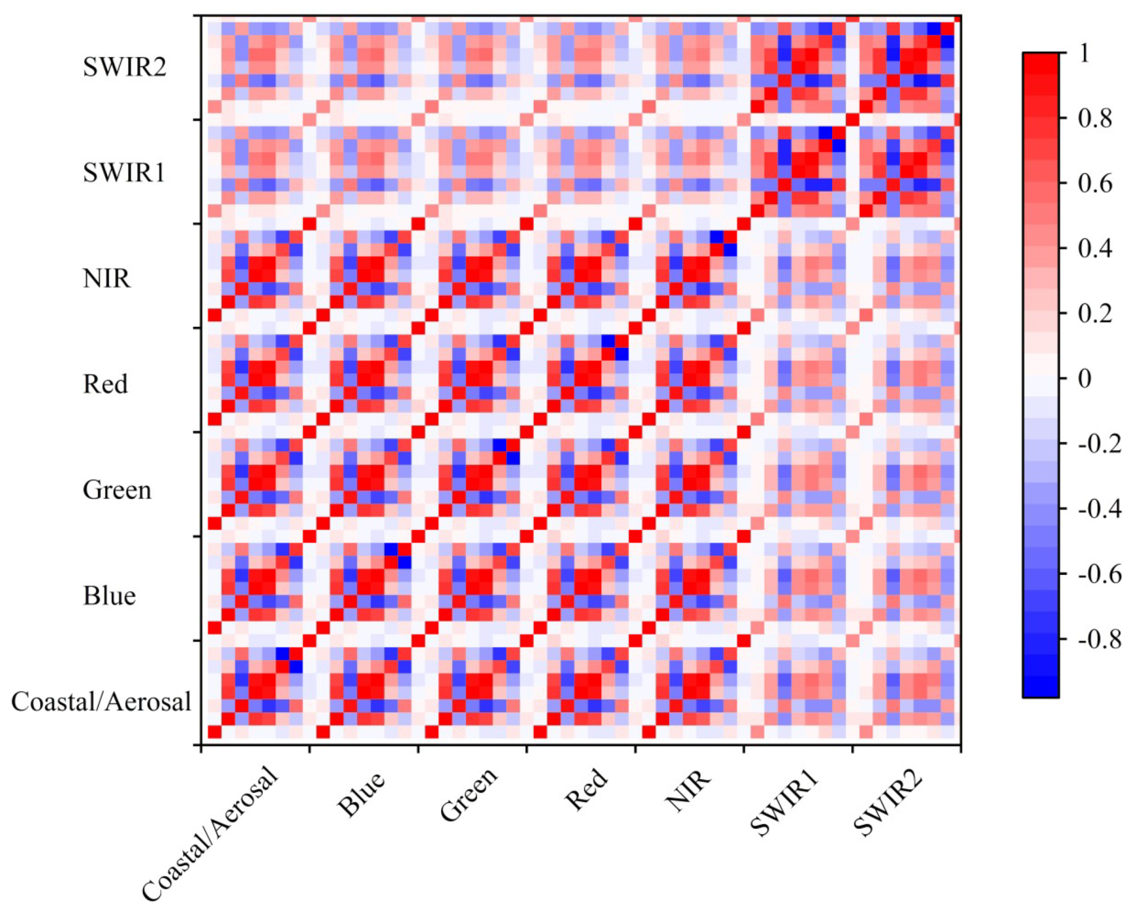
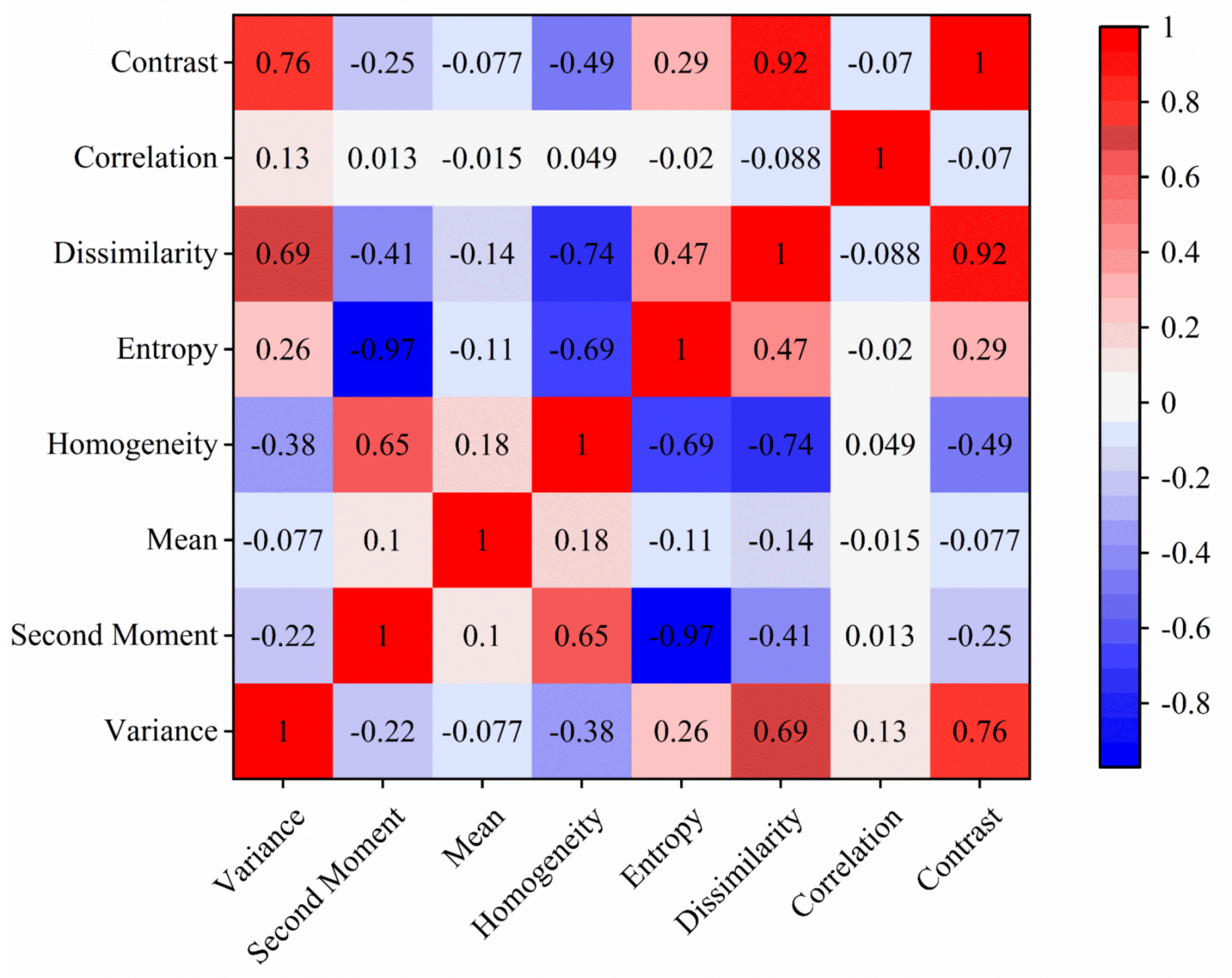
When analysing the texture features in more detail, combined with the correlation coefficient matrix of the spectral index (Figure 3), we noticed that the visible spectrum (VIS) of texture features was more suitable for describing the characteristics of the glacier surface. In addition, the correlation analysis between the 8 texture features was performed to obtain the correlation coefficient (Figure 4). There is a consistent correlation between the mean and other texture features, which plays a decisive role in the mapping of glaciers. Since variance, homogeneity, contrast, and dissimilarity are all texture features that measure pixel deviation, the correlation between the four features is relatively high, and these features can play an auxiliary role in the classification of glaciers. The combination of three texture features of entropy, second moment and correlation makes it difficult to distinguish glaciers from other area classes.
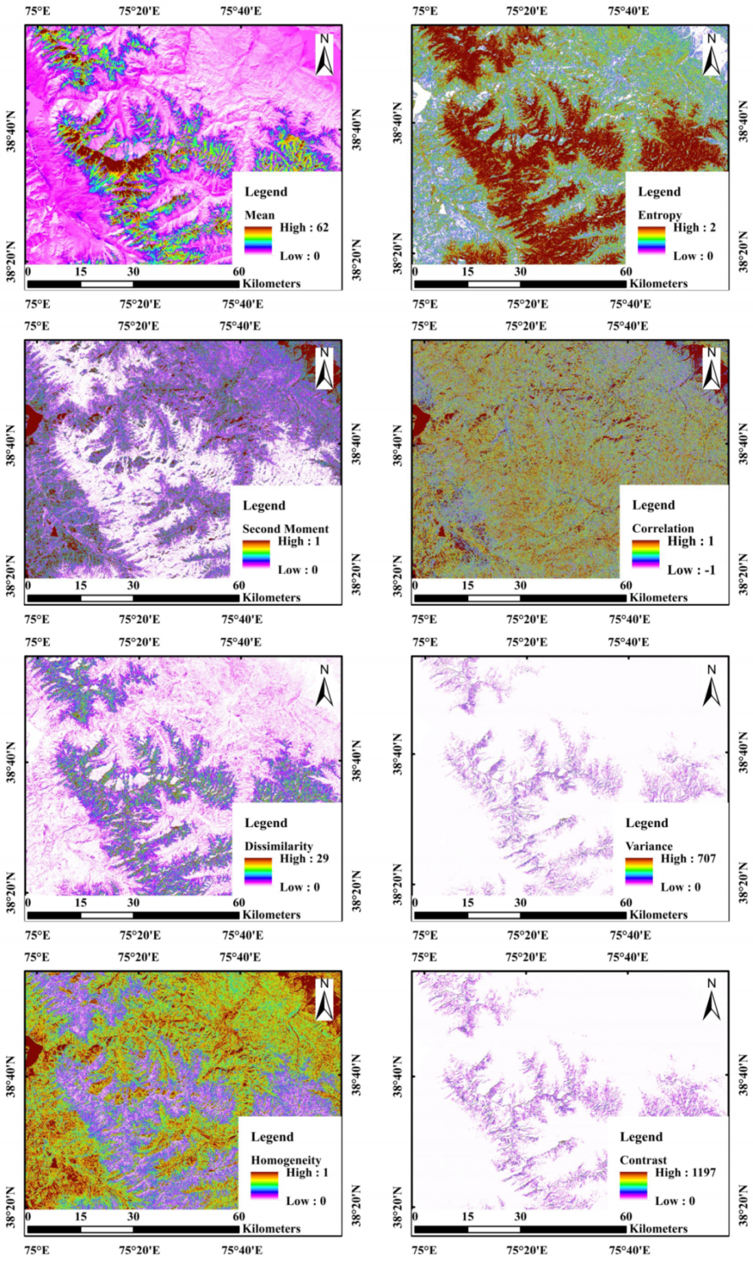
Examples of texture features for the Random Forest classification method for a portion of the study area in ArcGIS shown that the general outline of the glacier was visible on the mean feature image, but, in other texture features, identification of glacier areas was not distinct (Figure 5).
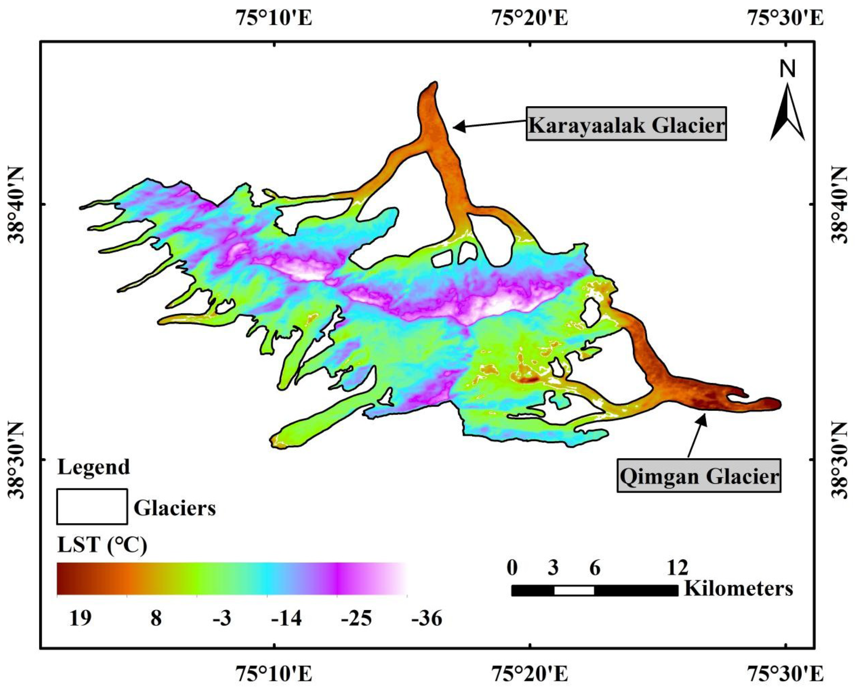
Since the debris had similar spectral characteristics to the surrounding bare land, it was very difficult to decide or classify based on surface reflectance only [65]. The difference in LST between the debris and surrounding terrain is helpful to distinguish as debris-covered glaciers always have lower temperature than the surrounding bare land. To show the difference of LST in comparison with glaciers and debris-covered glaciers, we demonstrated this difference using the LST map shown in Figure 6. The brown area represented the LST of the debris-covered glaciers, typically Karayaalak glacier and Qimgan glacier. The deeper the blue colour, the more sparsely the debris was covered and the green area represented the LST of the clean snow-ice coverage completely. Last but not least, the purple area represented shadow-covered glaciers. We noted that LST retrieved from remote sensing is not the actual surface temperature, but an apparent temperature that makes distinguishing different surface types easier. Therefore, with the support of the LST information map, glaciers and debris-covered glaciers can be differentiated.
In summary, these features are very supportive to determine glaciers, debris-covered glaciers, and other area classes. Thus, the spectral, textural, temperature, topographic and movement velocity features were combined into a final 81-layer superposition that was exploited as the classification input feature of the Random Forest classifier.
4. Random Forest Classification
Random Forest is a combination algorithm, based on a decision tree, proposed by Breiman (2001) [66]. It is an ensemble learning algorithm that is carried out in sample space and feature space at the same time [32,45]. Immediately, each decision tree in the forest relies on a random vector composed of parameters determined by training. Each tree generates an independent and identically distributed training sample set through the Bagging algorithm and uses these sample sets for training while selecting some features in the feature set to construct the decision tree [30,67]. Random has two meanings. One is to randomly select data as training samples with replacement in the training data, and the other is to randomly select the part of the features to construct the model when building a decision tree model. This reduces the correlation between the constructed decision trees, thereby improving the accuracy of the model. The Random Forest algorithm performs better on large data sets and can be used to process high-dimensional data [31,32]. At the same time, it can adapt to various types of data and has high accuracy in complex and large-scale data setting degrees. Furthermore, in the entire algorithm implementation process, random feature selection is introduced to enhance the feature extraction ability, which can often screen out the most important features, have a certain degree of anti-noise ability, and also avoid overfitting problems to a certain extent.
Random Forest is an ensemble learning method that integrates decision trees through bagging [29,68]. In this paper, a Random Forest model is constructed through the machine learning platform Scikit-Learn (http://scikit-learn.org, 2018). By adjusting the parameters of the Random Forest Classifier in Scikit-Learn, the specific structure of the constructed Random Forest is adjusted. The parameters can be divided into bagging integration method parameters and decision tree parameters [30,67], according to the experimental plan of this research; through a large number of experiments, it is found that the specific parameter settings are those shown in Table 3.
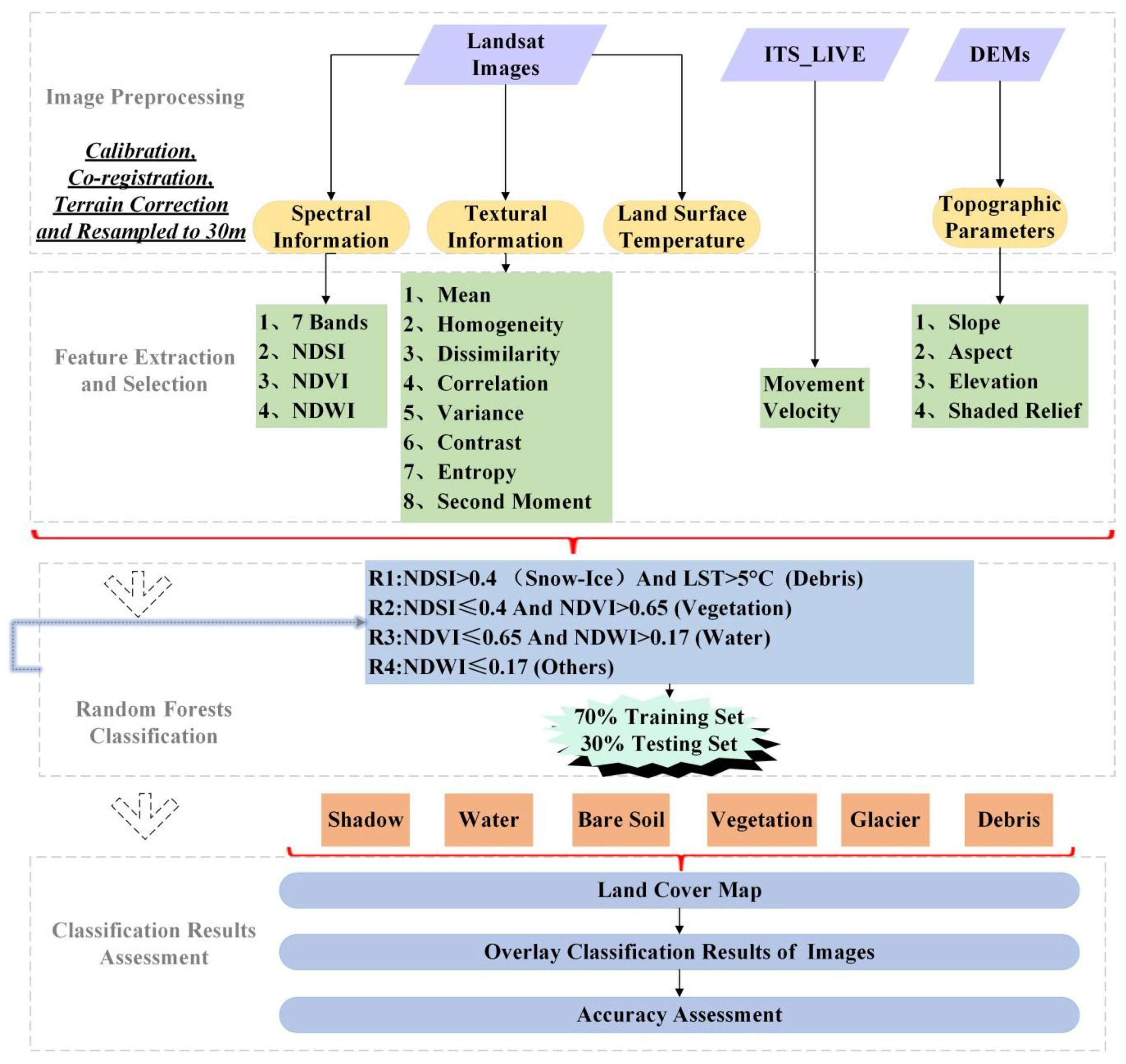
Considering the information mentioned above, the NDSI, NDVI, NDWI and LST images were used as inputs to perform rule-based image segmentation of satellite images. Generally, the determination of the rule-based segmentation depends on the characteristics of the study area; NDVI ranges from 0.65 to 1.0, representing dense vegetation or tropical rainforest. Vegetation has much smaller values, which enable easy distinguishing between vegetation from water bodies. NDSI results confirmed the threshold of 0.4, widely used in the literature, as ideal for mapping snow. When the threshold of NDSI is between 0.25–0.45, it can effectively distinguish between snow and non-snow. Another important consideration is LST. We assumed that most of the glaciers, particularly debris-covered parts, have experienced a significant change in surface land temperature. Other features are used as auxiliary parameters. The specific rules are shown in the workflow of the Random Forest Classifier Model (Figure 7).
In this study, the classification scheme considered six major land cover types: snow, mixed ice (glacier), supraglacial debris and debris (debris), bare soil, water bodies, vegetation, and shadow (shadowed ice and terrain shadows). We used the shadow as a category because the glaciers in the research area were mainly distributed in high valleys and undulating mountainous areas. A glacier situated in the shadow of a mountain was easily covered by the shadow of the mountain in the image. The area of the glaciers covered by the shadow on the image could not be ignored [69]. A flowchart of this study is illustrated in Figure 7. There are two main steps: firstly, we need to extract training features, mainly spectral, texture and temperature features extracted from Landsat images; elevation and topographic features extracted from DEMs; and movement velocity feature extracted from ITS_LIVE. Secondly, it is necessary to combine all these features into a 1 × N-dimensional vector of each pixel, and train and test the Random Forest classifier to generate classification maps for each category (glaciers, debris-covered glaciers, and others). The most important is that a region-based accuracy evaluation is performed by comparing the classification results with reference data to evaluate the performance of the proposed method of the Random Forest classifier.
4.1. Selection of Classification Samples
We only used the images collected on 20 October 2017 for classification, sample selection and training the Random Forest classifier; we used Google Earth high spatial resolution images to visually interpret Landsat-8 images and collected and classified samples of six land cover types (Figure 8). In the Random Forest algorithm [30,67,70], each iteration will generate a sample subset. Nearly 33% of the samples in the entire sample will not appear in each sample subset and these data are called Out-Of-Bag (OOB) data. OOB data can be used to estimate the generalization error of a combined classifier or to estimate the importance of individual features. To obtain the Random Forest’s OOB data misclassification rate, it is necessary to count the classification results of these trees for the sample, and calculate the proportion of the number of misclassified samples to the total number of samples [29,68]. Breiman (2001) [66] proved that the OOB data misclassification rate is an unbiased estimate of the Random Forest generalization error. More specifically, 70% of the random samples were utilised for training and the remaining 30% were utilised for testing to evaluate the classification results.
4.2. Selection of Experimental Scheme
Five characteristic variables were used in the study area, including spectral, texture, temperature, topographic and glacier movement velocity features. Three different combination test schemes were constructed for the above characteristic variables. Random Forest was used to screen out the best combination information suitable for glacier classification (Table 4).
5. Results
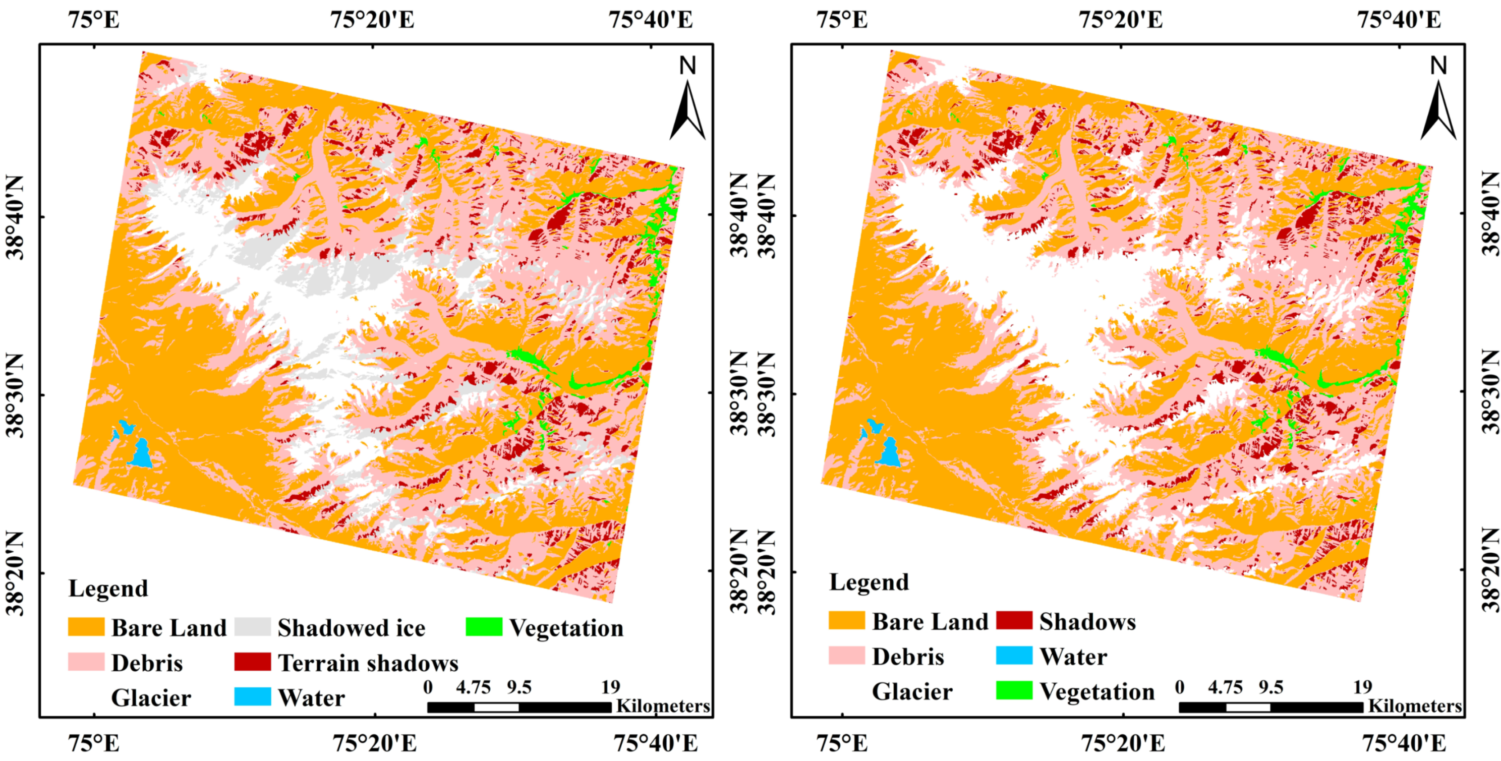
When using images for classification, there were still some incorrectly classified areas, and these pixels needed to be deleted in post-processing; therefore, we used the spatial analysis tool in ArcGIS 10.2 to manually reclassify the incorrectly classified areas. We reclassified shadowed ice to glaciers and subsequently obtained the final glacier classification map. Then, the final glacier classification map was obtained. Preliminary classification results based on the Landsat-8 image acquired on 20 October 2017 (Figure 9) illustrated that when used for classification, Random Forest can provide the spatial distribution of the glaciers’ surface and other land cover types better than traditional algorithms.
5.1. Accuracy Assessment
For pixel-based Random Forest classification, the most common accuracy evaluation indicators, including overall accuracy based on the classification confusion matrix, Kappa coefficient, producer’s accuracy, and user’s accuracy [71], were applied for debris-covered glaciers. Classification results of the three test schemes were compared and classification accuracy is illustrated in Table 5.
Results showed that the overall accuracy of Scheme 1 was the lowest, at 97.42%; those of Schemes 2 and 3 improved by 0.01% and 0.18%, respectively, and the Kappa coefficient increased by 0.0002 and 0.0028, indicating that the addition of topographic feature information and movement velocity features can effectively improve classification accuracy. For the user’s accuracy and producer’s accuracy of a single scheme, topographic features and movement velocity features again proved to be beneficial for improving classification accuracy. Although there were differences in classification accuracy of individual features between different methods, the feature selection method proposed in this study can generally effectively improve the accuracy of glacier classification. The optimal classification result of Scheme 3 is illustrated in Figure 10.
Areas of six types of land cover were estimated by the Random Forest classifier based on the Landsat-8 image acquired on 20 October 2017 (Table 6). The study area was dominated by glaciers (including snow ice, mixed ice, debris, and shadow ice) covering an area of 15.18%.
5.2. Spatial Characteristics of Mountain Glaciers
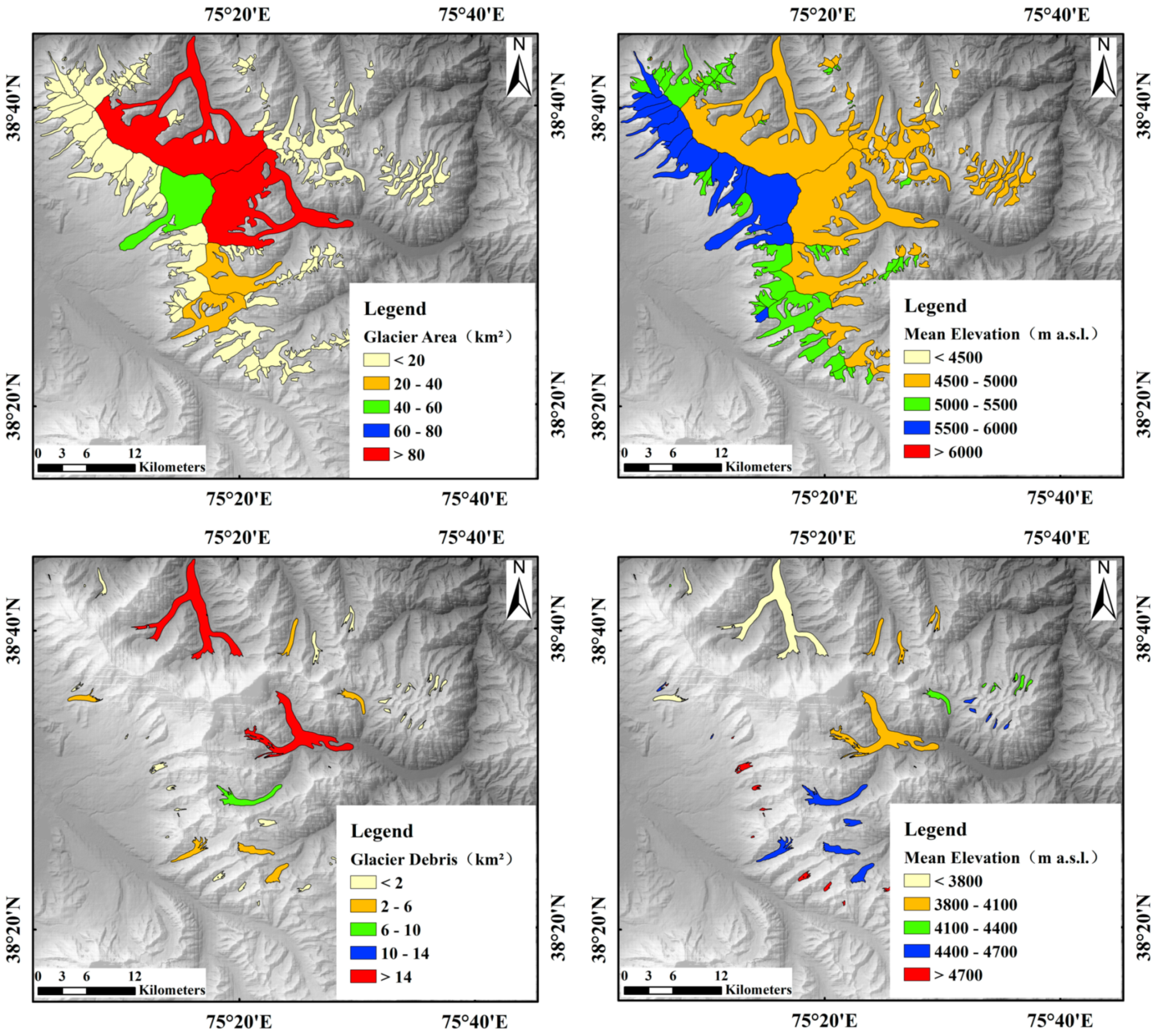
In the study area, the total area occupied by glaciers was 605.117 km2, of which 85.398 km2 were covered by debris and 519.718 km2 were not covered by debris. The altitude at which glaciers occurred varied from 2832 to 7577 m. The glaciers’ area and elevation were divided into five equal parts according to their respective attributes. The spatial distribution of changes in the area of glaciers and debris-covered glaciers is illustrated in Figure 11. The area and elevation distribution of glaciers show typical patterns of mountain glaciers. The mean elevation of glaciers in different areas indicates that the distribution of small glaciers is higher than that of large glaciers. Figure 11 also illuminated that clean glaciers are generally distributed at a higher elevation than debris-covered glaciers. All glaciers larger than 80 km2 are covered by debris, which indicates that there is a higher possibility of debris cover on large glaciers. The results of this study are consistent with previous observations [17,72].
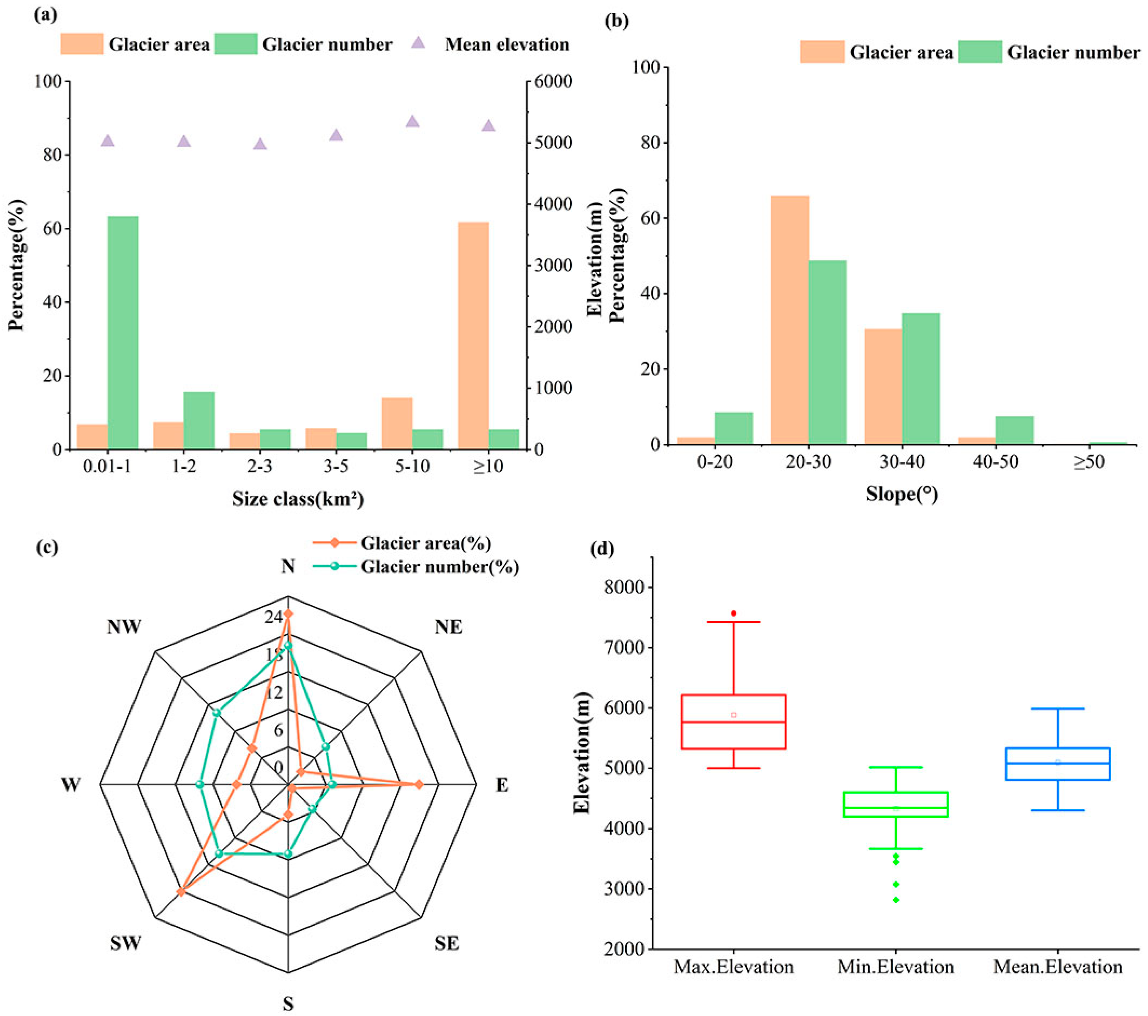
There was a strongly asymmetrical pattern in the number and total area of small glaciers (<1 km2) and large glaciers (≥10 km2). Although small glaciers accounted for 63.32% of the total area occupied by glaciers, these only accounted for 6.83% of the total glacial area in the study area and this finding was consistent with the characteristics of glaciers in mid-latitude mountains. The largest glacial area contained only 11 glaciers larger than 10 km2 in size, accounting for 61.69% of the total glacial area. The mean elevation of different glaciers showed that the elevation of small glaciers was lower than that of large glaciers (Figure 12a). The distribution number and area of glaciers according to the glacier mean slope (Figure 12b) illustrated that the glacial slope from 20° to 35° accounted for a large part of the total area. Only a few glaciers had slopes with a total of less than 20° or more than 50°. In terms of the number of glaciers present, ice bodies were mainly oriented north: 44 ice bodies faced north and 117 flowed in a northeasterly direction, and 28 glaciers faced northwest (Figure 12c). A total of 61% of the glaciated surface area faced north. The spatial distribution of the glaciers revealed that the location of glaciers was mainly affected by local topography. Figure 12d illustrates that the elevation of the eastern Pamir glacier in the study area fluctuated greatly, with the average altitude being 5040 m, the lowest altitude 4608 m, and the highest altitude 5482 m.
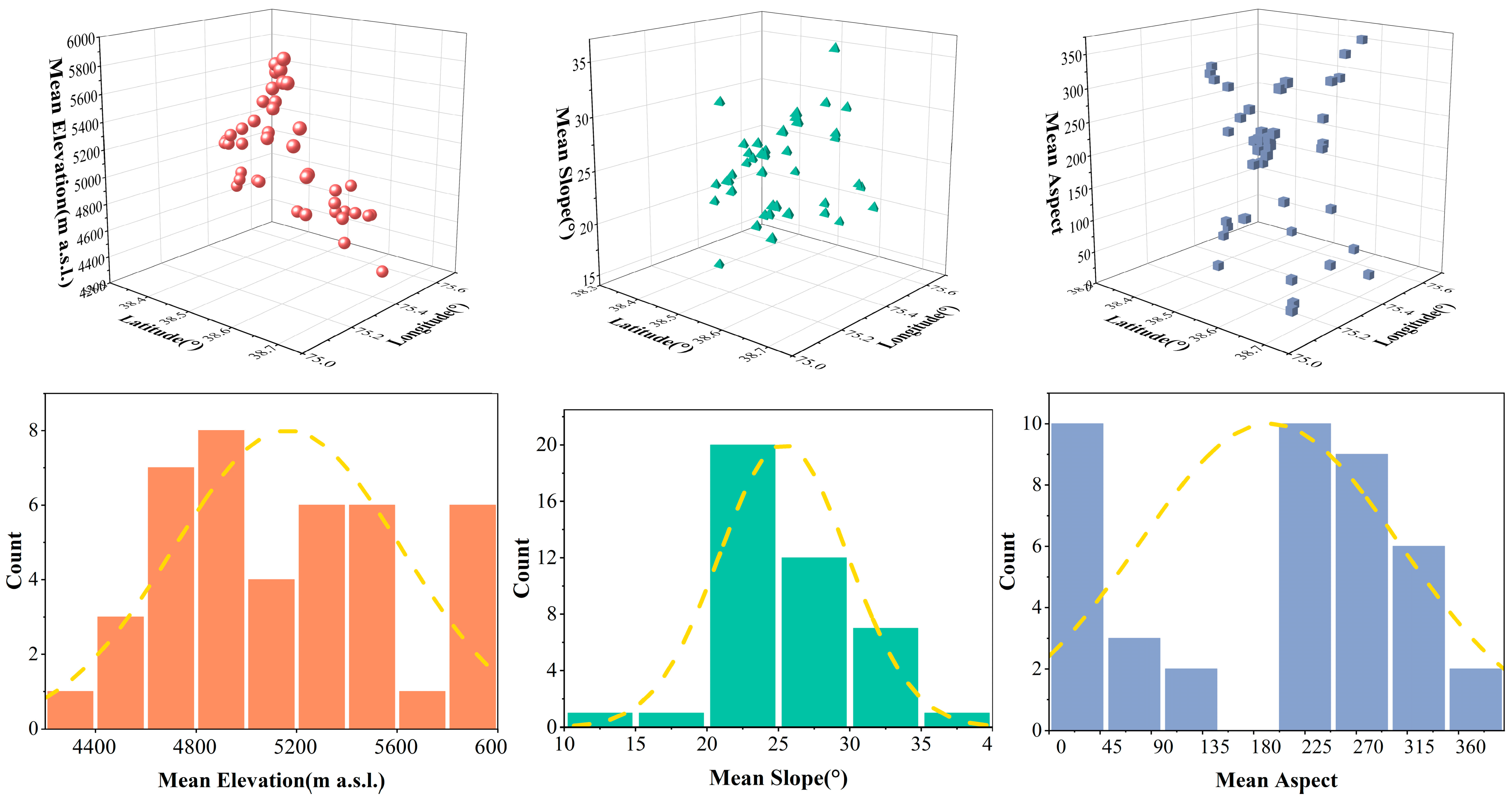
The elevation, slope, and aspect of the glacier were combined with the geographic location, and then the number of glaciers in each category were counted (Figure 13). The analysis shows that the glaciers in the study area are mainly distributed between 38.4° and 38.7° N, and between 75.0° and 75.6° E. The distribution of glaciers is uneven with the increasing elevation, and the distribution of glaciers is denser in high and low elevation areas; meanwhile, the slope of glaciers in the study area is mainly concentrated between 20° and 35°. Along with the increase in the latitude and longitude, slope and aspect both have the tendency of ascension, which symbolizes the steep mountains in the study area and demonstrates good geographical conditions for the development of glaciers.
The climate was dry and cold, and humid monsoon air in the west and southwest was intercepted by high mountains in the study area, providing an ideal physical and geographical basis for the accumulation of glaciers. These conditions were consistent with our observation that the altitude of the glaciers in this area varied from 2832 to 7577 m (Figure 14a). According to DEM data, the glacial elevation map was reclassified into 11 elevation gradients at 500 m intervals. Hypsometry of debris-covered glaciers, non-debris-covered glaciers and total glaciers area based on the mean elevation on the eastern Pamir is illustrated in Figure 14b. During the hypsometrical analysis, the glacial area was 353.053 km2 (58.34% of the total glacial area) at 4500 to 5000 m, 112.223 km2 (18.55% of the total area of the glaciers) at 5000 to 5500 m, and 135.715 km2 (22.43% of the total area of the glaciers) at 5500 to 6000 m.
6. Discussion
6.1. Uncertainties and Limitations in Mapping Glacier Outlines
Samples. Classification samples of the study area were mainly based on Landsat-8 data, but, at a resolution of 30 m, the boundaries of some small features (only a few pixels) were indistinct and difficult to identify. This problem could be partially avoided through the achievement of higher-resolution remote sensing images (GaoFen series or Sentinel series data). Detailed information regarding glacial surface and classification samples covering the entire area is needed to improve the accuracy of Random Forest classification results.
DEM. DEM accuracy was another key factor in this study that directly affected the topographical features of glaciers in the Random Forest classification process. The surface of the glacier and the surrounding environment presented a complex pattern. The 30 m resolution DEM might not have reflected key surface features. ASTER GDEM V2 global digital elevation data were acquired in 2009 and officially released on 6 January 2015. There was a time difference between the acquisition time of the Landsat-8 image selected in this experiment and the release of ASTER GDEM, although there were no obvious elevation changes in the eastern Pamir during the periods. However, it is necessary to match the time scale with experimental data.
Debris cover. Although the thermal infrared bands of optical images can be used to identify debris-covered glaciers [73], the extraction method of thermal infrared bands is based on the assumption that the edge of the glacier has a higher temperature than the inside of the glacier, which is not applicable for the Qinghai–Tibet Plateau, which has thicker debris coverage [74]; more manual correction is needed to get a more accurate glacier boundary. Detailed field surveys could help identify pixels as debris-covered glaciers or other types of land cover. Collecting large quantities of ground data could further improve understanding of glaciers in the region.
Seasonal snow. The high spatial resolution Google Earth images from the study area were generally acquired in winter, therefore thicker snow cover increased the difficulty of accurately identifying glaciers and debris. Seasonal snow, however, impacted on the result, as it should be excluded in a glacier inventory but is difficult to distinguish from glaciers in topographic depressions that can be included [75]. In this research, seasonal snow is detected by comparing multiple Landsat images acquired during the ablation season [52].
Shadows. For glaciers in the alpine region, remote sensing images usually have a large area of mountain shadows. The shadow causes the amount of information reflected by the ground object to be lost or interfered, and the DN value is low in the remote sensing image data, which is difficult to interpret (Figure 2). Failure to identify glaciers in the shadows can lead to incorrect estimates of the glacier area. Supervised and unsupervised classification methods cannot effectively identify glaciers in the shadows [62]. The segmentation thresholds of the conventional ratio method and snow cover index method are not intuitive enough. It is still a difficult task to identify glaciers in shadow areas of large-scale glacier extraction located in in alpine regions.
Cloud coverage. Although the effect of low cloud cover was deliberately selected as the first choice in the initial selection of images, clouds that existed in the study area were not excluded in the experiment. Cloud cover was not regarded as a category in this classification system. The emissivity and shadow caused by cloud cover would also affect the classification results to a certain extent. Special attention should be paid to cloud analysis in future research.
Others. Rule-based image segmentation technology did not detect a small number of glaciers (missing errors). Since the result of the rule-based image segmentation technique is used as the region for extracting the new predictor data set of Random Forest, the error will be propagated to the result. Namely, those glaciers not detected by the former method are not part of the latter’s observations.
Considering all these possibilities, it is obvious from our results that the feature dataset we chose and the threshold used are very suitable for mapping glaciers in high mountain regions.
6.2. Comparison with Previous Glacier Classification Methods and Glacier Inventories
Automatic classification results of Random Forest were compared with three existing glacier inventory datasets: The second glacier inventory dataset of China (CGI2), the Tibetan Plateau glacier data-TPG2017 (TPG2017) and the Glacier inventory of the Pamir and Karakoram (CCI) [23]. CGI2 was based on Landsat TM/ETM+ and ASTER remote sensing images after 2004, regarding CGI and other documents, and included technical links such as image correction, automatic interpretation, field surveys, manual revisions, interactive inspections, and result verifications. TPG2017 was based on Landsat satellite images from three periods and took the uncertainty caused by the limited span of each period into account. Under the guidance of SRTM DEM v4.1 and Google Earth images, the glacier contours (TPG1976, TPG2001 and TPG2013) were manually digitised. To achieve complete multi-time coverage in a reasonable time, only ice cubes without debris were depicted. CCI utilised 28 Landsat TM and ETM + scenes acquired in 2000 to arrive at a homogeneous inventory of the Pamirs and Karakoram Mountains. CCI applied standardised methods and utilised coherent images from advanced land observation satellites to perform automatic digital mapping and manual correction of digital glaciers. These three types of data were obtained by the human–computer interaction method of comprehensive expert experience and knowledge.
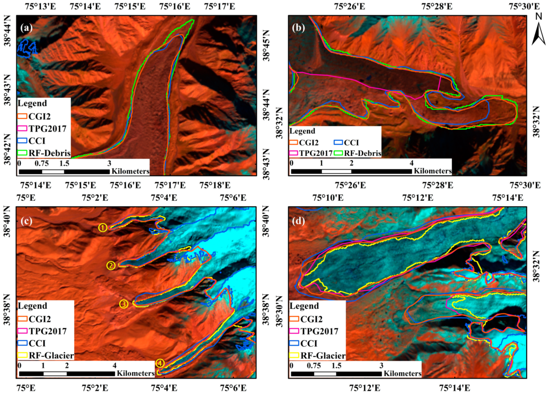
A comparison between the results of the Random Forest classification and the other three glacier datasets is illustrated in Figure 15. Some differences in glacier regions are more likely to be caused by changes in glaciers. Our total glacier area was about 5.7% larger than that of the CGI2. Our results showed that the edge of the debris-covered glaciers was slightly larger than inventories mentioned above (Figure 15a,b) and these debris-covered glaciers are mainly distributed in areas with lower elevations. There are more small glaciers in the middle and high-altitude areas than the low altitude areas. The boundaries of these glaciers (G075083E38637N; G075085E38663E; G075102E38655N and G075116E38641N) (Figure 15c) are consistent with CGI2 and TPG2017. Since there are many debris-covered glaciers in the Qinghai–Tibet Plateau, TPG2017 has not yet drawn a complete glacier map. We compared the glacier boundary drawn by TPG2017 with results obtained by Random Forest and noted that there was no distinct difference between the TPG2017 and CGI2 datasets on most glacier boundaries, or these were identical but there were still significant differences. In the Qimgan Glacier, boundary data of Figure 15b demonstrated that Random Forest results are closer to CGI2, but there was no Nan Qimgan Glacier in TPG2017, mainly because this was classified as debris and not considered a glacier. The boundary between the CCI and CGI2 datasets in the study area fitted perfectly and only a small part of the difference in the outline of the boundary could be due to seasonal ice and snow caused by the difference in the acquisition time of the images. The inconsistency of CGI2, TPG2017 and CCI (Figure 15d) may be due to seasonal snow cover or glacial retreat in the area, as had also been mentioned in other studies [76].
Although the Landsat image was obtained at the end of the ablation season, the classification result of Random Forest depended entirely on the selected remote sensing image. We considered the impact of seasonal snowfall on glacier recognition. Therefore, the use of a single image may not be the best choice for describing the outline of a glacier. Using multi-time images would be a more effective method of minimising the influence of seasonal snow on the extracted glacier contours.
The accuracy of Random Forest is similar to (or even better than) other studies [33,42,43]. The glacier movement provided important information for understanding glacial changes. The velocity of glacier movement was related to slope, aspect, and debris. We introduced the feature of movement velocity to identify glaciers with the help of Random Forest classification and favourable results were obtained. In contrast, obstacles to the recognition of some debris areas remain, Random Forest classification results of the five types of features entered in this study identified glaciers in the clean ice area and this was consistent with the glacier contours of inventories mentioned (Figure 15). All uncertainty values must be viewed from the perspective of method uncertainty, such as including possible snow cover at high altitudes that can easily increase the existence of small glaciers. Excluding these factors, the uncertainty given above is usually much smaller.
In summary, the proposed method is highly robust to all forms of interference and challenging factors encountered in the process of glacier mapping. The outline of the glaciers shows good consistency with the previous datasets, and this method may solve the current inconsistency between the entire glacier inventory datasets.
7. Conclusions
The outline of debris-covered glaciers varies amongst the scientific literature. In this research, we proposed a Random Forest algorithm for debris-covered glaciers’ mapping that automatically minify limitations of traditional monitoring such as mountain and cloud shadows, cloud cover, seasonal snow cover, and debris. The method consists of rule-based image segmentation and the Random Forest classifier model. Rule-based technology extracts discrete objects of interest from Landsat-8 images. The predictive indicators are NDSI, NDWI, NDVI and LST. Then, according to the trained model, glaciers, debris-covered glaciers, and non-glaciers are predicted. The method was tested in the eastern Pamir and demonstrated that the potential of the Random Forest method has high robustness in all glaciers of the eastern Pamir. The proposed method can potentially be used for glacier mapping in other alpine regions.
The proposed machine learning classification method allowed accurate and relatively rapid mapping of debris-covered glaciers while having the advantage of being transferable to other areas and datasets. More importantly, the combination of movement velocity characteristics and the Random Forest algorithm can promote the progress of debris-covered glaciers’ mapping work to a certain extent. Therefore, the methods introduced in this study can fill data gaps in areas with a lack of historical (and/or current) glacier mapping.
In the absence of an appropriate ground truth reference dataset, we used various methods for uncertainty assessment and compared our profile with previous inventories covering the same area. The use of statistics showed that using the rule-based image segmentation and Random Forest algorithm to extract the glacier and automatically map the glacier surface is feasible. Compared with previous inventories, this new inventory, developed by machine learning algorithm, will benefit future glacier studies and provide technical support for rapid glacier inventory.
Although there is no cloud in the glacier area we chose, what can not be ignored is the consideration of clouds, in order to better promote the method adopted in this article. The extraction accuracy of debris-covered glaciers using SAR interference coefficients is significantly better than that of optical images, owing to the ability to penetrate clouds and fog. Moreover, we hope to use higher resolution multi-source satellite data based on fully automated machine learning methods to extract glacier features. It can be expected that this will greatly reduce the manpower required and will help improve the classification accuracy for mapping debris-covered glaciers.
Author Contributions
Conceptualization, Z.Z.; methodology, Y.L.; validation, Y.L.; resources, Y.L. and D.H.; writing—original draft preparation, Y.L. and Z.Z.; writing—review and editing, Y.L. and Z.Z.; visualization, Y.L. All authors have read and agreed to the published version of the manuscript.
Funding
This research was funded by the National Natural Science Foundation of China (Grant Nos. 41701087 and 42071085).
Acknowledgments
The authors would like to thank the Geospatial Data Cloud site (http://www.gscloud.cn) for the ASTER GDEM V2 data and the Landsat-8 images, NASA’s MEaSUREs project (https://its-live.jpl.nasa.gov/) for the Inter-mission Time Series of Land Ice Velocity and Elevation (ITS_LIVE), the National Tibetan Plateau Data Center (http://data.tpdc.ac.cn) for the second glacier inventory dataset of China (version 1.0) (2006–2011) and the Tibetan Plateau glacier data—TPG2017 (v1.0). We are grateful to Mölg (2018): Glacier inventory of Pamir and Karakoram, and for the link to GIS files. (https://doi.pangaea.de/10.1594/PANGAEA.894707).
Conflicts of Interest
The authors declare no conflict of interest.
References
- Immerzeel, W.W.; Van Beek, L.P.H.; Bierkens, M.F.P. Climate Change Will Affect the Asian Water Towers. Science 2010, 328, 1382–1385. [Google Scholar]
- Gardner, A.S.; Moholdt, G.; Cogley, J.G.; Wouters, B.; Arendt, A.A.; Wahr, J.; Berthier, E.; Hock, R.; Pfeffer, W.T.; Kaser, G.; et al. A Reconciled Estimate of Glacier Contributions to Sea Level Rise: 2003 to 2009. Science 2013, 340, 852–857. [Google Scholar] [CrossRef] [PubMed] [Green Version]
- Andreas, K.; Etienne, B.; Christopher, N.; Julie, G.; Yves, A. Contrasting patterns of early twenty-first-century glacier mass change in the Himalayas. Nature 2012, 488, 495–498. [Google Scholar]
- Kääb, A.; Treichler, D.; Nuth, C.; Berthier, E. Brief Communication: Contending estimates of 2003–2008 glacier mass balance over the Pamir–Karakoram–Himalaya. Cryosphere 2015, 9, 557–564. [Google Scholar] [CrossRef] [Green Version]
- Lamsal, D.; Sawagaki, T.; Watanabe, T.; Byers, A.C. Assessment of glacial lake development and prospects of outburst susceptibility: Chamlang South Glacier, eastern Nepal Himalaya. Geomat. Nat. Hazards Risk 2016, 7, 403–423. [Google Scholar] [CrossRef] [Green Version]
- Zhao, L.; Ding, R.; Moore, J.C. The High Mountain Asia glacier contribution to sea-level rise from 2000 to 2050. Ann. Glaciol. 2016, 57, 223–231. [Google Scholar] [CrossRef] [Green Version]
- Kraaijenbrink, P.D.A.; Shea, J.M.; Pellicciotti, F.; de Jong, S.M.; Immerzeel, W.W. Object-based analysis of unmanned aerial vehicle imagery to map and characterise surface features on a debris-covered glacier. Remote Sens. Environ. 2016, 186, 581–595. [Google Scholar] [CrossRef]
- Kääb, A.; Bolch, T.; Casey, K.; Heid, T.; Kargel, J.S.; Leonard, G.J.; Paul, F.; Raup, B.H. Glacier Mapping and Monitoring Using Multispectral Data. In Global Land Ice Measurements from Space; Kargel, J.S., Leonard, G.J., Bishop, M.P., Kääb, A., Raup, B.H., Eds.; Springer Praxis Books; Springer: Berlin/Heidelberg, Germany, 2014; pp. 75–112. ISBN 978-3-540-79818-7. [Google Scholar]
- Williams, R.S.; Hall, D.K.; Sigurðsson, O.; Chien, J.Y.L. Comparison of satellite-derived with ground-based measurements of the fluctuations of the margins of Vatnajökull, Iceland, 1973–92. Ann. Glaciol. 1997, 24, 72–80. [Google Scholar] [CrossRef]
- Burns, P.; Nolin, A. Using atmospherically-corrected Landsat imagery to measure glacier area change in the Cordillera Blanca, Peru from 1987 to 2010. Remote Sens. Environ. 2014, 140, 165–178. [Google Scholar] [CrossRef] [Green Version]
- Singh, D.K.; Thakur, P.K.; Naithani, B.P.; Kaushik, S. Quantifying the sensitivity of band ratio methods for clean glacier ice mapping. Spat. Inf. Res. 2020. [Google Scholar] [CrossRef]
- Pope, A.; Rees, W.G. Impact of spatial, spectral, and radiometric properties of multispectral imagers on glacier surface classification. Remote Sens. Environ. 2014, 141, 1–13. [Google Scholar] [CrossRef]
- Gjermundsen, E.F.; Mathieu, R.; Kääb, A.; Chinn, T.; Fitzharris, B.; Hagen, J.O. Assessment of multispectral glacier mapping methods and derivation of glacier area changes, 1978–2002, in the central Southern Alps, New Zealand, from ASTER satellite data, field survey and existing inventory data. J. Glaciol. 2011, 57, 667–683. [Google Scholar] [CrossRef] [Green Version]
- Paul, F. Changes in glacier area in Tyrol, Austria, between 1969 and 1992 derived from Landsat 5 Thematic Mapper and Austrian Glacier Inventory data. Int. J. Remote Sens. 2002, 23, 787–799. [Google Scholar] [CrossRef]
- Guo, W.; Liu, S.; Xu, J.; Wu, L.; Shangguan, D.; Yao, X.; Wei, J.; Bao, W.; Yu, P.; Liu, Q.; et al. The second Chinese glacier inventory: Data, methods and results. J. Glaciol. 2015, 61, 357–372. [Google Scholar] [CrossRef] [Green Version]
- Liu, S.; Yao, X.; Guo, W.; Xu, J.; Shangguan, D.; Wei, J.; Bao, W.; Wu, L. The contemporary glaciers in China based on the Second Chinese Glacier Inventory. Acta Geogr. Sin. 2015, 70, 3–16. [Google Scholar] [CrossRef]
- Paul, F.; Huggel, C.; Kääb, A. Combining satellite multispectral image data and a digital elevation model for mapping debris-covered glaciers. Remote Sens. Environ. 2004, 89, 510–518. [Google Scholar] [CrossRef]
- Winsvold, S.H.; Kääb, A.; Nuth, C.; Andreassen, L.M.; van Pelt, W.J.J.; Schellenberger, T. Using SAR satellite data time series for regional glacier mapping. Cryosphere 2018, 12, 867–890. [Google Scholar] [CrossRef] [Green Version]
- Karimi, N.; Farokhnia, A.; Karimi, L.; Eftekhari, M.; Ghalkhani, H. Combining optical and thermal remote sensing data for mapping debris-covered glaciers (Alamkouh Glaciers, Iran). Cold Reg. Sci. Technol. 2012, 71, 73–83. [Google Scholar] [CrossRef]
- Wang, X.; Gao, X.; Zhang, X.; Wang, W.; Yang, F. An Automated Method for Surface Ice/Snow Mapping Based on Objects and Pixels from Landsat Imagery in a Mountainous Region. Remote Sens. 2020, 12, 485. [Google Scholar] [CrossRef] [Green Version]
- Bolch, T. Climate change and glacier retreat in northern Tien Shan (Kazakhstan/Kyrgyzstan) using remote sensing data. Glob. Planet. Chang. 2007, 56, 1–12. [Google Scholar] [CrossRef]
- Wang, P.; Li, Z.; Li, H.; Zhang, Z.; Xu, L.; Yue, X. Glaciers in Xinjiang, China: Past Changes and Current Status. Water 2020, 12, 2367. [Google Scholar] [CrossRef]
- Mölg, N.; Bolch, T.; Rastner, P.; Strozzi, T.; Paul, F. A consistent glacier inventory for Karakoram and Pamir derived from Landsat data: Distribution of debris cover and mapping challenges. Earth Syst. Sci. Data 2018, 10, 1807–1827. [Google Scholar] [CrossRef] [Green Version]
- Ye, Q.; Zong, J.; Tian, L.; Cogley, J.G.; Song, C.; Guo, W. Glacier changes on the Tibetan Plateau derived from Landsat imagery: Mid-1970s–2000–13. J. Glaciol. 2017, 63, 273–287. [Google Scholar] [CrossRef] [Green Version]
- Azzoni, R.S.; Sarıkaya, M.A.; Fugazza, D. Turkish glacier inventory and classification from high-resolution satellite data. Med. Geosc. Rev. 2020, 2, 153–162. [Google Scholar] [CrossRef]
- Marochov, M.; Carbonneau, P.; Stokes, C. Automated image classification of outlet glaciers in Greenland using deep learning. In Proceedings of the EGU General Assembly Conference Abstracts, Göttingen, Germany, 4–8 May 2020; Volume 22, p. 19996. [Google Scholar]
- Alifu, H.; Vuillaume, J.-F.; Johnson, B.A.; Hirabayashi, Y. Machine-learning classification of debris-covered glaciers using a combination of Sentinel-1/-2 (SAR/optical), Landsat 8 (thermal) and digital elevation data. Geomorphology 2020, 369, 107365. [Google Scholar] [CrossRef]
- Speiser, J.L.; Miller, M.E.; Tooze, J.; Ip, E. A comparison of random forest variable selection methods for classification prediction modeling. Expert Syst. Appl. 2019, 134, 93–101. [Google Scholar] [CrossRef]
- Dong, X.; Yu, Z.; Cao, W.; Shi, Y.; Ma, Q. A survey on ensemble learning. Front. Comput. Sci. 2020, 14, 241–258. [Google Scholar] [CrossRef]
- Hillebrand, E.; Lukas, M.; Wei, W. Bagging weak predictors. Int. J. Forecast. 2020, S0169207020300649. [Google Scholar] [CrossRef]
- Belgiu, M.; Drăguţ, L. Random forest in remote sensing: A review of applications and future directions. ISPRS J. Photogramm. Remote Sens. 2016, 114, 24–31. [Google Scholar] [CrossRef]
- Pal, M. Random forest classifier for remote sensing classification. Int. J. Remote Sens. 2005, 26, 217–222. [Google Scholar] [CrossRef]
- Schoppa, L.; Disse, M.; Bachmair, S. Evaluating the performance of random forest for large-scale flood discharge simulation. J. Hydrol. 2020, 590, 125531. [Google Scholar] [CrossRef]
- Pham, L.T.; Luo, L.; Finley, A.O. Evaluation of Random Forest for short-term daily streamflow forecast in rainfall and snowmelt driven watersheds. Hydrol. Earth Syst. Sci. Discuss. 2020, 1–33. [Google Scholar] [CrossRef]
- Mosavi, A.; Hosseini, F.S.; Choubin, B.; Goodarzi, M.; Dineva, A.A. Groundwater Salinity Susceptibility Mapping Using Classifier Ensemble and Bayesian Machine Learning Models. IEEE Access 2020, 8, 145564–145576. [Google Scholar] [CrossRef]
- Melesse, A.M.; Khosravi, K.; Tiefenbacher, J.P.; Heddam, S.; Kim, S.; Mosavi, A.; Pham, B.T. River Water Salinity Prediction Using Hybrid Machine Learning Models. Water 2020, 12, 2951. [Google Scholar] [CrossRef]
- Band, S.S.; Janizadeh, S.; Pal, S.C.; Chowdhuri, I.; Siabi, Z.; Norouzi, A.; Melesse, A.M.; Shokri, M.; Mosavi, A. Comparative Analysis of Artificial Intelligence Models for Accurate Estimation of Groundwater Nitrate Concentration. Sensors 2020, 20, 5763. [Google Scholar] [CrossRef] [PubMed]
- Mosavi, A.; Golshan, M.; Janizadeh, S.; Choubin, B.; Melesse, A.M.; Dineva, A.A. Ensemble models of GLM, FDA, MARS, and RF for flood and erosion susceptibility mapping: A priority assessment of sub-basins. Geocarto Int. 2020, 1–20. [Google Scholar] [CrossRef]
- Mosavi, A.; Sajedi-Hosseini, F.; Choubin, B.; Taromideh, F.; Rahi, G.; Dineva, A.A. Susceptibility Mapping of Soil Water Erosion Using Machine Learning Models. Water 2020, 12, 1995. [Google Scholar] [CrossRef]
- Choubin, B.; Borji, M.; Hosseini, F.S.; Mosavi, A.; Dineva, A.A. Mass wasting susceptibility assessment of snow avalanches using machine learning models. Sci. Rep. 2020, 10, 18363. [Google Scholar] [CrossRef]
- Mosavi, A.; Shirzadi, A.; Choubin, B.; Taromideh, F.; Hosseini, F.S.; Borji, M.; Shahabi, H.; Salvati, A.; Dineva, A.A. Towards an Ensemble Machine Learning Model of Random Subspace Based Functional Tree Classifier for Snow Avalanche Susceptibility Mapping. IEEE Access 2020, 8, 145968–145983. [Google Scholar] [CrossRef]
- Zhang, J.; Jia, L.; Menenti, M.; Hu, G. Glacier Facies Mapping Using a Machine-Learning Algorithm: The Parlung Zangbo Basin Case Study. Remote Sens. 2019, 11, 452. [Google Scholar] [CrossRef] [Green Version]
- Khan, A.A.; Jamil, A.; Hussain, D.; Taj, M.; Jabeen, G.; Malik, M.K. Machine-Learning Algorithms for Mapping Debris-Covered Glaciers: The Hunza Basin Case Study. IEEE Access 2020, 8, 12725–12734. [Google Scholar] [CrossRef]
- Kaplan, G.; Avdan, U. Monthly Analysis of Wetlands Dynamics Using Remote Sensing Data. ISPRS Int. J. Geoinf. 2018, 7, 411. [Google Scholar] [CrossRef] [Green Version]
- Tian, S.; Zhang, X.; Tian, J.; Sun, Q. Random Forest Classification of Wetland Landcovers from Multi-Sensor Data in the Arid Region of Xinjiang, China. Remote Sens. 2016, 8, 954. [Google Scholar] [CrossRef] [Green Version]
- Wang, L.; Dong, T.; Zhang, G.; Niu, Z. LAI Retrieval using PROSAIL Model and Optimal Angle Combination of Multi-Angular Data in Wheat. IEEE J. Sel. Top. Appl. Earth Obs. Remote Sens. 2013, 6, 1730–1736. [Google Scholar] [CrossRef]
- Wu, K.; Liu, S.; Zhu, Y.; Liu, Q.; Jiang, Z. Dynamics of glacier surface velocity and ice thickness for maritime glaciers in the southeastern Tibetan Plateau. J. Hydrol. 2020, 590, 125527. [Google Scholar] [CrossRef]
- Guo, L.; Li, J.; Li, Z.; Wu, L.; Li, X.; Hu, J.; Li, H.; Li, H.; Miao, Z.; Li, Z. The Surge of the Hispar Glacier, Central Karakoram: SAR 3-D Flow Velocity Time Series and Thickness Changes. J. Geophys. Res. Solid Earth 2020, 125. [Google Scholar] [CrossRef]
- Jiskoot, H.; DeJong, E.; Van Wychen, W.; Cooley, J. The need for global glacier speed to combine measured velocity with balance velocity. In Proceedings of the EGU General Assembly Conference Abstracts, Göttingen, Germany, 4–8 May 2020; Volume 22, p. 12515. [Google Scholar]
- Greene, C.A.; Gardner, A.S.; Andrews, L.C. Detecting seasonal ice dynamics in satellite images. Cryosphere Discuss. 2020, 1–21. [Google Scholar] [CrossRef]
- Shangguan, D.; Liu, S.; Ding, Y.; Guo, W.; Xu, B.; Xu, J.; Jiang, Z. Characterizing the May 2015 Karayaylak Glacier surge in the eastern Pamir Plateau using remote sensing. J. Glaciol. 2016, 62, 944–953. [Google Scholar] [CrossRef] [Green Version]
- Paul, F.; Bolch, T.; Briggs, K.; Kääb, A.; McMillan, M.; McNabb, R.; Nagler, T.; Nuth, C.; Rastner, P.; Strozzi, T.; et al. Error sources and guidelines for quality assessment of glacier area, elevation change, and velocity products derived from satellite data in the Glaciers_cci project. Remote Sens. Environ. 2017, 203, 256–275. [Google Scholar] [CrossRef] [Green Version]
- Defries, R.S.; Townshend, J.R.G. NDVI-derived land cover classifications at a global scale. Int. J. Remote Sens. 2007, 15, 3567–3586. [Google Scholar] [CrossRef]
- Hao, Z.; AghaKouchak, A. Multivariate Standardized Drought Index: A parametric multi-index model. Adv. Water Resour. 2013, 57, 12–18. [Google Scholar] [CrossRef] [Green Version]
- Yan, D.; Huang, C.; Ma, N.; Zhang, Y. Improved Landsat-Based Water and Snow Indices for Extracting Lake and Snow Cover/Glacier in the Tibetan Plateau. Water 2020, 12, 1339. [Google Scholar] [CrossRef]
- Haralick, R.M.; Shanmugam, K.; Dinstein, I. Textural Features for Image Classification. IEEE Trans. Syst. Man Cybern. 1973, SMC-3, 610–621. [Google Scholar] [CrossRef] [Green Version]
- Song, T.; Duan, Z.; Liu, J.; Shi, J.; Yan, F.; Sheng, S.; Huang, J.; Wu, W. Comparison of four algorithms to retrieve land surface temperature using Landsat 8 satellite. Yaogan Xuebao/J. Remote Sens. 2015, 19, 451–464. [Google Scholar]
- Barsi, J.A.; Barker, J.L.; Schott, J.R. An Atmospheric Correction Parameter Calculator for a single thermal band earth-sensing instrument. In Proceedings of the IGARSS 2003 IEEE International Geoscience and Remote Sensing Symposium, Proceedings (IEEE Cat. No.03CH37477), Toulouse, France, 21–25 July 2003; Volume 5, pp. 3014–3016. [Google Scholar]
- Barsi, J.A.; Schott, J.R.; Palluconi, F.D.; Hook, S.J. Validation of a web-based atmospheric correction tool for single thermal band instruments. In Proceedings of the Earth Observing Systems X, Washington, DC, USA, 22 August 2005; International Society for Optics and Photonics: Washington, DC, USA; Volume 5882, p. 58820E. [Google Scholar]
- Toutin, T. ASTER DEMs for geomatic and geoscientific applications: A review. Int. J. Remote Sens. 2008, 29, 1855–1875. [Google Scholar] [CrossRef]
- Gardner, A.S.; Moholdt, G.; Scambos, T.; Fahnstock, M.; Ligtenberg, S.; van den Broeke, M.; Nilsson, J. Increased West Antarctic and unchanged East Antarctic ice discharge over the last 7 years. Cryosphere 2018, 12, 521–547. [Google Scholar] [CrossRef] [Green Version]
- Ji, X.; Chen, Y.; Luo, X. Study on the Identification Method of Glacier in Mountain Shadows Based on Landsat 8 OLI Image. Spectrosc. Spect. Anal. 2018, 38, 3857–3863. [Google Scholar]
- Luis, A.J.; Singh, S. High-resolution multispectral mapping facies on glacier surface in the Arctic using WorldView-3 data. Czech. Polar Rep. 2020, 10, 23–36. [Google Scholar] [CrossRef]
- Sahu, R.; Gupta, R.D. Glacier mapping and change analysis in Chandra basin, Western Himalaya, India during 1971–2016. Int. J. Remote Sens. 2020, 41, 6914–6945. [Google Scholar] [CrossRef]
- Liao, H.; Liu, Q.; Zhong, Y.; Lu, X. Landsat-Based Estimation of the Glacier Surface Temperature of Hailuogou Glacier, Southeastern Tibetan Plateau, Between 1990 and 2018. Remote Sens. 2020, 12, 2105. [Google Scholar] [CrossRef]
- Leo Breiman Random Forests. Mach. Learn. 2001, 45, 5–32. [CrossRef] [Green Version]
- Liang, G.; Zhu, X.; Zhang, C. An empirical study of bagging predictors for different learning algorithms. In Proceedings of the Twenty-Fifth AAAI Conference on Artificial Intelligence, San Francisco, CA, USA, 7–11 August 2011; AAAI Press: San Francisco, CA, USA; pp. 1802–1803. [Google Scholar]
- Wang, F.; Li, Y.; Liao, F.; Yan, H. An ensemble learning based prediction strategy for dynamic multi-objective optimization. Appl. Soft Comput. 2020, 96, 106592. [Google Scholar] [CrossRef]
- Du, W.; Li, J.; Bao, A. Information Extraction Method of Alpine Glaciers with Multitemporal and Multiangle Remote Sensing. Acta Geod. Et Cartogr. Sin. 2015, 44, 59–66. [Google Scholar] [CrossRef]
- Breiman, L. Bagging predictors. Mach. Learn. 1996, 24, 123–140. [Google Scholar] [CrossRef] [Green Version]
- Prasad, S. Remotely Sensed Data Characterization, Classification, and Accuracies. Ph.D. Thesis, United States Geological Survey (USGS), Reston, VA, USA, 2015. [Google Scholar]
- Frey, H.; Paul, F.; Strozzi, T. Compilation of a glacier inventory for the western Himalayas from satellite data: Methods, challenges, and results. Remote Sens. Environ. 2012, 124, 832–843. [Google Scholar] [CrossRef] [Green Version]
- Racoviteanu, A.; Williams, M.W. Decision Tree and Texture Analysis for Mapping Debris-Covered Glaciers in the Kangchenjunga Area, Eastern Himalaya. Remote Sens. 2012, 4, 3078–3109. [Google Scholar] [CrossRef] [Green Version]
- Tielidze, L.G.; Bolch, T.; Wheate, R.D.; Kutuzov, S.S.; Lavrentiev, I.I.; Zemp, M. Supra-glacial debris cover changes in the Greater Caucasus from 1986 to 2014. Cryosphere 2020. [Google Scholar] [CrossRef] [Green Version]
- Rastner, P.; Strozzi, T.; Paul, F. Fusion of Multi-Source Satellite Data and DEMs to Create a New Glacier Inventory for Novaya Zemlya. Remote Sens. 2017, 9, 1122. [Google Scholar] [CrossRef] [Green Version]
- Ke, L.; Ding, X.; Zhang, L.; Hu, J.; Shum, C.K.; Lu, Z. Compiling a new glacier inventory for southeastern Qinghai–Tibet Plateau from Landsat and PALSAR data. J. Glaciol. 2016, 62, 579–592. [Google Scholar] [CrossRef] [Green Version]
Figure 1.
Location and elevation of the study area in the eastern Pamir.

Figure 2.
The surface reflectance of six types of surface cover samples in Landsat-8 OLI.

Figure 3.
Detailed texture features combined with the correlation coefficient matrix of the spectral index.
Figure 3.
Detailed texture features combined with the correlation coefficient matrix of the spectral index.

Figure 4.
Correlation coefficients between texture features.

Figure 5.
Examples of texture features for the Random Forest classification method for a portion of the study area. Followed by Mean, Entropy, Second Moment, Correlation, Dissimilarity, Variance, Homogeneity and Contrast of Landsat-8 OLI images.
Figure 5.
Examples of texture features for the Random Forest classification method for a portion of the study area. Followed by Mean, Entropy, Second Moment, Correlation, Dissimilarity, Variance, Homogeneity and Contrast of Landsat-8 OLI images.

Figure 6.
Land Surface Temperature (LST) of different land cover types at the Kongur Tagh glacier of the eastern Pamir.
Figure 6.
Land Surface Temperature (LST) of different land cover types at the Kongur Tagh glacier of the eastern Pamir.

Figure 7.
The flowchart of the automatic glacier classification.

Figure 8.
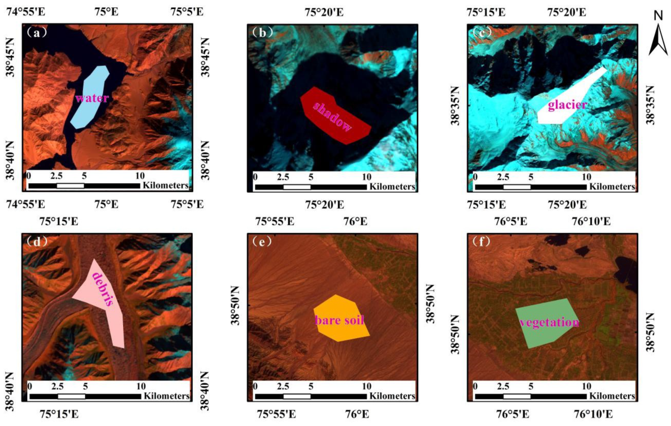
Different land cover classes where training samples were selected based on visual interpretation of the Landsat-8 image. A false-colour composite with a band combination, R = shortwave infrared band (band 6), G = near-infrared band (band 5) and B = blue band (band 2). The letters in rose red indicate water (with pattern in blue) (a), (b) shadow (with pattern in brown), (c) glacier (with pattern in white), (d) debris (with pattern in pink), (e) bare soil (with pattern in orange) and (f) vegetation (with pattern in green).
Figure 8.
Different land cover classes where training samples were selected based on visual interpretation of the Landsat-8 image. A false-colour composite with a band combination, R = shortwave infrared band (band 6), G = near-infrared band (band 5) and B = blue band (band 2). The letters in rose red indicate water (with pattern in blue) (a), (b) shadow (with pattern in brown), (c) glacier (with pattern in white), (d) debris (with pattern in pink), (e) bare soil (with pattern in orange) and (f) vegetation (with pattern in green).

Figure 9.
Preliminary classification results based on the Landsat-8 image acquired on 20 October 2017, using Scheme 3 methods with Random Forest.
Figure 9.
Preliminary classification results based on the Landsat-8 image acquired on 20 October 2017, using Scheme 3 methods with Random Forest.

Figure 10.
Accuracy assessment of land cover classification results.

Figure 11.
Glacial area and elevation with a hillshade view of ASTER GDEM V2 in the background.

Figure 12.
(a) Distribution of glacier number and area, and mean altitude for different size classes; (b) glacier number and area for different mean slopes; (c) glacier number and area for various aspects of the study area; and (d) boxplots of minimum, mean and maximum elevations of the glaciers.
Figure 12.
(a) Distribution of glacier number and area, and mean altitude for different size classes; (b) glacier number and area for different mean slopes; (c) glacier number and area for various aspects of the study area; and (d) boxplots of minimum, mean and maximum elevations of the glaciers.

Figure 13.
Three-dimensional distribution of elevation, slopes, and aspect of the glaciers.

Figure 14.
(a) Distribution of glacier elevation (background: a false-colour composite with a band combination: R = shortwave infrared band (band 6), G = near-infrared band (band 5) and B = blue band (band 2) of the Landsat-8 OLI image acquired on 20 October 2017); and (b) hypsometry of all glaciers in the study area.

Figure 15.
(a–d) Results of the Random Forest classification (yellow lines) compared with those of the three inventories CGI (orange lines), TPG2017 (rose red lines) and CCI (blue lines) with a false color band combination image acquired 20 October 2017, R = shortwave infrared band (band 6), G = near-infrared band (band 5) and B = blue band (band 2).


Table 1.
A list of OLI and TIRS spectral bands of Landsat-8.
| Band | Landsat-8 Operational Land Imagers (OLI) & Thermal Infrared Sensor (TIRS) | ||
|---|---|---|---|
| Name | Wavelength (micrometres) | Resolution (meter) | |
| 1 | Coastal/Aerosol | 0.435–0.451 | 30 |
| 2 | Blue | 0.452–0.512 | 30 |
| 3 | Green | 0.533–0.590 | 30 |
| 4 | Red | 0.636–0.673 | 30 |
| 5 | NIR | 0.851–0.879 | 30 |
| 6 | SWIR1 | 1.566–1.651 | 30 |
| 7 | SWIR2 | 2.107–2.294 | 30 |
| 8 | PAN | 0.503–0.676 | 15 |
| 9 | Cirrus | 1.363–1.384 | 30 |
| 10 | TIR1 | 10.60–11.19 | 100 |
| 11 | TIR2 | 11.50–12.51 | 100 |
NIR, near-infrared; SWIR, shortwave infrared; PAN, panchromatic; TIR, thermal infrared.
Table 2.
List of datasets used in this study.
| Data | Date | Resolution (m) | Utilization |
|---|---|---|---|
| Landsat-8 OLI&TIRS | 20 October 2017 | 30 | Glacier delineation |
| 27 April 2017 | |||
| 13 May 2017 | |||
| ASTER GDEM V2 | 2009 | 30 | Estimation of glacier elevation |
| ITS_LIVE | 1985–2018 | 120,240 | Glacier delineation |
| The second glacier inventory dataset of China (CGI2) | 2006–2011 | Estimation of glacier area change | |
| Tibetan Plateau glacier data—TPG2017 | 2017 | Estimation of glacier area change | |
| Glacier inventory of the Pamir and Karakoram (CCI) | 2018 | Estimation of glacier area change |
Table 3.
Random Forest algorithm parameter setting.
| Name | Explanation | Value |
|---|---|---|
| n_estimators | Maximum number of weak learners (decision trees). | 100 |
| criterion | Criteria for evaluating features when dividing decision trees. The options are “Gini” of Gini Impurity and “entropy” of information gain. | Gini |
| max_features | Maximum number of features considered when dividing. | None |
| max_depth | Decision tree maximum depth. | None |
| min_samples_split | Minimum number of samples required for internal node subdivision. | 10 |
| min_samples_leaf | Minimum number of samples for leaf nodes. | 1 |
Table 4.
Experimental Scheme Information.
| Experimental Scheme | Feature Combination |
|---|---|
| Scheme 1 | Spectral features + Textural features + Temperature features |
| Scheme 2 | Spectral features + Textural features + Temperature features + Topographic features |
| Scheme 3 | Spectral features + Textural features + Temperature features + Topographic features + Movement velocity features |
Table 5.
Accuracy Statistics of Classification Results.
| Classification | Scheme 1 | Scheme 2 | Scheme 3 | |
|---|---|---|---|---|
| Overall Accuracy (%) | 97.42 | 97.43 | 97.60 | |
| Kappa Coefficient | 0.9596 | 0.9598 | 0.9624 | |
| Bare Soil | PA (%) | 96.77 | 96.70 | 96.80 |
| UA (%) | 99.16 | 99.09 | 99.39 | |
| Vegetation | PA (%) | 98.95 | 98.87 | 99.22 |
| UA (%) | 95.93 | 96.00 | 95.84 | |
| Debris | PA (%) | 96.20 | 96.46 | 97.17 |
| UA (%) | 90.19 | 89.82 | 91.59 | |
| Glacier | PA (%) | 96.22 | 96.73 | 96.84 |
| UA (%) | 95.11 | 95.16 | 95.43 | |
| Shadow | PA (%) | 93.13 | 93.81 | 93.36 |
| UA (%) | 96.40 | 97.24 | 97.19 | |
| Water | PA (%) | 99.71 | 99.89 | 99.87 |
| UA (%) | 99.72 | 99.57 | 99.56 | |
PA, producer’s accuracy; UA, user’s accuracy.
Table 6.
The area for each land cover class obtained by the Random Forest classifier.
| Land Cover Class | Area (km2) | Percent (%) |
|---|---|---|
| Bare Soil | 1626.82 | 66.34 |
| Vegetation | 28.27 | 1.15 |
| Debris | 135.46 | 5.52 |
| Glacier | 372.23 | 15.18 |
| Shadow | 283.19 | 11.55 |
| Water | 6.23 | 0.25 |
| Total | 2452.30 | 100 |
Publisher’s Note: MDPI stays neutral with regard to jurisdictional claims in published maps and institutional affiliations. |
© 2020 by the authors. Licensee MDPI, Basel, Switzerland. This article is an open access article distributed under the terms and conditions of the Creative Commons Attribution (CC BY) license (http://creativecommons.org/licenses/by/4.0/).
Share and Cite
MDPI and ACS Style
Lu, Y.; Zhang, Z.; Huang, D. Glacier Mapping Based on Random Forest Algorithm: A Case Study over the Eastern Pamir. Water 2020, 12, 3231. https://doi.org/10.3390/w12113231
AMA Style
Lu Y, Zhang Z, Huang D. Glacier Mapping Based on Random Forest Algorithm: A Case Study over the Eastern Pamir. Water. 2020; 12(11):3231. https://doi.org/10.3390/w12113231
Chicago/Turabian StyleLu, Yijie, Zhen Zhang, and Danni Huang. 2020. "Glacier Mapping Based on Random Forest Algorithm: A Case Study over the Eastern Pamir" Water 12, no. 11: 3231. https://doi.org/10.3390/w12113231
Note that from the first issue of 2016, this journal uses article numbers instead of page numbers. See further details here.