Return Level Analysis of the Hanumante River Using Structured Expert Judgment: A Reconstruction of Historical Water Levels

Abstract

Like other cities in the Kathmandu Valley, Bhaktapur faces rapid urbanisation and population growth. Rivers are negatively impacted by uncontrolled settlements in flood-prone areas, lowering permeability, decreasing channels widths, and waste blockage. All these issues, along with more extreme rain events during the monsoon due to climate change, have led to increased flooding in Bhaktapur, especially by the Hanumante River. For a better understanding of flood risk, the first step is a return level analysis. For this, historical data are essential. Unfortunately, historical records of water levels are non-existent for the Hanumante River. We measured water levels and discharge on a regular basis starting from the 2019 monsoon (i.e., June). To reconstruct the missing historical data needed for a return level analysis, this research introduces the Classical Model for Structured Expert Judgment (SEJ). By employing SEJ, we were able to reconstruct historical water level data. Expert assessments were validated using the limited data available. Based on the reconstructed data, it was possible to estimate the return periods of extreme water levels of the Hanumante River by fitting a Generalized Extreme Value (GEV) distribution. Using this distribution, we estimated that a water level of about 3.5 m has a return period of ten years. This research showed that, despite considerable uncertainty in the results, the SEJ method has potential for return level analyses.

1. Introduction

Flooding has become a major problem in Bhaktapur recently, with the two largest floods on record occurring in 2015 and 2018 [1]. In July 2018, precipitation stations in Bhaktapur recorded the highest amount of rainfall documented in the last decade [1]. This extreme rainfall event caused the Hanumante River to flood the entire area, affecting the local population, blocking transportation and leaving the city in disarray. Bhaktapur is the third biggest city in the Kathmandu Valley (Valley) and is located in the eastern part of the Valley [2]. Like other cities in the Valley, Bhaktapur faces rapid urbanisation and an annual population growth of 2.3 percent in recent years [3]. With this, land use patterns are changing rapidly. According to a study on land use changes by the International Centre for Integrated Mountain Development (ICIMOD), the built area has increased by more than 250% over 20 years [4]. New, unsafe, settlements are emerging within the floodplains and the government lags behind implementing proper land-use policy to control unrestrained settlement [1]. Not only is the river constrained by these uncontrolled settlements, but also insufficient width and freeboard of bridges, and waste blockages cause problems [5]. Due to all these changes, along with more extreme rain events during the monsoon due to climate change, flooding has become a reoccurring problem in Bhaktapur [6].

Flood risk analyses require a sound understanding of how the river behaves. Unfortunately, the Hanumante River is a relatively ungauged river system and little data are available. Only one earlier research concerning the flood risk of the Hanumante River was found: In 2009, the Nepali Department of Water Induced Disaster Prevention created a risk map for the Valley. They used a rainfall-runoff relation for a discharge measurement point at the Bagmati River at Chobar to correlate the rainfall, drainage area and the measured discharge. Then, they used this relation to roughly determine and predict return periods of maximum discharges for locations at different rivers in the Valley, including one location at the Hanumante River [7]. However, a validation of this study based on past flood events was not possible, since historical records of water levels are non-existent. The aim of our research is to fill this gap. Other than our measurements in this study, there are no hydrological stations that have measured water level and discharge within the watershed of the Hanumante River. We measured water levels and discharge on a regular basis only starting from the monsoon months of 2019 together with the non-governmental organization Smartphones For Water Nepal (S4W-Nepal) (https://www.smartphones4water.org/). S4W-Nepal mobilizes mobile technology, citizens and young researchers to collect water data (e.g., rainfall, groundwater levels, water quality) as an alternative for the traditional approach that requires permanent sensors [8]. However, to gain a better understanding of the river system and the corresponding flood risk, data from one monsoon are not sufficient and more historical data are essential.

Due to the lack of data, the Classical Model (CM) for Structured Expert Judgment (SEJ) has been employed [9]. SEJ uses experts’ judgments to quantify the uncertainty for variables of interest. CM objectively evaluates experts’ uncertainty assessments and mathematically aggregates expert probability distributions using performance-based weights. This model is one of the most applied methods of SEJ, with numerous documented studies [10,11,12]. For example, CM has been previously employed as support in the evaluation of levee safety [13] or for the uncertainty analysis of dike ring failure frequency [14]. Other expert judgment methods are available and have been applied in water related topics. For example, the Sheffield method, which aggregates expert input via discussions has been employed to assess the uncertainties of factors affecting high impact and low probability risks for water supply delivery [15].

The aim of CM is to validate experts’ assessments based on how statistically accurate, or calibrated, and informative they are rather than to pre-judge experts prior to processing their assessments. This entails the principle of fairness, which, along with accountability, neutrality and empirical control encompass the four principles of SEJ [9]. Accountability requires all data, including experts’ affiliations and assessments, as well as all processing tools to be open to peer review and results to be reproducible. The names of experts should however not be linked to their assessments in any public output. The principle of neutrality states that the method for evaluating and combining expert opinion should encourage experts to state their true opinions. Finally, empirical control assumes that experts’ assessments are subjected to empirical quality controls. This principle fundamentally differentiates CM from other expert judgment methods, by advocating the same quality control for expert opinion as for empirical data.

What qualifies an individual to be considered an expert is an important, yet unanswered, question in the field of expert judgment. It is generally agreed, however, that input from more experts is desirable. Furthermore, domain knowledge is evidently required, though specific details of what exactly is implied by domain knowledge are, to the best of our knowledge, not provided. The ability to quantify uncertainty requires a complementary set of skills which have shown to not correlate with status or peer valuation [16]. Another recommended best practice is to use a diverse set of experts, where diversity can encompass domain knowledge, demographics, etc. [17].

The validation of experts’ assessments and the fairness principle of the CM lessen some of the burden of expert selection. The same principle of prior performance has been later employed in the good judgment project [18], and which has lead to the so-called superforecasters [19]. Superforecasters emerged from large scale testing for prediction of uncertain events, in which forecasters did not necessarily have what is perceived as considerable domain knowledge. Similarly, in this study, not only specialists in the field of water are considered experts, but also local citizens and students. Their assessments of uncertainty will be evaluated objectively and will be aggregated to obtain distributions for the quantities of interest.

All the aforementioned principles make SEJ arguably the best method to employ for aggregating expert opinion, as the empirical control ensures that expert data are evaluated as any other data. Furthermore, expert judgment methods in general have become a standard approach in risk and decision analysis, when empirical data are incomplete or simply unavailable. In flood risk evaluation, other approaches have been employed in addressing the lack of data, such as historical photographic documentation, aerial photography or satellite images [20,21]. Nonetheless, only a few photographs reporting flood events could be retrieved for the Hanumante river, which was insufficient for our study. Furthermore, to the best of authors’ knowledge, there are no aerial photos available for the Hanumante river. Moreover, the accuracy of aerial photographs or satellite images can be questionable and appear to highly depend on the hydraulic characteristics of the region of interest. The experts of this study, and in particular the citizens living in the area have shown to be very knowledgeable of these characteristics, and their expertise has therefore proven to be highly valuable.

It is common practice to evaluate the flood risk in terms of river discharge and the corresponding return periods. However, for the applicability of SEJ, the assessment of water levels is more suitable, since these are more straightforward to be estimated by the experts. After all, water levels are visually measurable for everyone, whereas discharges are not. So, the overall objective of this research is to evaluate CM as an approach for developing return water levels. This has been investigated by means of a return level analysis for the city of Bhaktapur, in terms of extreme monthly water levels and their corresponding return periods in years. The lack of data has been addressed by employing CM for extreme monthly water levels, which have subsequently been fitted by a Generalized Extreme Value (GEV) distribution to extrapolate the extreme water levels to larger return periods. The fitted GEV distribution describes the behaviour of the extreme water levels as corresponding probabilities and consequently, related risks can be estimated in the future. Despite the large uncertainties, the method shows potential for performing return level analyses in locations where data are sparse or unavailable.

2. Materials and Methods

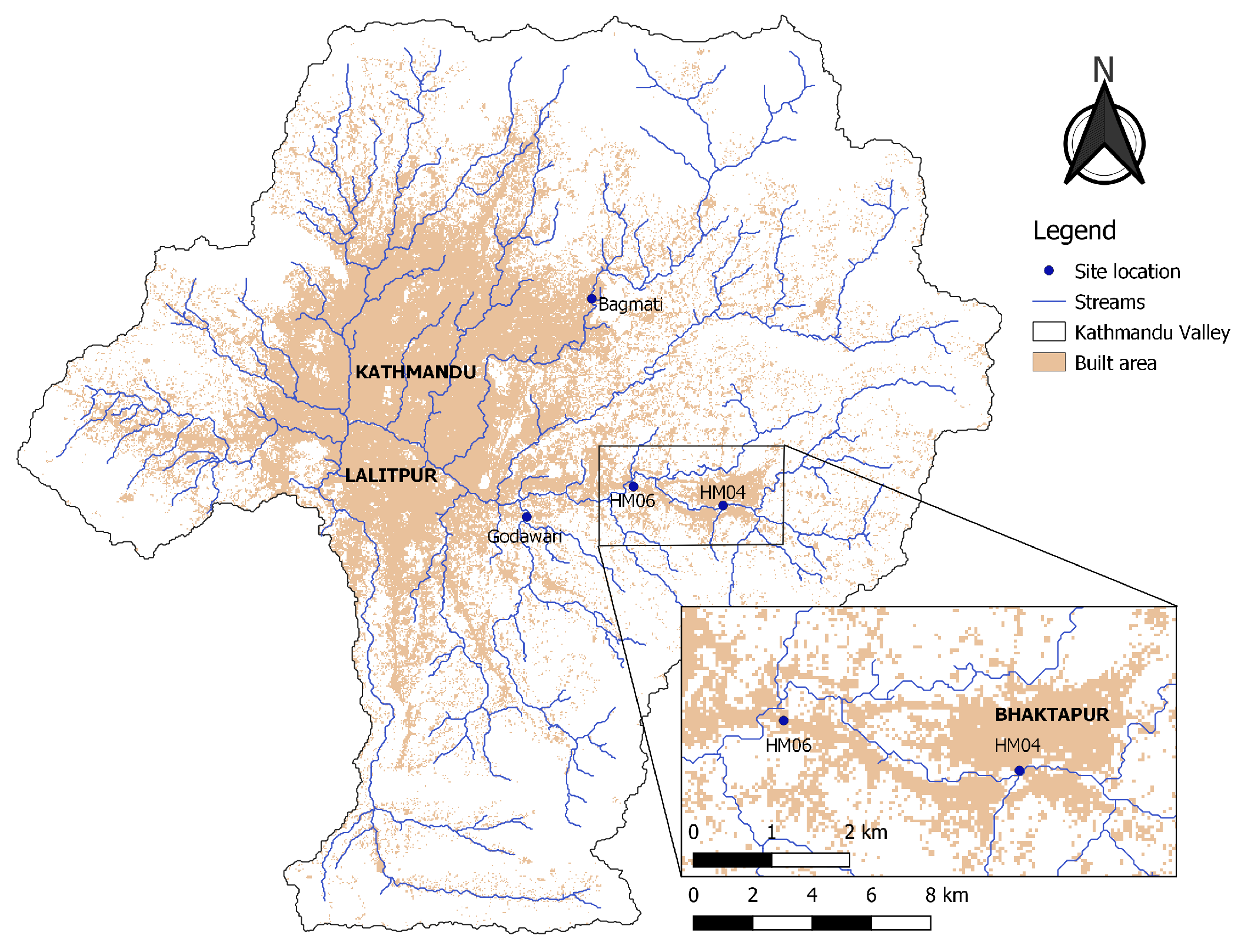
The analysis has been carried out in two parts. First, we used SEJ to estimate water levels of monthly maxima. Second, a GEV distribution was fitted to the resulting time series in order to provide an estimation of the return levels of the Hanumante River.

2.1. Study Area

This research has been conducted in the Bhaktapur Municipality area from August 2019 to October 2019. The municipality of Bhaktapur is located twelve kilometers east of the city of Kathmandu (Figure 1). The town is bounded by the Hanumante River to the south and Khasankhusang river to the northeast. The city spreads over an area of 6.88 square kilometers at an elevation of 1401 m above mean sea level [22].

The Hanumante River (River) is one of the tributaries of the Bagmati River, the main river in the Valley, and has a catchment area of 143 km${}^2$. The major water sources for the Hanumante River are rainfall and natural springs. It is the main natural river in the district of Bhaktapur and the most important water source for the city. Additionally, it is of great ecological, cultural and religious importance. The Hanumante River has multiple tributaries with their own sub-basins [22]. In pre-monsoon months, the River can be almost dry in some areas, while it can transform into a broad and fast-flowing river during monsoon months, with water levels up to two to five meters. The average river width decreased from six in 1964 to two meters in recent times [1]. In the past, the low lands close to the River were only used for agriculture. Now, many people have built their houses in these low areas and some are even located within the River’s flood plains [1]. This resulted in a significant increase of the risk of flooding.

Starting in June 2019, S4W-Nepal measured water levels daily in the Hanumante River at two sites: HM04 and HM06 (see Figure 1). Therefore, the only daily water level data for the Hanumante River that exists is from June, July, and August of 2019. Monthly discharge measurements were also performed during these months. We chose to estimate return levels for HM04, for the following reasons. First, HM04 is located at a bridge that has already been there for several decades, according to local inhabitants. The presence of the bridge ensures that the river width is constant in time at this location, even though the average river width has decreased within Bhaktapur. Secondly, HM04 is located close to the old city center of Bhaktapur. As a result, many citizens know the location and the surrounding area that is prone to flooding.

2.2. Structured Expert Judgment

We used the Classical Model (CM) for structured expert judgment (SEJ) to estimate monthly maximum water levels during the monsoon months for the period 1990–2018. The CM is a rigorous method that evaluates expert opinion based on two objective measures, namely statistical accuracy or calibration score and informativeness, and uses these measures to derive performance-based weights and, in turn, to aggregate assessments [9]. The two measures ensure CM satisfies the empirical control principle listed in the introduction. Within CM, experts are asked to assess their uncertainty for the quantities of interest, denoted as target variables or questions. Moreover, the experts provide uncertain assessments for quantities that are not known to them, but are known to the analysts; these are referred to as seed/calibration questions or variables. The answers to these calibration questions are referred to as realizations.

The target questions referred to unknown monthly maximum water levels for June, July and August, for the time period of interest, at the location HM04. The calibration questions were questions about the water levels that have been measured by S4W-Nepal. Ten calibration questions and 88 questions of interest have been asked in total. The experts were informed which questions were calibration questions and which questions were target questions.

Instead of providing the entire probability distribution for an unknown quantity, experts are asked to specify their uncertainty by providing three quantiles of the distribution, that is the 5%, 50%, and 95% quantile. The 5% quantile is intuitively referred to as a “lower bound”, since, with this statement, the expert believes there is a $5\%$ chance that the true value is below the stated 5% quantile. The 50% quantile or the median is usually referred to as the “best estimate”, for which the expert believes there is a $50\%$ chance the true value is below or above the stated quantile. Finally, the 95% quantile is referred to as an “upper bound”, since the expert believes there is a $95\%$ chance that the true value lies below the stated quantile.

2.2.1. Evaluating Experts’ Assessments

Experts’ assessments have been evaluated by two measures of performance: calibration score (or statistical accuracy) and information score. Formally, for computing the calibration score, an expert is treated as a statistical hypothesis and the calibration score is the p-value that the realizations correspond statistically to expert’s assessments [9]. Suppose an expert is asked one hundred seed questions. Statistically, it is then expected that five times, the realization will fall below the 5% quantile assessments and five times the realization will fall above the 95% quantile assessments. For the other ninety questions the realizations should fall in the second inter-quantile range (ranging from 5% to 50% quantile) and the third inter-quantile range (ranging from 50% to 95% quantile) evenly. The more the expert deviates from these expected frequencies, the lower the calibration score will be. As emphasized by Cooke and Goossens [10], CM does not use hypothesis testing to reject expert hypotheses, but to “measure the degree to which data supports the hypothesis” that expert’s assessments are statistically accurate. The calibration score is determined considering all calibration questions. If the assessments of an expert are perfectly statistically accurate, then the calibration score is 1. The less statistically accurate the assessments of the expert are, the lower the calibration score. The calibration score hence ranges from 0 to 1.

The information score is a measure of the concentration of experts’ assessments with respect to a background measure, which can be a uniform or a logarithmic uniform distribution. We used the uniform distribution as the background measure for this study. The information score measures the discrepancy between the expert’s distribution and the uniform background measure, for which every assessment is considered equally likely [23]. The exact formula is included in the supplementary material. The information score is determined for each question, and can be computed for both calibration questions as well as questions of interest. An overall information score is computed by averaging the information scores over all calibration questions or over all questions in the study. The information score always positive, and the higher the information score, the more informative expert’s assessments are.

Experts’ calibration scores can differ significantly, as it will become apparent for the present study. The information scores do not vary so much, and, compared to the calibration score, can be regarded as a slowly varying function. A detailed description of the two scores is included in the Supplementary Material.

2.2.2. Aggregating Experts’ Assessments

The overall performance of each expert’s assessments is characterised by a combined score, which is the product of the calibration score and the information score for the calibration questions. The combined score is driven by the calibration score, since the information score is a slowly varying function. The normalized combined score provided performance-based weight for each expert. Finally, a weighted combination of experts’ distributions leads to a so-called performance-based Decision Maker (DM): the combination of all the experts’assessments to one combined uncertainty assessment for each question. Since the assessments of all calibration questions are used in determining the weights, the DM is also referred to as the “global weight DM”. Alternatively, weights can be determined for each question, by considering the overall calibration score, but the information score of that particular question. Then, the DM is referred to as the “Item weight DM”.

Experts’ distributions are aggregated for the target questions, but can also be aggregated for the calibration questions. The resulting DM’s assessments can then be assessed with respect to the calibration and information score, just as any expert’s assessments. The two scores can be used to evaluate the performance of the DM. This constitutes the trademark of CM, where not only experts’ assessments, but also aggregated assessments are subjected to the two objective measures of evaluation.

The resulting combined score of the DM can be used in an expert selection optimized procedure. This approach answers the question of which expert selection leads to best possible aggregated performance, i.e., the highest combined score. The calibration score is used as a criterion for the selection of the pool of experts and the significance level $\alpha \ge 0$ formalizes the selection procedure. The resulting DM of this procedure is referred to as the “Optimized DM”. Other weights are possible, for example, one can consider equal weights, which lead to the so-called “equal weight DM”. A more elaborate description of the different DM’s can be found in the Supplementary material.

2.2.3. Expert Selection & Questionnaires

As mentioned, the Hanumante River has not to been studied extensively by hydrologists. This general lack of knowledge for the Hanumante River made the selection of domain experts challenging. We addressed this challenge by engaging a large and diverse pool of experts for this study: hydrologists, engineers working for water related governmental institutions, young S4W-Nepal researchers, but also citizens who live or work closely to the river. The aim was to have at least ten assessments by specialists in the field of water. Recall that CM relies on the objective evaluation of expert assessments, which entangles domain expertise with uncertainty quantification. Domain expertise is therefore necessary yet not sufficient in assessing water levels. All our participants in the study will be further referred to as “experts”, and those who have specialized domain knowledge will be referred to as “specialists”.

We conducted elicitations with 62 experts in September 2019 in the city of Bhaktapur through interviews and an online survey. Some details of the experts can be found in

Table 1. Overview of the experts who participated in the elicitation in September 2019.

		Panels
Function	Total	1	2	3	4
Number of experts	62	16	16	16	14
Number of specialists	10	1	2	4	3
Number of citizens	47	13	13	11	10
Number of students	5	2	1	1	1
Average age	35.8	39.6	32.8	34.4	36.3
Male/Female	41/21	8/8	11/5	11/5	11/3

. The majority of the experts in the study were citizens of Bhaktapur, meaning that they live and/or work close to the Hanumante River. Most of these people were shop owners and school teachers. The specialists were employees at the Nepali governmental Department of Hydrology and Meteorology (DHM), staff at the Kwopa College of Engineering in Bhaktapur and other water researchers that live or have lived in the Kathmandu Valley. Also, some students in the field of water and/or Civil Engineering participated.

As mentioned before, the aim of the SEJ was to create a time series of extreme monthly water levels of the Hanumante River that could be used for a return level analysis. In order to reliably determine statistics (i.e., return levels) from a time series, it is important to have a time series that is sufficiently long. We decided that the time series should cover the monsoon months of June, July and August for the period 1990–2019. This led to at least ninety target questions that the experts would have need to provide assessments for. To prevent such a large number of elicited questions for the experts, we split the target questions over four panels and distributed the 62 experts over the panels. We ensured that the diversity of expertise was distributed more or less uniformly across panels, with at least two specialists to each panel.

Table A1. Overview questions per panel.

		Specific Question Number Per Group
Question nr	Question	Validation Panel	Panel 1	Panel 2	Panel 3	Panel 4
CQ1	What was the highest water level at the Bagmati River in July 2017?	1	1	1	1	1
CQ2	What was the highest water level at the Godawari River in July 2017?	2	2	2	2	2
CQ3	What was the highest water level at the HM06 in July 2018?	3	3	3	3	3
CQ4	What was the highest water level at the HM06 in June 2019?	4	4	4	4	4
CQ5	What was the highest water level at the HM06 in July 2019?	5	5	5	5	5
CQ6	What was the highest water level at the HM06 in August 2018?	6	6	6	6	6
CQ7	What was the highest water level at the HM04 in August 2015?	7	7	7	7	7
CQ8	What was the highest water level at the HM04 in August 2019?	8	8	8	8	8
CQ9	What was the highest water level at the HM04 in July 2019?	9	9	9	9	9
CQ10	What was the highest water level at the HM04 in June 2019?	10	10	10	10	10
TQ1	What was the highest water level in August 2018?	11	11	11	11	11
TQ2	What was the highest water level in July 2018?	12	12	12	12	12
TQ3	What was the highest water level in June 2018?	13	13	13	13	13
TQ4	What was the highest water level in August 2017?		14
TQ5	What was the highest water level in July 2017?		15
TQ6	What was the highest water level in June 2017?		16
TQ7	What was the highest water level in August 2016?			14
TQ8	What was the highest water level in July 2016?			15
TQ9	What was the highest water level in June 2016?			16
TQ10	What was the highest water level in August 2015?				14
TQ11	What was the highest water level in July 2015?				15
TQ12	What was the highest water level in June 2015?				16
TQ13	What was the highest water level in August 2014?					14
TQ14	What was the highest water level in July 2014?					15
TQ15	What was the highest water level in June 2014?					16
TQ16	What was the highest water level in August 2013?		17
TQ17	What was the highest water level in July 2013?		18
TQ18	What was the highest water level in June 2013?		19
TQ19	What was the highest water level in August 2012?			17
TQ20	What was the highest water level in July 2012?			18
TQ21	What was the highest water level in June 2012?			19
TQ22	What was the highest water level in August 2011?				17
TQ23	What was the highest water level in July 2011?				18
TQ24	What was the highest water level in June 2011?				19
TQ25	What was the highest water level in August 2010?					17
TQ26	What was the highest water level in July 2010?					18
TQ27	What was the highest water level in June 2010?					19
TQ28	What was the highest water level in August 2009?		20
TQ29	What was the highest water level in July 2009?		21
TQ30	What was the highest water level in June 2009?		22
TQ31	What was the highest water level in August 2008?			20
TQ32	What was the highest water level in July 2008?			21
TQ33	What was the highest water level in June 2008?			22
TQ34	What was the highest water level in August 2007?				20
TQ35	What was the highest water level in July 2007?				21
TQ36	What was the highest water level in June 2007?				22
TQ37	What was the highest water level in August 2006?					20
TQ38	What was the highest water level in July 2006?					21
TQ39	What was the highest water level in June 2006?					22
TQ40	What was the highest water level in August 2005?	14	23	23	23	23
TQ41	What was the highest water level in July 2005?	15	24	24	24	24
TQ42	What was the highest water level in June 2005?	16	25	25	25	25
TQ43	What was the highest water level in August 2004?		26
TQ44	What was the highest water level in July 2004?		27
TQ45	What was the highest water level in June 2004?		28
TQ46	What was the highest water level in August 2003?			26
TQ47	What was the highest water level in July 2003?			27
TQ48	What was the highest water level in June 2003?			28
TQ49	What was the highest water level in August 2002?				26
TQ50	What was the highest water level in July 2002?				27
TQ51	What was the highest water level in June 2002?				28
TQ52	What was the highest water level in August 2001?					26
TQ53	What was the highest water level in July 2001?					27
TQ54	What was the highest water level in June 2001?					28
TQ55	What was the highest water level in August 2000?		29
TQ56	What was the highest water level in July 2000?		30
TQ57	What was the highest water level in June 2000?		31
TQ58	What was the highest water level in August 1999?			29
TQ59	What was the highest water level in July 1999?			30
TQ60	What was the highest water level in June 1999?			31
TQ61	What was the highest water level in August 1998?				29
TQ62	What was the highest water level in July 1998?				30
TQ63	What was the highest water level in June 1998?				31
TQ64	What was the highest water level in August 1997?					29
TQ65	What was the highest water level in July 1997?					30
TQ66	What was the highest water level in June 1997?					31
TQ67	What was the highest water level in August 1996?		32
TQ68	What was the highest water level in July 1996?		33
TQ69	What was the highest water level in June 1996?		34
TQ70	What was the highest water level in August 1995?			32
TQ71	What was the highest water level in July 1995?			33
TQ72	What was the highest water level in June 1995?			34
TQ73	What was the highest water level in August 1994?				32
TQ74	What was the highest water level in July 1994?				33
TQ75	What was the highest water level in June 1994?				34
TQ76	What was the highest water level in August 1993?					32
TQ77	What was the highest water level in July 1993?					33
TQ78	What was the highest water level in June 1993?					34
TQ79	What was the highest water level in August 1992?		35
TQ80	What was the highest water level in July 1992?		36
TQ81	What was the highest water level in June 1992?		37
TQ82	What was the highest water level in August 1991?			35
TQ83	What was the highest water level in July 1991?			36
TQ84	What was the highest water level in June 1991?			37
TQ85	What was the highest water level in August 1990?	17	38	38	35	35
TQ86	What was the highest water level in July 1990?	18	39	39	36	36
TQ87	What was the highest water level in June 1990?	19	40	40	37	37
TQ88	What do you expect to be the highest water level in the year 2025?	20	41	41	38	38

in Appendix A, includes an overview of the different questions asked in the different panels.

To investigate whether the assessments across panels exhibit systematic differences, we included nine overlapping target questions for all panels. The overlapping questions were answered by all 62 experts and were grouped into another distinct panel, which is referred to as the validation panel. The resulting DM’s performance for the validation panel was then compared to the DM’s performance for the four panels, to investigate whether there are clear distinctions between the panels. Eventually, every questionnaire for each expert consisted of ten calibration questions and 28 or 31 target variables (including the overlapping questions).

The importance of explanation and communication of the method was regarded to be a key factor for the experts’ elicitation. We performed individual expert elicitations. A translator was present during the elicitation and an elaborate explanation of the method was provided before the elicitation. Moreover, an example question was also provided to ensure that the experts understand the method and process. Thirteen of the specialists gave their responses via an online survey. We informed these experts about the method beforehand.

2.2.4. Calibration Questions & Target Questions

For the calibration questions, information about monthly maxima recorded at two locations on the Hanumante River has been used. Furthermore, S4W-Nepal provided data of water levels for a few other locations. Four different sites in the Valley have been chosen for the elicitation. Additionally to the site HM04, HM06 and two other sites, on the Bagmati River and the Godawari river (Figure 1), were considered for as calibration questions. This was done because of a lack of sufficient data points for the Hanumante River. These different sites all featured water level staff gauges that were attached to familiar bridges that could be used as local reference points for the questionnaires. A total of ten calibration questions is typically considered to be sufficient within SEJ studies [10].

We aimed to make the questions as clear and concise as possible and provided the experts with enough background information to estimate the water levels. The background information given in the questionnaires consisted of (1) a map and description of the site location, (2) a picture of the site location, (3) the average water level during the monsoon, and (4) the water level at which the bridge would be inundated. This information was obtained partially from the S4W-Nepal data and partially from site visits and field measurements. Eventually, the calibration questions and the target questions were constructed as: “What was the highest water level in [month][year]?”. An example of the questionnaire is included in the Supplementary Material.

2.2.5. Software

We used ANDURIL to perform the SEJ analysis. ANDURIL is a MATLAB toolbox that implements CM, and includes an extensive list of functions that evaluate the performances of several DM’s [24].

2.3. Return Levels

Employing CM resulted in a time series of maximum monthly water levels for the monsoon for the site HM04, based on estimations of experts. These monthly maxima were converted to yearly maxima. The final objective was to determine the probability of extreme water level events in the future. The most convenient way to express these probabilities is by using return levels. A return level is a water level with a corresponding average occurrence of once every X years, where X is called the return period.

Finding probabilities of extreme events can be achieved by plotting the histogram of the observations and by finding the best fitting parametric probability density function. The commonly used parametric family of distributions is the GEV distribution [25]. That is because the maximum of a sample of independent and identically distributed random variables converges in distribution to a GEV distribution [26]. This asymptotic distribution enables us to extrapolate the data to water levels that are higher than any yet observed value.

There are three widely known and applied GEV distributions within extreme value theory: Gumbel (type I), Fréchet (type II), and reverse Weibull (type III). The most important difference between the various types is that type I is defined for the range ($-\infty$,$+\infty$), type II is bounded for maxima by a lower bound and type III is bounded for maxima by an upper bound [25]. The cumulative distribution function of the GEV distribution is given by

$$F_{GEV}\left(x\right)=\{\begin{array}{cc}\exp \left\{-{[1+\xi \alpha (x-u)]}^{-1/\xi }\right\}& \mathrm{for}\xi \ne 0\\ \exp \left\{-\exp (-\alpha (x-u\left)\right)\right\}& \mathrm{for}\xi =0\end{array}$$

(1)

where

• $\xi =$ 0 Gumbel (Type I for maxima)
• $\xi >$ 0 Fréchet (Type II for maxima)
• $\xi <$ 0 Reverse Weibull (Type III for maxima)

Each GEV type is characterised by a location parameter u, a scale parameter $\alpha$, and a shape parameter $\xi$ [25], which are different for every type. An overview of the properties of the three types, including the typical shape of their distribution functions, is given in the Supplementary material. MATLAB features the built-in function ’gevfit’, which provides maximum likelihood estimates of these shape, scale and location parameters, obtained based on the maximum water level data. The estimated value of the shape parameter $\xi$ yields the type of the best-fitting GEV distribution for the extreme water level data.

The underlying relation between the GEV distribution, water levels, and corresponding return periods is then expressed as follows

$$F_{GEV}\left(Z_p\right)=1-p,$$

(2)

where $F_{GEV}$ is the cumulative distribution function of the best-fitting GEV, $Z_p$ is the return level, and the return period is defined as $1/p$, where p is the probability of occurrence of a return level $Z_p$.

We used the resulting MATLAB estimates of the three parameters to plot the inverse of the GEV, using MATLAB’s built-in function ‘gevinv’. This function returns the inverse cumulative distribution function of the GEV distribution, which provides the expected return water level for a given return period.

Once the probabilities of certain water levels are known, the first step in a flood risk analysis is complete. Risk is often defined as the probability of occurrence p of a given water level multiplied by the consequence of this water level [27]. The lower the acceptable probability p, and thus the higher the return period $1/p$, the safer the area. Consequently, the flood defences surrounding that area can be designed for a chosen acceptable risk, that can be translated into a corresponding (acceptable) return water level. In other words, when an area is hypothetically allowed to be flooded only once every hundred years, the flood defences should be at least as high as the water level that corresponds to this return period of a hundred years. However, this research only focuses on the first step towards a flood risk analysis, namely on estimating the probabilities p of occurrence of certain water levels. Quantifying the consequences could be the subject of a future research.

3. Results

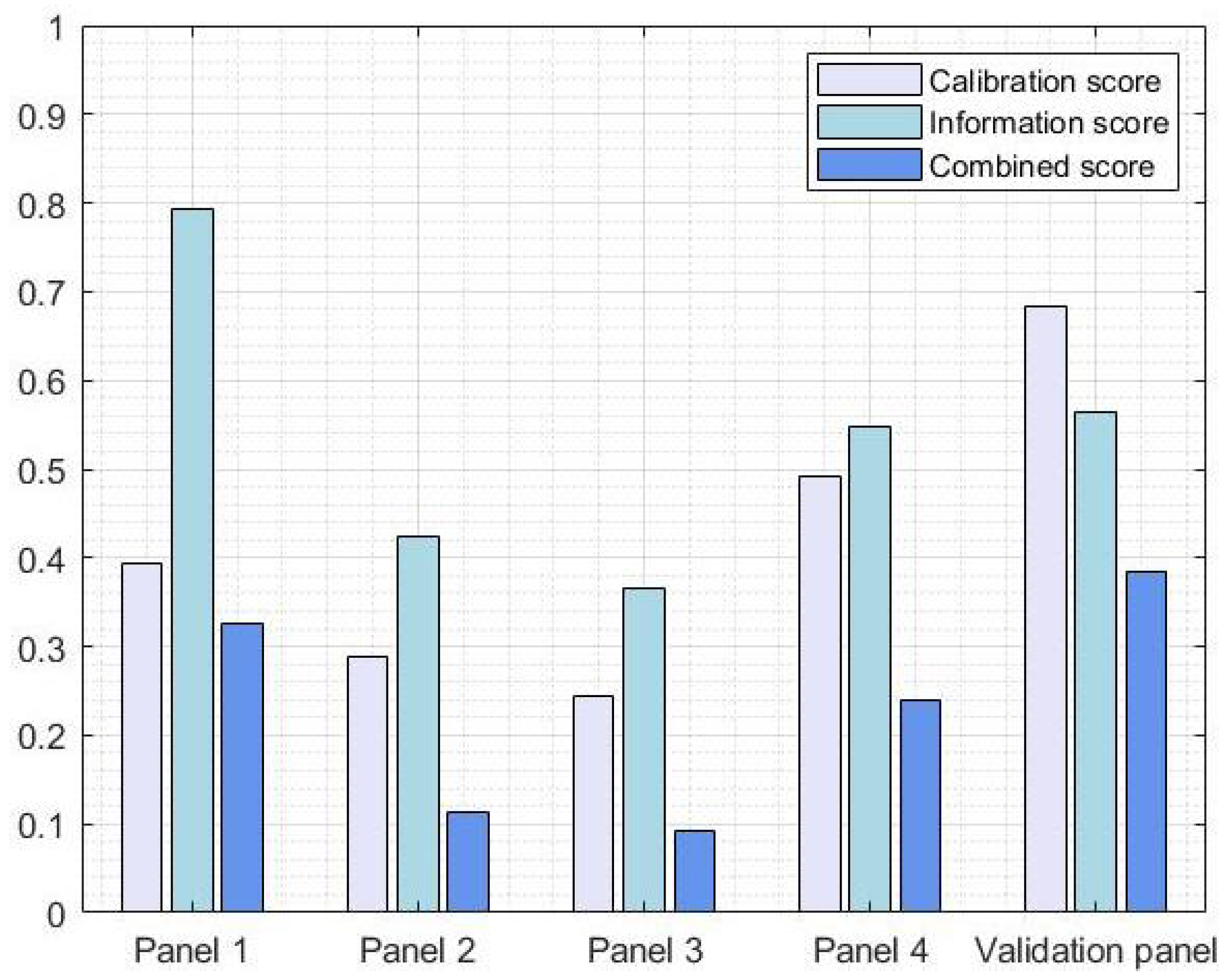
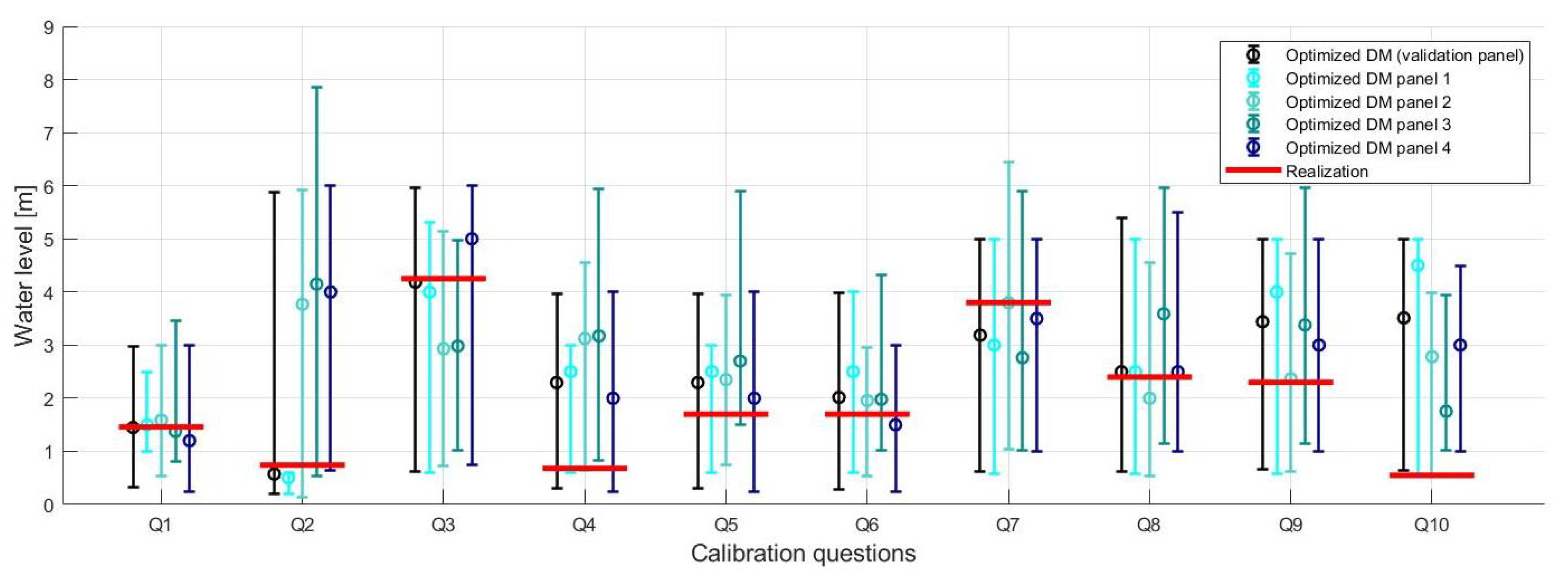
3.1. Structured Expert Judgment

In this section the SEJ results are presented for every panel, including the validation panel. As mentioned in the previous section, experts’ aggregated assessments, or DM’s, can be subjected to the two performance measures, just as any expert. We account for four different aggregation techniques, by using equal weights, performance-based weights computed from all calibration questions, which are referred to as global weights and performance-based weights computed for each question, denoted as item weights. Finally, am optimized DM is constructed for each panel, which reveals the best performing subset of experts within each panel. Experts’ individual scores, as well as their weights within the global and the optimzied DM are presented in Appendix B.

3.1.1. Panel 1

The calibration scores for the experts within panel 1 range from $6.13\times {10}^{-13}$ to $0.395$. The information scores vary from $0.356$ to $2.118$ for the calibration questions and from $0.395$ to $1.981$ for all questions. For nine of the experts, the information scores are (slightly) lower for all questions, suggesting higher uncertainty for the questions of interest as compared to the calibration questions.

Table A2. Calibration and Information scores for experts in panel 1.

Expert	Function	Calibration Score	Information Score (Seed)	Information Score (All)	Normalized Global Weights	Normalized Optimized Weights
Expert 1.1	Citizen of Bhaktapur	$6.085\times {10}^{-2}$	2.118	1.981	0.148	0
Expert 1.2	Student	$1.371\times {10}^{-8}$	2.300	1.893	$3.623\times {10}^{-8}$	0
Expert 1.3	Citizen of Bhaktapur	0.113	0.664	0.680	0.087	0
Expert 1.4	Citizen of Bhaktapur	0.314	0.789	0.460	0.284	0
Expert 1.5	Citizen of Bhaktapur	$1.293\times {10}^{-10}$	1.633	1.503	$2.425\times {10}^{-10}$	0
Expert 1.6	Citizen of Bhaktapur	$1.497\times {10}^{-11}$	1.517	1.172	$2.611\times {10}^{-11}$	0
Expert 1.7	Citizen of Bhaktapur	$6.131\times {10}^{-13}$	1.398	1.010	$9.848\times {10}^{-13}$	0
Expert 1.8	Citizen of Bhaktapur	$6.174\times {10}^{-9}$	1.154	1.255	$8.187\times {10}^{-9}$	0
Expert 1.9	Citizen of Bhaktapur	$2.638\times {10}^{-4}$	0.774	0.843	$2.346\times {10}^{-4}$	0
Expert 1.10	Citizen of Bhaktapur	$1.293\times {10}^{-10}$	1.277	1.298	$1.897\times {10}^{-10}$	0
Expert 1.11	Citizen of Bhaktapur	0.395	0.829	0.795	0.376	1
Expert 1.12	Citizen of Bhaktapur	$1.150\times {10}^{-3}$	0.694	0.625	$9.176\times {10}^{-4}$	0
Expert 1.13	Citizen of Bhaktapur	$3.098\times {10}^{-3}$	0.438	0.510	$1.558\times {10}^{-3}$	0
Expert 1.14	Citizen of Bhaktapur	$6.131\times {10}^{-13}$	2.032	1.847	$1.432\times {10}^{-12}$	0
Expert 1.15	Student	0.228	0.356	0.395	0.093	0
Expert 1.16	Water specialist	$6.289\times {10}^{-3}$	1.301	1.580	$9.403\times {10}^{-3}$	0

in Appendix B includes the calibration and information scores, as well as experts’ weights in the global and optimized DM. An optimized performance-based combination of weights leads to an $\alpha$-value of $0.395$ in which only one expert receives a non-zero weight. This expert is a local shop owner in Bhaktapur.

The results of the different DM’s are summarized in

Table 2. Performance of the different Decision Makers (DM’s) for panel 1.

	Calibration Score	Information Score	Combined Score
Optimized DM	0.3946	0.8287	0.3270
Global weight DM	0.2894	0.2717	0.0786
Item weight DM	0.4735	0.4038	0.1912
Equal weight DM	0.0012	0.1405	0.0002

. We note first that all DM’s except the equal weight DM obtain a calibration score higher than the significance level of 0.05. This suggest that, within a hypothesis testing framework, for EWDM there is enough evidence that its assessments are not statistically accurate. Furthermore, the highest informative DM is the optimized DM, which is also the DM with the highest combined score. Concluding, the optimized DM is the best performing DM for panel 1 and we therefore used the assessments of the optimized DM for the target questions.

3.1.2. Panel 2

Within panel 2, the calibration scores range from $6.17\times {10}^{-9}$ to $0.06085$. From

Table A3. Calibration and Information scores for the experts of panel 2.

Expert	Function	Calibration Score	Information Score (Seed)	Information Score (All)	Normalized Global Weights	Normalized Optimized Weights
Expert 2.1	Citizen of Bhaktapur	$7.994\times {10}^{-4}$	1.466	1.234	$1.177\times {10}^{-2}$	$1.185\times {10}^{-2}$
Expert 2.2	Citizen of Bhaktapur	$6.085\times {10}^{-2}$	0.915	1.093	0.560	0.563
Expert 2.3	Citizen of Bhaktapur	$4.488\times {10}^{-7}$	0.925	1.287	$4.167\times {10}^{-6}$	0
Expert 2.4	Citizen of Bhaktapur	$7.284\times {10}^{-4}$	0.799	0.939	$5.848\times {10}^{-3}$	0
Expert 2.5	Citizen of Bhaktapur	$6.174\times {10}^{-9}$	0.708	0.602	$4.390\times {10}^{-8}$	0
Expert 2.6	Citizen of Bhaktapur	$6.174\times {10}^{-9}$	1.190	1.225	$7.376\times {10}^{-8}$	0
Expert 2.7	Citizen of Bhaktapur	$4.704\times {10}^{-2}$	0.602	0.529	0.284	0.286
Expert 2.8	Citizen of Bhaktapur	$4.937\times {10}^{-7}$	1.537	1.292	$7.620\times {10}^{-6}$	0
Expert 2.9	Citizen of Bhaktapur	$1.543\times {10}^{-7}$	0.769	0.835	$1.192\times {10}^{-6}$	0
Expert 2.10	Water specialist	$2.389\times {10}^{-8}$	1.294	0.653	$3.105\times {10}^{-7}$	0
Expert 2.11	Citizen of Bhaktapur	$5.992\times {10}^{-3}$	1.894	1.664	0.114	0.115
Expert 2.12	Citizen of Bhaktapur	$2.500\times {10}^{-6}$	1.107	1.650	$2.780\times {10}^{-5}$	0
Expert 2.13	Citizen of Bhaktapur	$1.543\times {10}^{-7}$	0.952	0.951	$1.473\times {10}^{-6}$	0
Expert 2.14	Citizen of Bhaktapur	$1.543\times {10}^{-7}$	0.892	1.001	$1.382\times {10}^{-6}$	0
Expert 2.15	Student	$2.083\times {10}^{-5}$	1.429	1.289	$2.990\times {10}^{-4}$	0
Expert 2.16	Water specialist	$1.311\times {10}^{-3}$	1.855	1.656	$2.441\times {10}^{-2}$	$2.456\times {10}^{-2}$

in Appendix B, it can be observed that the assessments of experts of panel 2 are less statistically accurate than the assessments of experts in panel 1. The information scores for seed variables vary from 0.602 to 1.894, and those for all questions vary from 0.529 to 1.656, which are comparable to the results of panel 1. We also computed the optimized DM for panel 2. With an $\alpha$-value of $0.047$, five experts are granted a non-zero weighting, from which four are citizens of Bhaktapur.

The results of the different computed DM’s are summarized in

Table 3. Performance of the different Decision Makers for panel 2.

	Calibration Score	Information Score	Combined Score
Optimized DM	0.2894	0.3924	0.1136
Global weight DM	0.1242	0.4819	0.0599
Item weight DM	0.2441	0.4974	0.1214
Equal weight DM	0.0031	0.1475	0.0005

. It is remarkable that the calibration scores of all DM’s are quite low, but still above the 0.05 significance level threshold, which is the result of the low calibration scores of the experts. Another remarkable observation is that the DM based on item weights has a slightly higher combined score compared to the optimized DM. However, it was decided to use the optimized DM’s results during this research, since the difference in combined scores is negligibly small.

3.1.3. Panel 3

In the third panel, the calibration scores for the experts range from $6.13\times {10}^{-13}$ to $0.036$ (see

Table A4. Calibration and Information scores for the experts of panel 3.

Expert	Function	Calibration Score	Information Score (Seed)	Information Score (All)	Normalized Global Weights	Normalized Optimized Weights
Expert 3.1	Citizen of Bhaktapur	$9.855\times {10}^{-7}$	1.109	1.059	$2.608\times {10}^{-5}$	0
Expert 3.2	Citizen of Bhaktapur	$6.131\times {10}^{-13}$	1.859	1.575	$2.720\times {10}^{-11}$	0
Expert 3.3	Citizen of Bhaktapur	$1.293\times {10}^{-10}$	1.195	1.253	$3.687\times {10}^{-9}$	0
Expert 3.4	Citizen of Bhaktapur	$1.293\times {10}^{-10}$	1.336	1.118	$4.121\times {10}^{-9}$	0
Expert 3.5	Citizen of Bhaktapur	$3.574\times {10}^{-2}$	0.650	0.588	0.555	0.573
Expert 3.6	Citizen of Bhaktapur	$2.042\times {10}^{-3}$	0.434	0.510	$2.115\times {10}^{-2}$	0
Expert 3.7	Citizen of Bhaktapur	$1.293\times {10}^{-10}$	1.643	1.620	$5.071\times {10}^{-9}$	0
Expert 3.8	Citizen of Bhaktapur	$8.214\times {10}^{-3}$	0.845	0.987	0.166	0.171
Expert 3.9	Citizen of Bhaktapur	$1.579\times {10}^{-5}$	0.995	0.906	$3.750\times {10}^{-4}$	0
Expert 3.10	Citizen of Bhaktapur	$1.543\times {10}^{-7}$	0.904	0.831	$3.3.331\times {10}^{-6}$	0
Expert 3.11	Water specialist	$1.543\times {10}^{-7}$	0.746	0.473	$2.747\times {10}^{-6}$	0
Expert 3.12	Citizen of Bhaktapur	$7.284\times {10}^{-4}$	0.625	0.562	$1.087\times {10}^{-2}$	0
Expert 3.13	Water specialist	$6.131\times {10}^{-13}$	2.423	2.407	$3.546\times {10}^{-11}$	0
Expert 3.14	Student	$3.500\times {10}^{-8}$	2.038	1.647	$1.703\times {10}^{-6}$	0
Expert 3.15	Water specialist	$1.066\times {10}^{-6}$	2.284	2.323	$5.812\times {10}^{-5}$	0
Expert 3.16	Water specialist	$6.289\times {10}^{-3}$	1.645	1.120	0.247	0.255

in Appendix B). Compared to the first and second panel, the highest individual calibration score for panel 3 is relatively low. No notable differences in information scores are noticed with the previous panels, except a few high information scores which are coupled with very low calibration scores. This suggest that the experts are quite certain about the range of plausible values, but not statistically accurate, which is usually referred to as overconfidence. When we computed the optimized DM, an $\alpha$-value of $0.0063$ was found, resulting in three experts with non-zero weights, from which two are citizens of Bhaktapur.

The results of the different DM’s are again summarized in

Table 4. Performance of the different Decision Makers for panel 3.

	Calibration Score	Information Score	Combined Score
Optimized DM	0.2441	0.3739	0.0913
Global weight DM	0.0357	0.6502	0.0232
Item weight DM	0.0357	0.6502	0.0232
Equal weight DM	0.0012	0.1542	0.0002

. It can be observed that the calibration score for the optimized DM is still relatively low, of 0.2441, but much higher than any of the expert’s calibration score. Also, compared to the calibration scores of the other DM’s, this value is significantly better. Consequently, the optimized DM obtained the highest combined score and its assessments have been further used in our analysis.

3.1.4. Panel 4

The calibration scores for the experts within the final panel range from $1.29\times {10}^{-10}$ to $0.493$ (see

Table A5. Calibration and Information scores for the experts of panel 4.

Expert	Function	Calibration Score	Information Score (Seed)	Information Score (All)	Normalized Global Weights	Normalized Optimized Weights
Expert 4.1	Citizen of Bhaktapur	$5.992\times {10}^{-3}$	0.722	1.110	$1.590\times {10}^{-2}$	0
Expert 4.2	Citizen of Bhaktapur	$1.293\times {10}^{-10}$	1.192	1.832	$5.660\times {10}^{-10}$	0
Expert 4.3	Citizen of Bhaktapur	0.493	0.485	0.547	0.877	1
Expert 4.4	Citizen of Bhaktapur	$5.544\times {10}^{-2}$	0.228	0.252	$4.649\times {10}^{-2}$	0
Expert 4.5	Citizen of Bhaktapur	$4.488\times {10}^{-7}$	1.172	1.361	$1.933\times {10}^{-6}$	0
Expert 4.6	Citizen of Bhaktapur	$1.293\times {10}^{-10}$	1.684	1.757	$7.999\times {10}^{-10}$	0
Expert 4.7	Citizen of Bhaktapur	$1.628\times {10}^{-4}$	0.811	0.912	$4.850\times {10}^{-4}$	0
Expert 4.8	Citizen of Bhaktapur	$3.321\times {10}^{-2}$	0.483	0.424	$5.999\times {10}^{-2}$	0
Expert 4.9	Citizen of Bhaktapur	$1.893\times {10}^{-6}$	2.119	2.269	$1.473\times {10}^{-5}$	0
Expert 4.10	Water specialist	$1.293\times {10}^{-10}$	1.908	2.282	$9.064\times {10}^{-10}$	0
Expert 4.11	Student	$1.293\times {10}^{-10}$	1.706	1.607	$8.105\times {10}^{-10}$	0
Expert 4.12	Citizen of Bhaktapur	$1.579\times {10}^{-5}$	1.916	1.286	$1.112\times {10}^{-4}$	0
Expert 4.13	Water specialist	$4.937\times {10}^{-7}$	2.733	2.717	$4.958\times {10}^{-6}$	0
Expert 4.14	Water specialist	$2.638\times {10}^{-4}$	0.567	0.763	$5.493\times {10}^{-4}$	0

in Appendix B). The average information scores are 1.37 based on all variables and 1.27 based on the seed variables. The information scores range from and 0.228 to 2.733 for calibration questions. Moreover, 10 experts exhibit lower uncertainty in the questions of interest, as revealed by the higher information scores for all questions than for the calibration questions. When we computed the optimized DM, an $\alpha$-value of $0.493$ was found. Consequently, only one expert received a non-zero weight. Just as in panel 1, this is a local shop owner from Bhaktapur.

The results of the other computed DM’s are summarized in

Table 5. Performance of the different Decision Makers for panel 4.

	Calibration Score	Information Score	Combined Score
Optimized DM	0.4926	0.4848	0.2388
Global weight DM	0.4926	0.3015	0.1485
Item weight DM	0.4926	0.3109	0.1531
Equal weight DM	0.0237	0.1489	0.0035

. Similar to panel 1 and 3, the optimized DM is performing best when compared to the other DM’s. Again notice the low calibration and information score for the equal weight DM.

3.1.5. Validation Panel

For the validation panel, we considered all 62 experts and determined the four different DM’s. In

Table 6. Performance of the different Decision Makers for all 62 experts.

	Calibration Score	Information Score	Combined Score
Optimized DM	0.6828	0.5644	0.3854
Global weight DM	0.2894	0.3542	0.1025
Item weight DM	0.4735	0.4671	0.2212
Equal weight DM	0.0012	0.2487	0.0003

, their corresponding scores are presented. It can be observed that the optimized DM again performs the best, with a relatively high calibration score of 0.6828. For the optimized DM, the $\alpha$-value was equal to 0.3946. This optimized DM included only two experts. Not surprisingly, these were the same experts that were selected for panel 1 and 4 for the optimized DM’s.

For an overall comparison between the panels’ performance, we compared the calibration scores, information scores and combined scores of the optimized DM’s of the individual panels and the validation panel. The results are presented in Figure 2. It shows that the optimized DM of the validation panel performs best when compared to the optimized DM’s of the individual panels. Therefore, the validation panel’s optimized DM has been used for the overlapping questions. Panel 1 is the most informative and the validation panel is the most statistically accurate and the second best informative.

To investigate for systematic differences in the four different panels and in the validation panel, a comparison of DMs assessments is made for the aggregated assessments of the calibration questions, see Figure 3. The horizontal lines indicate the realization for each calibration question, which are the measured water levels. Furthermore the estimates, given by the optimized DM, per panel, including the 5% and 95% quantiles are included. It is remarkable that all but four DMs 90% confidence intervals capture the true water levels. Nonetheless, some intervals are quite wide, denoting high uncertainty in experts’ assessments. Moreover, the median estimates are close to the realization for all DMs for Q1, and Q5–Q9. The largest error in estimating the true value is registered for the calibration questions Q4 and Q10. Both questions were about June 2019, for the locations HM04 and HM06.

There are no panels significantly over- or underestimating when compared to the validation panel. Based on this analysis, we have decided to combine the water levels estimated by the four panels for different years into one data set containing all water levels of the years 1990 until 2019.

We included 9 target questions that have been answered by all 62 experts. In Figure 4, the results of the overlapping questions for the different optimized DM’s are shown. Moreover, the month and the year that concerned each question are included in the x-axis of the figure. It can be seen that the difference in the distribution and in the median assessments is relatively small for the first 6 questions. For the last three questions, the optimized DM in panel 1 and validation panel exhibit distinct distributions than the DM’s from the other three panels. As mentioned beforehand, the optimized DM for the validation panel only takes into account 2 experts, from panel 1 and 4. The fact that the expert from panel 1 gave relatively low assessments with a narrow confidence interval for the last last three questions, led to this deviating result for the year 1990.

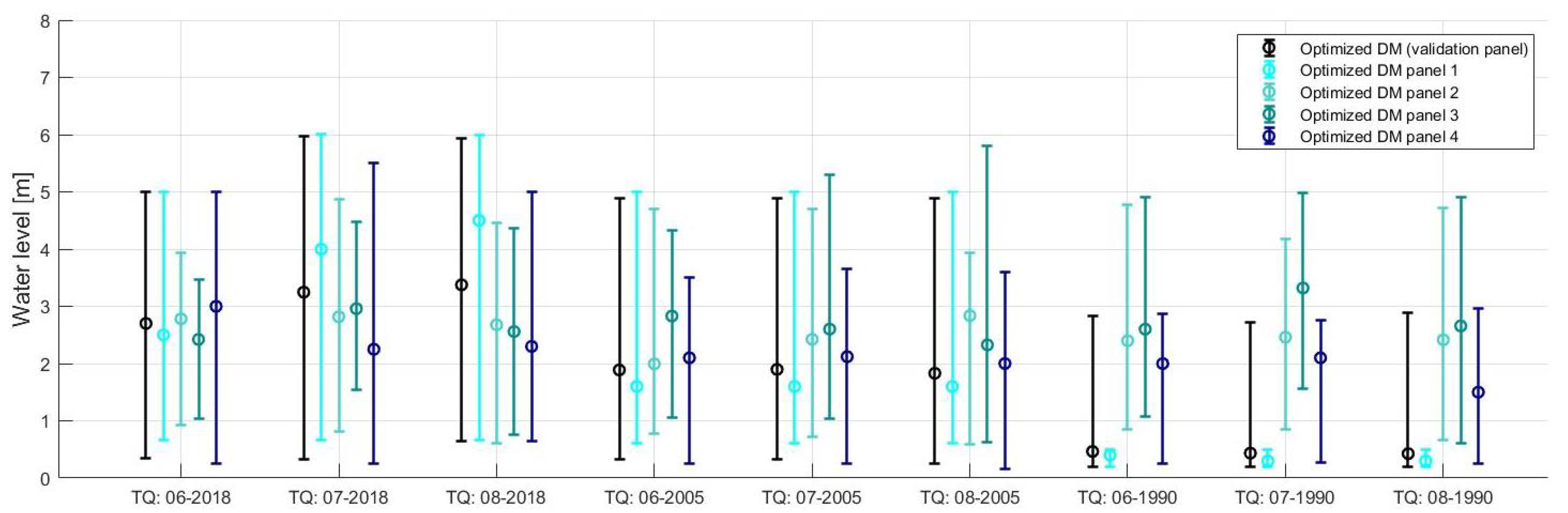
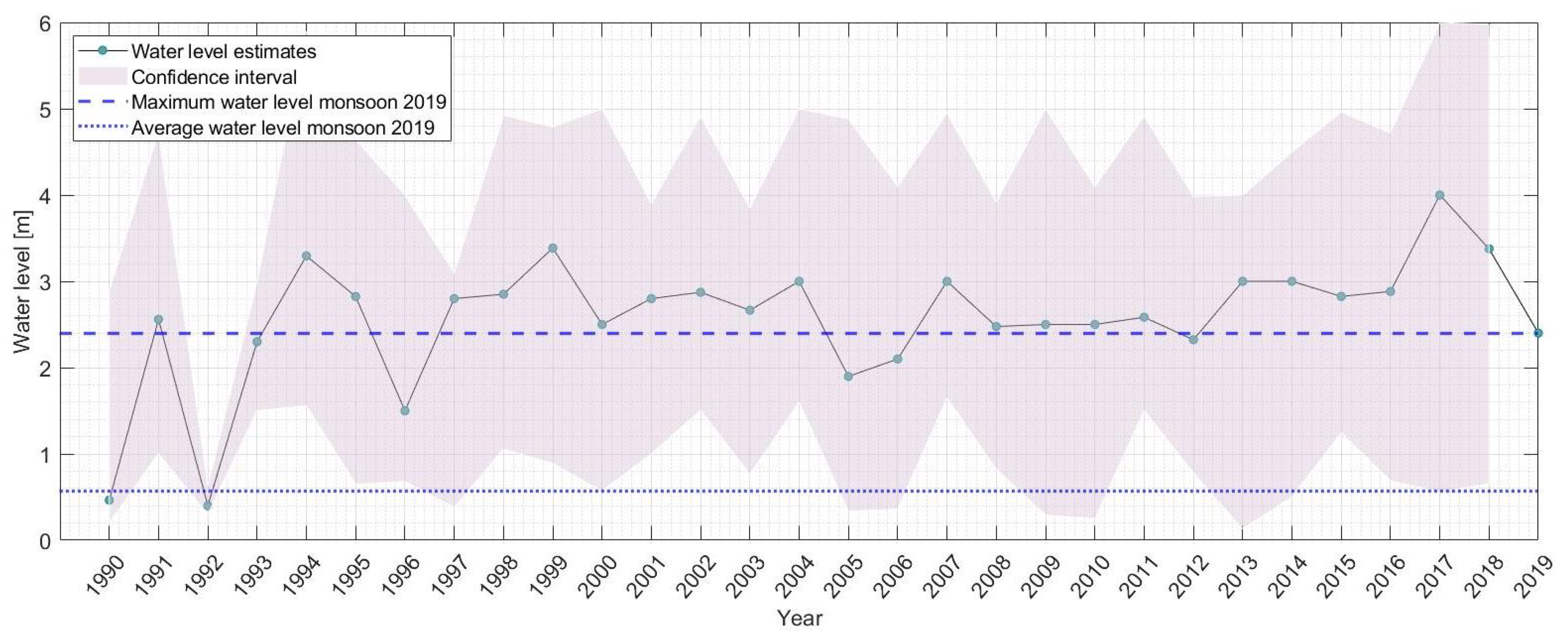
3.2. Maximum Water Levels

Combining the data of the different panels has resulted in monthly maximum water levels for the monsoon months for the years 1990–2019. Out of all 90 months, there were nine months, separated over three years, that were estimated by all 62 experts. For those months, we used the assessments of the optimized DM’s based on the validation panel. For the other months, the assessments of the optimized DM’s per panel were used. As mentioned before, to determine return levels, yearly maximum water levels are preferred. These were determined as the maximum of the three monsoon months of a year. The results are presented in Figure 5. The estimates of the water levels are the optimized global weight DM’s 50% quantile estimates. To emphasize the large uncertainties of the resulting DM’s assessments, the 90% confidence intervals are provided by the resulting 5% and 95% quantiles. The maximum water level of 2019 was not obtained from SEJ, since water level measurements of S4W were available for the monsoon of 2019.

According to the results of the SEJ analysis (Figure 5), the mean maximum water level for 1990–2019 is 2.57 m. The highest maximum water level was 4.0 m and occurred in 2017. The lowest maximum water level was 0.4 m and occurred in 1992. To get an idea of the orders of magnitude and deviation, we added the values of the maximum water level (striped line) and the average water level (dotted line) of the monsoon 2019.

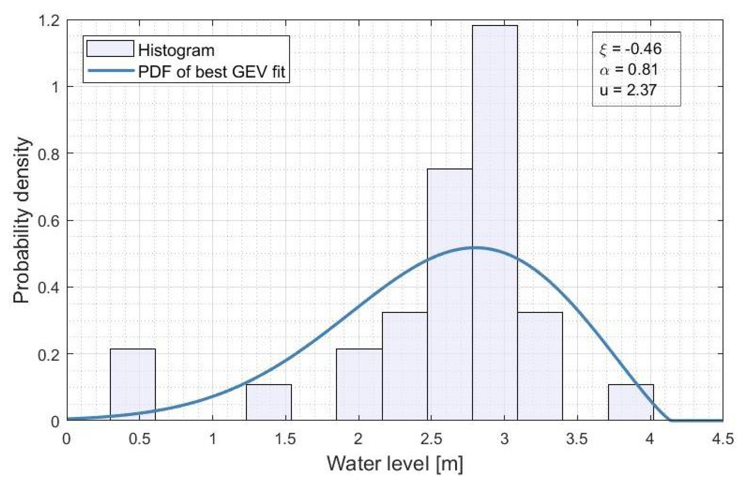
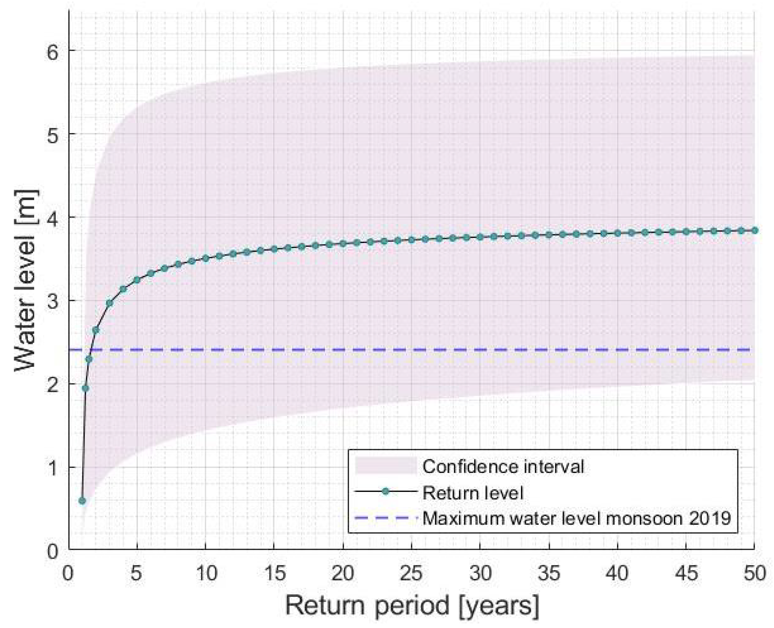
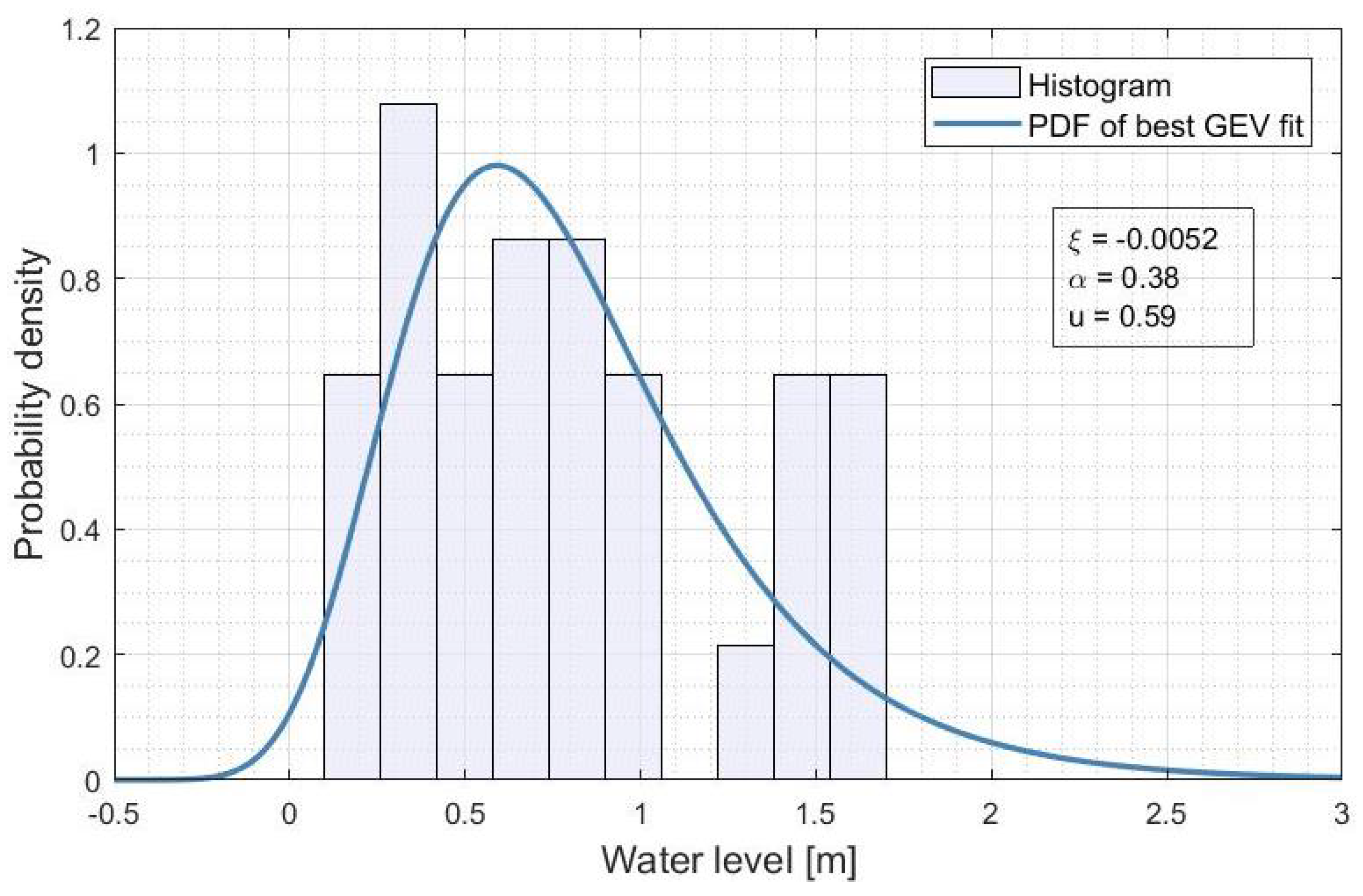
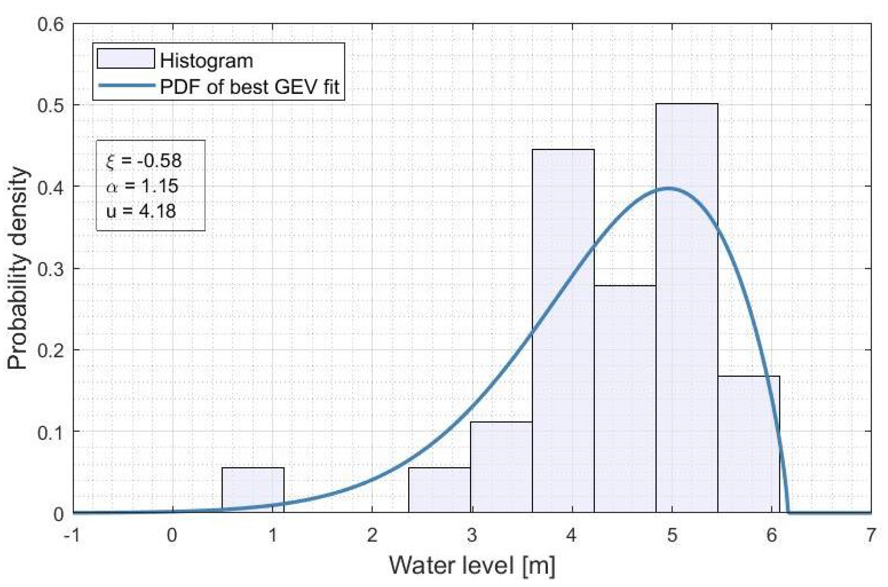
3.3. Return Level Analysis

With the constructed time series, it is possible to fit a GEV distribution to the resulting yearly maxima. This time series of the yearly water levels, as shown in Figure 5, shows more data points above the average than below. As a result, the histogram is negatively skewed (i.e., has a tail on the left hand side and the peak is more on the right hand side), which is surprising. In general, a histogram of maximum water levels has a tail on the right hand side [28]. The resulting shape obviously suggests a negatively skewed distribution, which is the shape of the probability density function (PDF) of a type III (Reverse Weibull) extreme value distribution. Consequently, also MATLAB suggested a Reverse Weibull (type III) as best-fitting GEV, as shown in Figure 6, which includes the estimated parameters. The numerical value of the shape parameter $\xi$ is negative (−0.455), implying the type III extreme value distribution. The estimated location parameter is 2.37 and the estimated scale parameters is 0.81.

To obtain confidence intervals for the return levels, we fitted a GEV distribution for the 5% and 95% quantile estimates of the water levels. The best-fitting GEV distributions along with and their corresponding estimated parameter are presented in Appendix C. The fitted distributions are not the same. For the lower bound (5%-quantile), the maxima data are best fitted by a Gumbel distribution ($\xi$ = 0) which differs from the reverse Weibull obtained for the 50%-quantile. The 95%-quantile yield dat is best fitted by a reverse Weibull distribution.

By taking the inverse of the fitted GEVs, we calculated the return periods corresponding to the extreme water levels, including the confidence intervals, as shown in Figure 7. The dots represent the resulting return levels, whereas the 90% confidence interval is depicted by the shaded area.

The confidence interval is wide, which originates from the large uncertainty inherited by the DM’s. We found that a water level of $3.25\pm 2$ m has a return period of five years. A water level of $3.51\pm 2.1$ m has a return period of ten years and finally, a water level of $3.84\pm 2$ m would statistically occur once every fifty years.

4. Discussion

A remarkable observation of our analysis is that specialists’ assessments did not necessarily perform better than citizens’ assessments. In fact, the two experts that the optimized DM of the combined panel relied on, were both citizens of Bhaktapur. A possible explanation could be that specialists tend to be more certain and hence overconfident about their assessments. A comparison of experts’ calibration score and information score with respect to domain expertise is graphically depicted in Figure A1 in Appendix B. It is visible that the highest 11 calibration scores are held by non-specialists, including the calibration scores higher than the 0.05 significance level. Nonetheless, there are many non-specialists with very low calibration, so an overall comparison between the two groups is inopportune.

By using SEJ, we were able to reconstruct unavailable historical water levels for the Hanumante River (see Figure 5). Due to the lack of data, the accuracy of the reconstructed water levels and corresponding return periods are therefore hard to validate. A possible validation approach is to use the available precipitation data from DHM. Nonetheless, the precipitation-discharge relation and stage-discharge relation are not known, which hampers this validation approach. This conclusion is also reached when comparing the precipitation data from DHM to the reconstructed water levels, as no direct relation between the two sets of observations can be observed. Nevertheless, we know that floods occurred 2015 and 2018 [1]. Looking at Figure 5, the highest estimated maximum water level occurred in 2017 and was 4.0 m, while the years for which higher water levels were expected did not exhibit higher water levels. This implies that the SEJ water level estimates are not consistent with the two available observations for the water level maximum. Nevertheless, this is not necessarily a problem for the purpose of this study.

A strong aspect of this study is that there is evidence that the order of magnitude of the estimated water levels is correct. The maximum water level measured in the Hanumante River by S4W-Nepal during the 2019 monsoon was 2.4 m. With respect to the water levels obtained from SEJ, this value is comparable to the average of the water levels between 1990 and 2018, which equals 2.57 m. This is also in line with our expectations, since the monsoon of 2019 was an average monsoon, based on the expertise of S4W researchers. From this, we conclude that the order of magnitude of the yearly water levels obtained with SEJ can be regarded as accurate.

It is important to mention that the main objective of this research is not to reproduce the exact values of extreme water levels and match it to the correct year, but to obtain the frequency of the extreme water levels. Validation of the return periods is therefore still essential. The return periods of the water levels were validated with available information. The Siddhi Memorial Hospital is very close to the location under consideration and is situated at about 3.4 m (based on levelling measurements). The results of the return level analysis imply that the hospital would be flooded every $\pm 7$ years. From interviews with the hospital employees, it turned out that the hospital indeed faced multiple floods in the last 30 years with a major event in 2015 [29]. This leads to the conclusion that the frequency of the water levels resulting from the reconstructed time series is credible.

Concluding, given the lack of data for extreme water levels, the range of values and the frequency of the water levels do provide us useful information, especially when taking into account the uncertainty. In situations like this, where little data exist, SEJ is the best available methodology available. Should there had been any data available, no SEJ would have been needed.

Apart from this main insight, there are some other interesting aspects to address. Firstly we saw that, although the selected experts for the DM’s had difficulties in remembering water levels of specific years, there were also experts who did remember the extreme events of 2015 and 2018, as became clear during conversations. They might have been excluded in the DM due to their low calibration scores, which denoted low statistical accuracy for the calibration questions. This shows that informative assessments for certain questions of interest get lost if the performance for the calibration questions is poor. However, we note that a comparable risk exists with measured data: it can happen that water levels are measured right before an extreme rainfall event, meaning that the maximum water level of that day is missed.

Furthermore, due to the lack of available data, we had to include two calibration questions (CQ1 and CQ2) about other rivers in the region than the Hanumante river. This might be a limitation to the study, because these questions had no direct connection with the questions of interest. However, when looking at Figure 3, it can be concluded that the experts did not necessarily perform worse for these questions.

Investigating performance over calibration questions, we notice that for calibration questions 4 and 10, the performance has been poor in most of the panels. It is remarkable that both questions were about June 2019. The groups overestimate the water levels for these questions, since both measured values are relatively low. It is possible that the ’real’ maximum water level of June 2019 was higher but that it has not been measured, since the water level is only measured once a day (from monsoon 2019 onward).

Considering the questionnaire, it was observed that experts took a relatively long time to complete it. The average duration of a questionnaire turned out to be around thirty minutes and some of the experts could not bring up the time and effort to give thoughtful responses until the final question. Consequently, the answers for the final years, say 1995 till 1990, did not show a lot of variation. People started repeating their assessments for these consecutive years, also because they could not remember the water levels of these specific years well. It would have been more sensible to not overwhelm the experts with such a vast questionnaire, but instead make an appointment with them to have more time to discuss the implications of the research and the importance of their recollections of the extreme water levels.

Additionally, several experts seemed to struggle with the interpretation of the confidence intervals and translation was an important issue. We relied a lot on our S4W colleagues as interpreters, since it was sometimes impossible for us to directly communicate with the experts. These comment applies especially for the experts from the category ’Citizens of Bhaktapur’, who mostly answered the questionnaire during their working hours.

Also the resulting histogram of the water levels, as mentioned in Section 3.3, is rather surprising, leading to an unexpected best-fitting GEV distribution. The main reason for this is the fact that the analysis is based on 30 data points (1990–2019), which is a very small amount. More data could lead to a different best-fit GEV and therefore a different return level graph.

Regarding the return level graph, it should be noted that it excludes any physical boundary conditions of the river, which influence the water levels especially when they exceed the river bank level and enter the flood plains. These aspects should be included to obtain more accurate estimations of the return levels.

After conducting this research, we suggest that the method definitely has potential, but that there are several opportunities to improve the application for a SEJ in a situation with few possibility to obtain data and few experts in the field. We would therefore recommend to consider the following aspects for any future research including SEJ:

• The experts should be better prepared for the questionnaires. An elaborate (oral) explanation of the method is extremely important. Especially the importance of the confidence intervals should be well explained. Moreover, it is advisable to provide the experts with even more background information. It would be useful to give the value of one recent monthly maximum water level. The experts could use this value to refer months of the past to a month that they remember and to understand how much the maximum can deviate from the median.
• It could be useful to ask the experts to start by estimating the water levels of months in which they remember that a flood or very high water level occurred. In this way, it is avoided that experts oversee to assess those years with relatively high values while they are working themselves trough the long list of years. Of course, it cannot be avoided that experts might just forget flood events of the past.
• It is important to choose the calibration questions thoroughly. If possible, all calibration questions should be related to the location of interest. If this is not possible, the locations should be close to the location of interest and the experts should be familiar with them. Besides, it is important that the behaviour of the variable of interest is similar at the other locations. So, the mean and maximum water levels should be comparable at the different locations.

Next to an improvement of the application of the SEJ method, we would recommend further research concerning the flood risk of the Hanumante River. Further research could include the following aspects:

• It would be useful to find a way to validate the results of the SEJ with precipitation data. In order to do so, it is necessary to obtain more knowledge about the relation between precipitation, discharge and water level for the Hanumante River. Furthermore, validation by data time series only makes sense when the reconstructed water levels match to the correct years. We think that validation with precipitation data has potential when our recommendations for application of SEJ are followed.
• We would recommend to continue on evaluating the flood risk by the Hanumante River. Further research could be done on the expected damages due to floods or about the possibilities to reduce damages by floods. The damages can be reduced by a proper evacuation plan. The application of a Community-Based Early Warning System (CBEWS) can play a major role for this. [30].
• Probably our most important recommendation is to highlight the importance of continuing actual water level and discharge measurements in the Hanumante River, if possible on a daily basis. Over time, these efforts would provide the much needed data that would ultimately improve our understanding of the return levels.

5. Conclusions

We have shown that it is possible to use estimates from both citizens and specialists to fill historical data gaps of water levels in the Hanumante River using SEJ return level analysis. The method has potential, especially with the lessons and recommendations of this research in mind. Within the chosen method of SEJ, it is important to select the calibration questions thoroughly and caution should be exercised in the explanation and translation (when needed) of the method and the questionnaire. It is extremely important that the experts fully understand the method and the questions.

A very interesting conclusion of this research is that water specialists did not necessarily provide better performing assessments than citizens. Being familiar with the river seemed to be more important than the knowledge about flood risk. This conclusion may trigger a wider horizon of possible experts for similar studies as well. It is important to realize that citizens can possess valuable knowledge as well, especially in regions were ‘real’ experts are scarce.

Experts were not able to accurately remember water levels of specific years, but they did remember the order of magnitude. As long as the large uncertainty is taken into account and the obtained return levels are only used to indicate the order of magnitude of occurring water levels, the reconstructed water levels of Hanumante River, based on SEJ, can be used for a return level analysis. This statement is confirmed by the correct order of magnitude of the return levels.

References

1. Prajapati, R.; Raj Thapa, B.; Talchabhadel, R. What flooded Bhaktapur? My Republica, 17 July 2018. [Google Scholar]
2. Davids, J.C. Mobilizing Young Researchers, Citizen Scientists and Mobile Technology to Close Water Data Gaps. Ph.D. Thesis, Delft University of Technology, Delft, The Netherlands, 2019. [Google Scholar]
3. Central Bureau of Statistics. National Population and Housing Census 2011; Technical Report 7; Government of Nepal, National Planning Commission Secretariat: Kathmandu, Nepal, 2012.
4. ICIMOD. Land Cover Distribution for Bhaktapur; ICIMOD: Khumaltar Kathmandu Khumaltar, Nepal, 2010. [Google Scholar]
5. Bhatta, B.P.; Pandey, R.K. Bhaktapur Urban Flood related Disaster Risk and Strategy after 2018. J. APF Command Staff Coll. 2020, 3, 72–89. [Google Scholar] [CrossRef]
6. Pradhan-Salike, I.; Pokharel, J.R. Impact of Urbanization and Climate Change on Urban Flooding: A case of the Kathmandu Valley. J. Nat. Resour. Dev. 2017, 7, 56–66. [Google Scholar] [CrossRef] [Green Version]
7. Department of Water Induced Disaster Prevention. Preparation of Flood Risk and Vulnerability Map Final Report; Technical Report; Government of Nepal, Ministry of Water Resources: Lalitpur, Nepal, 2009.
8. Smartphones4Water. Projects S4W-Nepal. Available online: https://www.smartphones4water.org/projects/nepal/ (accessed on 16 October 2019).
9. Cooke, R.M. Experts in Uncertainty, Opinion and Subjective Probability in Science; Oxford University Press: Oxford, UK, 1991. [Google Scholar]
10. Cooke, R.M.; Goossens, L.L. TU Delft expert judgment data base. Reliab. Eng. Syst. Saf. 2008, 93, 657–674. [Google Scholar] [CrossRef]
11. Colson, A.R.; Cooke, R.M. Cross validation for the classical model of structured expert judgment. Reliab. Eng. Syst. Saf. 2017, 163, 109–120. [Google Scholar] [CrossRef] [Green Version]
12. Cooke, R.M. Special issue on expert judgement. Reliab. Eng. Syst. Saf. 2008, 93, 655–656. [Google Scholar] [CrossRef]
13. Hathout, M.; Vuillet, M.; Peyras, L.; Carvajal, C.; Diab, Y. Uncertainty and expert assessment for supporting evaluation of levees safety. In Proceedings of the 3rd European Conference on Flood Risk Management FLOODrisk Oct 2016, Lyon, France, 17–21 October 2016. [Google Scholar] [CrossRef] [Green Version]
14. Cooke, R.M.; Slijkhuis, K.A. Expert judgment in the uncertainty analysis of dike ring failure frequency. Case Stud. Reliab. Maint. 2003, 480, 331. [Google Scholar]
15. Sjöstrand, K.; Lindhe, A.; Söderqvist, T.; Rosén, L. Water Supply Delivery Failures—A Scenario-Based Approach to Assess Economic Losses and Risk Reduction Options. Water 2020, 12, 1746. [Google Scholar] [CrossRef]
16. Burgman, M.A.; McBride, M.; Ashton, R.; Speirs-Bridge, A.; Flander, L.; Wintle, B.; Fidler, F.; Rumpff, L.; Twardy, C. Expert status and performance. PLoS ONE 2011, 6, e22998. [Google Scholar] [CrossRef] [PubMed]
17. Page, S.E. The Difference: How the Power of Diversity Creates Better Groups, Firms, Schools, and Societies-New Edition; Princeton University Press: Princeton, NJ, USA, 2008. [Google Scholar]
18. Ungar, L.; Mellers, B.; Satopää, V.; Tetlock, P.; Baron, J. The good judgment project: A large scale test of different methods of combining expert predictions. In Proceedings of the 2012 AAAI Fall Symposium Series, Arlington, TX, USA, 2–4 November 2012. [Google Scholar]
19. Tetlock, P.E.; Gardner, D. Superforecasting: The Art and Science of Prediction; Random House Books: Manhattan, NY, USA, 2016. [Google Scholar]
20. Schumann, G.J.P.; Neal, J.C.; Mason, D.C.; Bates, P.D. The accuracy of sequential aerial photography and SAR data for observing urban flood dynamics, a case study of the UK summer 2007 floods. Remote Sens. Environ. 2011, 115, 2536–2546. [Google Scholar] [CrossRef]
21. Carpenter, L.; Stone, J.; Griffin, C.R. Accuracy of aerial photography for locating seasonal (vernal) pools in Massachusetts. Wetlands 2011, 31, 573–581. [Google Scholar] [CrossRef]
22. Sada, R. Hanumante River: Emerging uses, competition and implications. J. Sci. Eng. 2012, 1, 17–24. [Google Scholar] [CrossRef]
23. Wittmann, M.E.; Cooke, R.M.; Rothlisberger, J.D.; Lodge, D.M. Using Structured Expert Judgment to Assess Invasive Species Prevention: Asian Carp and the Mississippi—Great Lakes Hydrologic Connection. Environ. Sci. Technol. 2014, 48, 2150–2156. [Google Scholar] [CrossRef] [PubMed]
24. Leontaris, G.; Morales-Nápoles, O. ANDURIL—A MATLAB toolbox for ANalysis and Decisions with UnceRtaInty: Learning from expert judgments. SoftwareX 2018, 7, 313–317. [Google Scholar] [CrossRef]
25. Bali, T.G. The generalized extreme value distribution. Econ. Lett. 2003, 79, 423–427. [Google Scholar] [CrossRef]
26. De Haan, L.; Ferreira, A.F. Extreme Value Theory: An Introduction; Springer: New York, NY, USA, 2006; pp. 3–36. [Google Scholar]
27. VNK. The National Flood Risk Analysis for the Netherlands; Technical Report; Rijkswaterstaat: Utrecht, The Netherlands, 2014. [Google Scholar]
28. Soomere, T.; Eelsalu, M.; Pindsoo, K. Variations in parameters of extreme value distributions of water level along the eastern Baltic Sea coast. Estuar. Coast. Shelf Sci. 2018, 215, 59–68. [Google Scholar] [CrossRef]
29. Ojha, A. Bhaktapur settlements submerged. Kathmandu Post, 28 August 2015. [Google Scholar]
30. Smith, P.J.; Brown, S.; Dugar, S. Community-based early warning systems for flood risk mitigation in Nepal. Nat. Hazards Earth Syst. Sci. 2017, 17, 423–437. [Google Scholar] [CrossRef] [Green Version]
Figure 1. Overview of the Kathmandu Valley and Bhaktapur. HM04 and HM06 have been used in the calibration questions.
Water 12 03229 g001
Figure 2. A comparison between scores of the optimized DM’s of the different panels.
Water 12 03229 g002
Figure 3. A comparison of the optimized Decision Makers of the different panels. The circles indicate the median estimate given by the optimized DM. The 5% and 95% quantiles are also given.
Water 12 03229 g003
Figure 4. A comparison of the optimized Decision Makers of the different panels based on the 9 overlapping target questions. The circles indicate the final estimate given by the optimized DM. The 5% and 95% quantiles are also given.
Water 12 03229 g004
Figure 5. Maximum water levels obtained with SEJ for 1990–2019 (dots), with 5% and 95% quantile estimates (shaded). The maximum water level (striped line) and the average water level (dotted line) of the 2019 monsoon are also added to get an idea of the orders of magnitude.
Water 12 03229 g005
Figure 6. The histogram of yearly maximum water levels and the probability density function of the fitted reverse Weibull distribution.
Water 12 03229 g006
Figure 7. Return periods for the water levels at the Hanumante River (dots), together with the 90% confidence interval resulted from DM’s 5% and 95% quantiles (shaded).
Water 12 03229 g007