Identifying the Influence of Land Cover and Human Population on Chlorophyll a Concentrations Using a Pseudo-Watershed Analytical Framework

Abstract

Increasing agricultural development and urbanization exacerbates the degradation of water quality in vulnerable freshwater systems around the world. Advances in remote sensing and greater availability of open-access data provides a valuable resource for monitoring water quality but harmonizing between databases remains a challenge. Here, we: (i) developed a pseudo-watershed analytical framework to associate freshwater lakes with adjacent land cover and human population data and (ii) applied the framework to quantify the relative influence of land cover and human population on primary production for 9313 lakes from 72 countries. We found that land cover and human population explained 30.2% of the variation in chlorophyll a concentrations worldwide. Chlorophyll a concentrations were highest in regions with higher agricultural activities and human populations. While anthropogenic land cover categories equated to only 4 of the 18 categories, they accounted for 41.5% of the relative explained variation. Applying our pseudo-watershed analytical framework allowed us to quantify the importance of land cover and human population on chlorophyll concentration for over 9000 lakes. However, this framework has broader applicability for any study or monitoring program that requires quantification of lake watersheds.

1. Introduction

Freshwater is essential for human life and provides habitat to over 10% of all species on earth [1]. While freshwater lakes are distributed around the world, accessible freshwater is finite and comprises less than 1% of all water on the planet and is facing degradation [2]. Chlorophyll is a commonly used proxy for primary production and is used globally as a measure of lake trophic status and water quality [3]. Factors influencing chlorophyll concentrations include nutrient inputs [4,5], climate [6] and human influences [7]. Nitrogen and phosphorus are known drivers of chlorophyll [5,8] and are commonly found in excess in runoff from urban and agricultural landscapes [9,10]. Further, climate-related drivers such as warm air temperatures and low wind speeds can increase the stability of stratification in the water column which can result in increased algal biomasses [11]. Increases in the global human population and land-cover changes have also negatively affected freshwater quality [12]. Increased agricultural demand [13] and urbanization [14,15] both have contributed to increased runoff into lakes. All types of land cover contribute nutrients from the watershed into waterways, although the amounts and types of nutrients that come from nonpoint sources depend on a variety of drivers that include weather, topography, soil properties, land characteristics and management practices [16,17]. Here, we focus on further understanding the role of land cover and human population on chlorophyll concentrations in lakes worldwide.

The UN estimates that 70% of the world population will live in urban areas by 2050 [18] Urbanized regions have increased impervious surfaces which have been linked to hydrological changes that degrade water quality [19,20]. Runoff and stormwaters from such regions contain higher sediment content, nutrients, heavy metals, oil and grease, pesticides and bacteria [21] which directly end up in aquatic systems [16]. In response to a growing population, a substantial expansion of agricultural production and water use will be needed in the coming decades to provide the necessary food and products to support the population growth and to replace agricultural lands lost to urban expansion [13,22] Agricultural land can impact water quality, such as through croplands [23] that are frequently sprayed with phosphorus rich pesticides [24] and administered nutrient rich fertilizers [25]. The inputs of nitrogen and phosphorus from nonpoint sources like fertilizers and pesticides can degrade water quality and have been associated with higher chlorophyll a concentrations in watersheds with agricultural land cover [26,27]. Pasturelands from raising livestock can also affect water quality through increased soil erosion [28,29]. Quantifying the cover of agriculture and urbanization within lake watersheds can help manage lake water quality.

Chlorophyll a concentrations can be elevated in watersheds with higher population density [30]. Such regions have multiple sources of nutrient inputs into freshwater lakes such as greater discharge of food, sewage, industrial waste and wastewater, which ends up loading freshwater bodies [4,31]. For example, human population density has been found as a driver of chlorophyll in the Laurentian Great Lakes [25]. Thus, understanding anthropogenic effects on lakes requires investigation into human population densities and urban land cover.

Although land cover and human population are known determinants of chlorophyll concentrations in lakes, we are currently limited by our ability to appropriately quantify the proportion of each land cover category and the number of people within a lake’s watershed. Advances in remote sensing and data availability provide an opportunity to harmonize land cover and human population data from disparate sources [32] in order to develop a broader understanding of the effects for lakes. A novel analytical framework was necessary for the creation of watersheds for lakes where the delineated watershed is not known, particularly for small and remote lakes. This framework allows lakes with known and unknown watersheds to be equally analyzed. Studies to date on the impacts of land cover and human population on primary production have been largely regional, examining the effects of these drivers within a single or few watersheds that have been previously delineated [27,33,34,35]. Using the proposed methodology for generating watersheds, we can analyze globally drivers of chlorophyll in lakes.

Our goal was to quantify the relative influence of land cover and human population on chlorophyll a concentrations for over 9000 freshwater lakes distributed across 72 countries and on every continent. First, we developed a novel analytical framework to quantify the proportion of each land cover category and the number of people living within a watershed. Second, we tested the analytical framework to quantify the influence of land cover and human density on chlorophyll a concentrations. We hypothesized that chlorophyll a concentrations would be higher in areas with larger human populations and a greater human footprint (i.e., more agriculture or urban areas) because of increased nutrient inflow from human activities. We expect that land cover and human population within the developed pseudo-watersheds will explain a significant portion of the variation in chlorophyll a concentrations.

2. Materials and Methods

2.1. Data Acquisition

We acquired chlorophyll a, water chemistry and lake morphology data from an online database of lakes distributed globally [36]. The database included 228,166 unique observations from 11,941 lakes [36]. Lakes were removed if their watersheds consisted of more than 50% water which could occur due to the lake being coastal or surrounded by other lakes. This reduced the number of lakes in this study to 9313, although 75% of these lakes were found in North America due to the increased availability of data. If data were collected for multiple years for a lake, the data from the most recent year was chosen, such that only spatial patterns were assessed. If data had more than one observation in a year, we selected the month with the highest concentration for chlorophyll a. Across the dataset, chlorophyll concentrations were expressed in mg/L.

Human population data were acquired from a NASA dataset called “Gridded population of the world” [37]. This dataset estimated the distribution of humans using population prediction in combination with census data and spatial density at a variety of spatial resolutions. We chose the best resolution available at 1 km [37]. Land cover data was acquired from NASA Earth Data and used Moderate Resolution Imaging Spectroradiometer (MODIS) to categorize land cover into 17 categories. The categories included 500 m × 500 m cells of a variety of land covers including forest, grasslands, wetlands, urban, agriculture, permanent snow, barren land and water [38]. We used the 2015 version of both the land cover and the human population data because 2015 provided the best balance between recency and accuracy with the sampling year of the studied lakes. In the dataset, land cover categories are presented as a proportion of the cells in the pseudo-watershed. Human population was expressed as the total number of people within the pseudo-watershed.

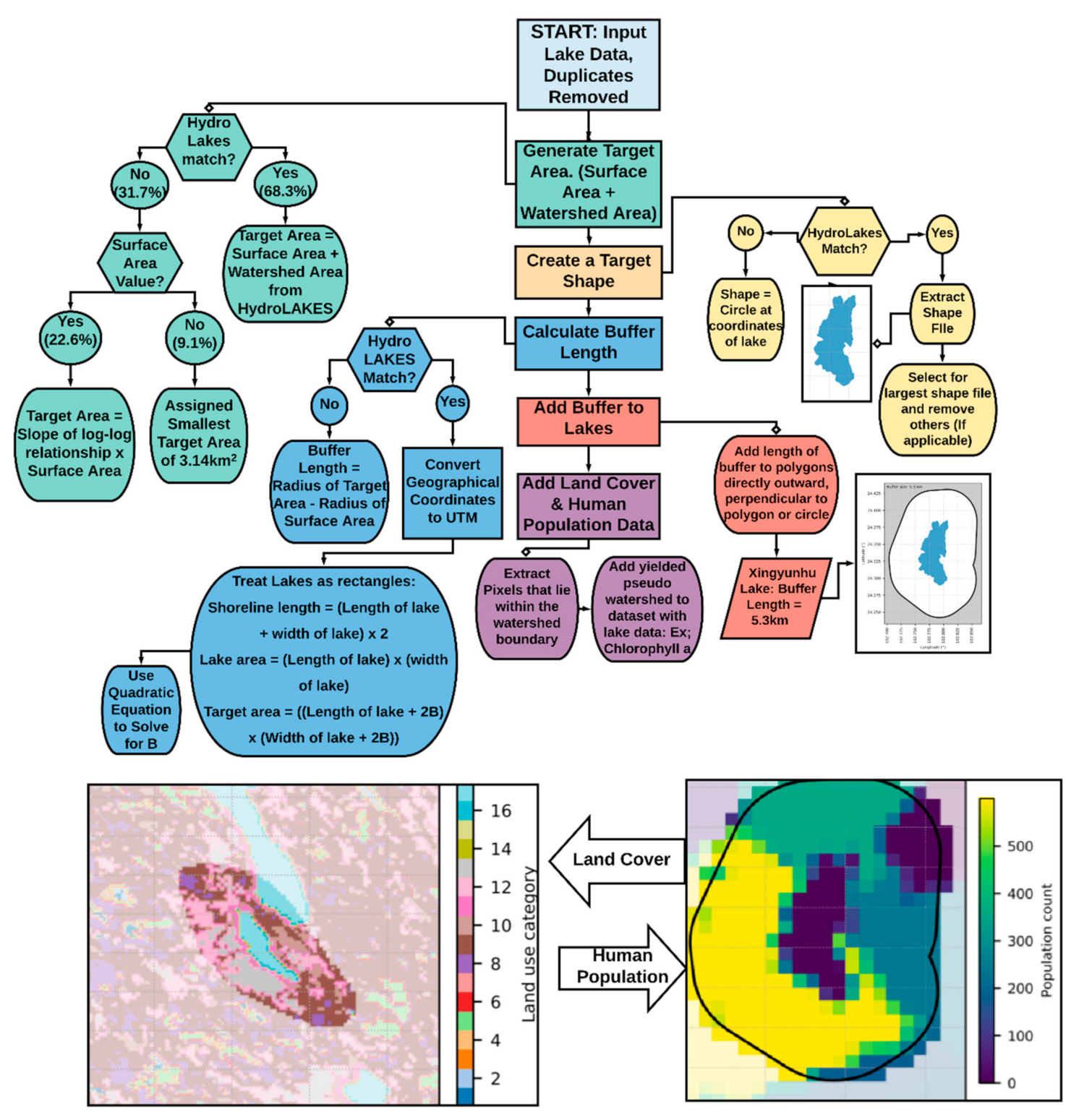
2.2. Development of an Analytical Framework

We developed a framework to estimate land cover and human population for the watershed surrounding a lake (Figure 1). This could be applied to the 1.4 million lakes larger than 10 ha for which shapefiles of shoreline polygons are readily accessible [39]. Open-access code to conduct this framework is available at: https://doi.org/10.5281/zenodo.4161959.

Step 1: Input Lake Data

We imported basic lake information that included lake name, latitude and longitude, chlorophyll a, and, where available, lake area. Our chlorophyll a database contains over 250,000 occurrences as there are many lakes with multi-site and/or multi-year entries [36]. We selected unique instances of lakes by their coordinates to ensure only one watershed is drawn for each lake. Chlorophyll a concentrations were also reviewed to avoid cases of multiple sampling coordinates within the same lake.

Step 2: Look for HydroLAKES match

We used the lake coordinates (lat,lon) and implemented the function find_hydrolakes_match to identify the nearest HydroLAKES polygon, as well as the distance from the sample coordinate to the edge of the HydroLAKES polygon. If the distance is 0 km (i.e., the sampling point is within the polygon), we called this a match, extracted the HydroLAKES polygon shapefile and recorded the corresponding lake area, watershed area and shoreline length. Finding a HydroLAKES match is the ideal situation as HydroLAKES provides easily accessible and readily available shoreline polygons, shoreline length, surface area, mean depth, volume and residence time for 1.4 million lakes [39]. In situations where there were no HydroLAKES matches, we used a surface area value from our original chlorophyll database to complete the creation of a pseudo-watershed. This was necessary for 22.6% of the lakes included in the analysis. [36].

Step 3: Generate Watershed Target Area

We used three methods to define a watershed target area (lake surface area + watershed area) around each lake based on the combined area of the surface of the lake and its watershed: (Case 1) Using the sum of surface area and watershed area values provided by HydroLAKES (68.3% of lakes), (Case 2) for lakes without a HydroLAKES match but with a surface area value (22.6% of lakes), we calculated the target area by using the slope of the log-log relationship between surface area and target area (i.e., surface area + watershed area) from the lakes within the HydroLAKES repository [39] (Case 3) if the lakes have neither a watershed area nor a surface area (9.1% of lakes), they are assigned the smallest target area which is a circle of radius 1 km and area 3.14 km². These lakes were assigned the smallest target area because HydroLAKES includes coverage of almost all large lakes and thus lakes without a match are likely too small to be identified by remote sensing or GIS methods.

Step 4: Create a target shape

Each lake has a unique shape that should be represented by an accurate shape or an estimation of its shape based on its surface area. We used two methods for creating a target shape depending on whether a shapefile existed from a HydroLAKES match. First, for lakes with a HydroLAKES match, the lake possessed a shapefile as part of the HydroLAKES repository that indicated the shape of the lake as a polygon [39]. The watershed was drawn as an “expansion” of this lake shape, equally in all directions, along the perimeter of the shape file of the lake to respect the shape of the lake. If there was more than one shapefile provided by HydroLAKES (likely from islands being present), we selected the primary and largest portion of the lake (i.e., the exterior perimeter). Second, if there was no HydroLAKES match, the final target shape is a circle with the theorized target area (“Case 2” in Step 3) centered on the sampled location coordinates in the lake. If the lake also had no value for surface area, a circle with the minimum target area of 3.14 km² was applied (“Case 3” in Step 3), this polygon was centered on the location of the sampled coordinates using the function Point(lat,lon).

Step 5: Convert geographic coordinates

We converted the geographical units from latitude-longitude to the Universal Transverse Mercator (UTM) in order to standardize the (horizontal and vertical) map units and solve for the size of the buffer of each watershed in meters.

Step 6: Calculate buffer size for HydroLAKES matches

To estimate the length of the watershed buffer value that will be applied equally and perpendicularly from the shoreline of the lake, we treated the lakes and watersheds as rectangles. From the lake’s shoreline length (extracted from the HydroLAKES database), the lake’s area and the target area, we determined an estimate of the buffer.

Shoreline length = (Length of lake + width of lake) × 2

Lake area = (Length of lake) × (width of lake)

Target area = ((Length of lake + 2buffer) × (Width of lake + 2buffer)).

This final quadratic equation was used to solve for the length of buffer. If the calculated buffer size was smaller than 1 km, it was adjusted to 1 km.

Step 7: Draw watersheds on lakes

After the buffer values were calculated and adjusted for accuracy, they could be applied to the lakes with a predefined shape. The polygons for all lakes were reduced to maximum 10 sides in order to reduce processing load, with the caveat that the area of polygons may be slightly larger or smaller than the original. The calculated buffer was added directly outward, perpendicular to the perimeter of the simplified polygon. This created an expanded polygon that includes the lake area with a distinct watershed area. The geographical reference frame was converted back to latitude-longitude.

Step 8: Adding corresponding land cover and human population data

Using the generated pseudo-watersheds, the land cover and human population data were extracted for each watershed. In this way, we could obtain a more realistic count of people within the watersheds and the proportion of each land cover category within the watershed. In the past, we would be limited to quantifying land cover or population estimates within a pre-defined buffer surrounding a lake without consideration of lake shape or watershed size.

Land cover and human population cells were added to the framework using our custom-built analytical framework provided. The pseudo-watershed polygon (or circle) was reprojected to the grids of the human population data and land cover data, extracting only pixels that lie within the boundary of the polygon. This yielded the number of pixels of each land cover category within each watershed buffer and the total human population within the watershed buffer.

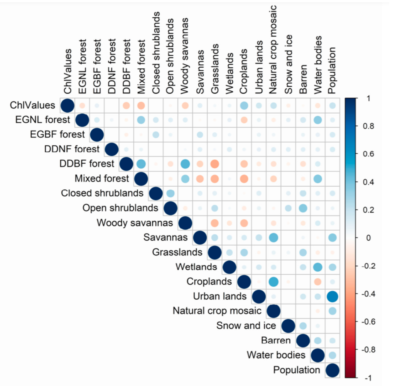
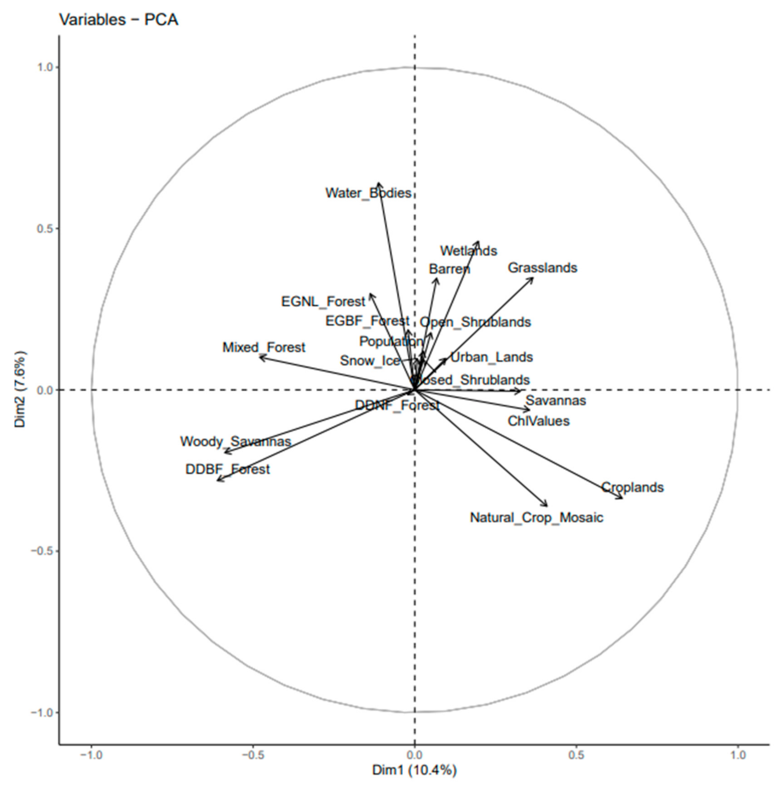
2.3. Statistical Analysis

We quantified the relationship of land cover and human population on chlorophyll using Spearman correlations, Principal Component Analysis and Random Forests. We assessed the normality of all variables using an Anderson-Darling normality test which revealed that chlorophyll was not normally distributed (p < 0.05). Log transformed chlorophyll concentrations were also not normally distributed but were used for this analysis. We quantified the correlation between the proportion within each pseudo-watershed for each land cover category and human population with chlorophyll a using Spearman correlations (cor.test) in R [40]. The Spearman correlation is a nonparametric test which measures the strength and direction of association between ranked variables [41].

We conducted a Principal Component Analysis (PCA) with function prcomp to assess the strength of the relationship between chlorophyll and the 17 categories of land cover [42]. Principal axes were generated to explain the maximal amount of variation in the data. The PCA algorithm generates principal components (axes) where the data shows the maximum amount of variation [43]. The PCA outputs a two-dimensional ordination plot which visualizes the relationships between predictor variables [43]. A broken stick analysis (Package PCDimension, [44]) and scree plot test were used to identify the three significant axes in the Principal Component Analysis. The PCA was visualized using the R function fviz_pca_var [42].

We conducted a random forest (Package: randomForest) to identify the hierarchical importance of land cover and human population variables on chlorophyll a concentrations [45]. The random forest used 500 regression trees to identify the level of importance of each of the land cover categories and human population. Random forests are built as ensembles of decision trees and work through bootstrap aggregation [46,47]. Subsets of data are randomly sampled upon which models are fit and it is based on these aggregated predictions that the best model is selected [46,48]. In this study chlorophyll is being tested against land cover and human populations (drivers) to identify which predictors individually explain the most variation.

3. Results

3.1. Analytical Framework for the Development of Pseudo-Watersheds

The chlorophyll concentrations were mapped to visualize the geographical distribution of the 9313 sampled lakes in this analysis (Figure 2). The dataset consists of 9313 lakes in 72 countries on all continents including Antarctica. However, the majority of lakes are located in the United States (8266 lakes).

Of the 9313 lakes, the analytical framework created 6361 watersheds that were guided by the shoreline polygon from HydroLAKES while the remaining 2952 lakes had a circular watershed. The average pseudo-watershed size was 1894.37 km². The largest watershed was for the Aswan Reservoir in Egypt, which was 2,755,957.97 km² in size, the large size is because of the Nile River. The largest pseudo-watershed in North America, where the majority of the lakes are located, is the Lake Winnipeg pseudo-watershed which measured 815,024.47 km². The smallest watersheds were 3.14 km² which were lakes that had neither a HydroLAKES nor a value for surface area (Case 3).

Inside the watersheds, the average pseudo-watershed was represented by all land cover categories. Woody savannas and croplands represented the largest average proportions of land cover occupying 18.4% and 18.1% of the average watershed, respectively. On the contrary, closed shrublands and deciduous needleleaf forests were the least present in the pseudo-watersheds representing only 0.02% and 0.05% of the average watershed, respectively. There were only 341 pseudo-watersheds that were completely uninhabited while the largest population was 254,200,944 inhabitants located within the pseudo-watershed of the Three Gorges Reservoir in China. The average pseudo-watershed was made up of 73.9% natural land cover and 26.1% anthropogenic land cover with 148,645 inhabitants.

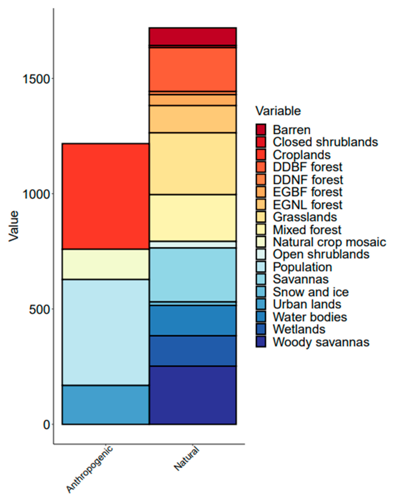
3.2. Quantification of Land Cover and Human Density on Chlorophyll Concentrations

Chlorophyll concentrations were higher in watersheds with more croplands (rho = 0.33, p < 0.0001), cropland mosaics (rho = 0.2, p < 0.0001) and people (rho = 0.2; p < 0.0001; Figure 3). Of the natural land cover categories, chlorophyll concentrations were slightly higher in grasslands (rho = 0.044, p < 0.0001) but lower in mixed forests (rho = −0.29, p < 0.0001), deciduous broadleaf forests (rho = −0.24, p < 0.0001) and woody savannas (rho = −0.22, p < 0.0001; Figure 3).

The broken stick model revealed that the PCA had 3 significant axes and explained 24.7% of the variation. The first principal component explained 10.4% of the variation and showed a positive association between proportion of savannas in a watershed and chlorophyll a concentrations and a negative relationship between chlorophyll a and the proportion of mixed forests in the watershed. The second principal component explained 7.6% of the variation and suggested chlorophyll a concentrations were positively associated with multiple land cover categories including, snow and ice, open and closed shrublands, as well as human population. Lastly, the third principal component explained 6.7% and suggested that chlorophyll a concentrations were higher in watersheds with a greater proportion of grasslands, urban lands and wetlands, while lower in watersheds with a higher proportion of deciduous broadleaf forests and woody savannas (Figure 4).

Land cover categories and total human population cumulatively explained 30.2% of the variation (mean of squared residual of 0.25) of chlorophyll a concentrations across 9313 lakes distributed worldwide. Of the predictors, croplands and total human population size within the watershed had the greatest influence on chlorophyll a, explaining 15.7% and 15.4% of the relative explained variation respectively (Figure 5). In total, anthropogenic variables—including the proportion of urban, cropland and cropland mosaic, in addition to human population—explained 41.5% of the relative variation of chlorophyll a concentrations. Of the natural land cover categories, grasslands and woody savannas were the next most important variables, explaining 9.1% and 8.8% of the variation respectively (Figure 5).

4. Discussion

4.1. Analytical Framework

We developed a pseudo-watershed analytical framework to quantify the influence of land cover and human population on chlorophyll a concentrations for 9313 lakes. Capitalizing on advances in remote sensing, GIS and in situ datasets, we provided a tool to harmonize disparate datasets to further understand lakes and their watersheds. Our analytical framework can be readily applied to lakes greater than 10 ha within the HydroLAKES database [39] to more realistically quantify land cover and human population within a lake’s watershed. This tool integrated data from a global chlorophyll a dataset, HydroLAKES, MODIS Land Cover and NASA Gridded Population of the World to create a workflow and framework with a variety of applications. Our analytical framework allowed us to capture 30% of the variation in chlorophyll a concentrations simply based on land cover and human population alone. The analytical framework we developed could address a variety of research questions that connect land cover, human population and other watershed characteristics to a number of freshwater response variables including water quality, contaminant levels, bacterial concentrations, fish populations and aquatic community composition [47]. We applied this analytical framework to showcase the importance of land cover and human population as significant drivers of chlorophyll a concentrations in freshwater lakes and emphasized the importance of mitigating nutrient inputs from agricultural and urban landscapes associated with human settlement.

The shape of a lake’s watershed is quite complex as it involves tracing all upstream inputs into a given lake. This detailed information is not readily available for most lakes on a global scale. With this in mind and with the goal of applying a consistent framework to 9313 lakes globally, we developed an approximation of the footprint of a lake’s watershed using a uniform (isotropic) enlargement of a polygon representation of the lake using HydroLAKES [39] or simply a circular representation for lakes less than 10 ha. By its nature, this isotropic enlargement results in the inclusion of not only upstream but also downstream areas; some upstream area is excluded at the expense of including downstream flows. When coupled with the MODIS land cover data and population data, this results in a bias for individual lake analyses. With 9313 lakes, it is anticipated that no bias exists. that is, populations are not biased to live either upstream or downstream of lakes globally, nor are forests, crops nor urbanized areas (land cover). For a random sampling of ~100 lakes, we visually confirmed the correct location of the pseudo watershed: MODIS land cover “water” classified pixels overlapped with the HydroLAKES lake polygon and the total population within the lake polygon was near or at zero.

4.2. Agricultural Influences on Chlorophyll

As expected, we found that chlorophyll a concentrations were higher in lakes whose watersheds have a higher proportion of agricultural activities. Anthropogenic land covers and human population were responsible for 41.5% of the relative explained variation in chlorophyll while representing only four of eighteen variables. We found that the proportion of croplands within a watershed was the most important driver of chlorophyll concentrations (rho = 0.33). The impact from cropland on chlorophyll a concentrations is mainly derived from the use of fertilizers used in agricultural practices which have led to a rise of nitrogen and phosphorus being added to the aquatic ecosystem [49]. The contribution of agriculture to eutrophication is caused by both current farming practices and the legacy of previous fertilizer use over the 20th century [50]. Crop uptake of nitrogen and phosphorus can be inefficient, resulting in overuse of fertilizer to ensure adequate growth rates [51]. Rain events cause the unused fertilizer to be washed away and deliver large quantities of nitrogen and phosphorus to lakes and other freshwater systems [52] For example, agricultural activities were responsible for 82% of nitrogen loading and 43% of phosphorus loading into freshwater lakes across Denmark [53]. Agriculture thus continues to be a significant driver of eutrophication in freshwater lakes globally.

Systematic land planning and modifications to nutrient application could allow for strong agricultural production coexisting with freshwater quality. Although cropland/natural vegetation mosaics were positively correlated with chlorophyll concentrations, the relationship was considerably weaker relative to cropland land cover. This suggests that mosaic landscapes might have less of an impact of chlorophyll because of the inclusion of more natural functions as a buffer to nutrient input [54] This indicates that strategic planning of agricultural land could alter mitigate negative effects water quality. A more conscious approach to fertilization could also mitigate the amount of nutrient loaded runoff that is currently contributing to higher chlorophyll concentrations [51].

4.3. Natural and Anthropogenic Land Cover

Watersheds with high chlorophyll a concentrations were typically had higher human populations (rho = 0.2) and more urbanized landscapes (rho = 0.17). High population densities around freshwater bodies are connected to modification in land cover and such changes result in wastewaters, stormwaters and runoff having increased nutrients [55,56]. Higher nutrient runoff is a particular concern in highly urbanized locations [57,58]. For example, Dianchi Lake is one of the most eutrophic lakes in China and its watershed is located near an urban area which received 240 million liters of runoff in 2000 [55]. As watersheds become more urbanized and their population grows, the number of human activities that degrade freshwater quality rises, for example, see Reference [8]. Moore et al. (2001) surveyed 30 lakes in Washington state and found that lakes located near urban areas were more likely to receive nutrient loading from wastewater and have higher values for chlorophyll as compared to lakes in undeveloped areas [33].

Increasing the level of vegetation within urban land cover offers the opportunity to improve the absorption of nutrients while reducing the amount of impervious surfaces in the landscape. The result is a decline in the overall volume of runoff that reaches freshwater systems [59]. The implementation of green infrastructure, such as stormwater ponds or green roofs, in urban landscapes can reduce nutrient loading into freshwater systems [60,61] while providing a co-benefit for natural systems [62]. Additionally, a reduction of wastewater discharge and an improvement in the treatment of wastewater offers an opportunity for both cities and citizens to reduce their impact on freshwater. Continued improvement of the process and standard of wastewater treatment is a key step in reducing point source nutrient loading from urban areas.

We found that forested landscapes were negatively associated with chlorophyll a concentrations (Mixed Forest rho= −0.029, Deciduous Broadleaf Forest rho = −0.24) and appeared to be essential in limiting the amount of runoff that is bound for freshwater systems [63]. In forested landscapes, soil is more porous and prone to water infiltration which reduces surface runoff and increases nutrient uptake [64]. Forested landscapes have the opposite effect of agricultural landscapes by reducing the inputs of total nitrogen and total phosphorus into lakes [50]. As such, maintaining undisturbed forests is key for mitigation efforts because activities such as logging and deforestation result in large scale modifications to the surrounding ecosystem and watershed [65].

4.4. Sustainable Water Management

The sustainability of water quality continually faces threats. The needs of the future must be considered equally with the demands of today for water resources to be truly sustainable [66]. In order to provide freshwater for all ecological and human requirements, availability, quality and access of freshwater must all be maintained to support its ecosystem services [67], including habitat, drinking water, nutrient cycling and recreation [68]. Activities within watershed are an important driver of water quality. For example, anthropogenic land cover has had a significant impact on the earth systems including freshwater [69,70]. Based on our results, watersheds with urban and agricultural land cover along with a high human population are linked to elevated chlorophyll concentrations and overall eutrophication of lakes. The sustainability of water resources is threatened by increased water demands and high volumes of wastewater [8,55] from urbanized regions and the addition of nutrient rich runoff from agriculture [49,53]. A large human population increases pressure on agriculture and other ecosystem services and also creates strain on the freshwater sustainability of that region [69]. Understanding the potential threats of degraded freshwater at the watershed scale is integral to the protection of water and ensuring it remains safe and accessible for today and the future for both ecological and anthropogenic needs.

4.5. Conclusions and Future Directions

Agricultural watersheds and human populations are established drivers of chlorophyll a concentrations, which can also influence phosphorus and nitrogen inputs [51]. Anthropogenic nutrient loading in combination with warming air and water temperatures, increased solar radiation and a stable water column can cause blooms of harmful cyanobacteria [71]. The effects of eutrophication and harmful algal blooms can go beyond effects on natural systems by impacting drinking water, tourism and real estate [72]. Managing chlorophyll concentrations is essential to maintaining the health of aquatic and terrestrial ecosystems while supporting public safety.

Based on their landscape position, lakes are supplied with nutrient rich runoff, wastewater and pollutants that are delivered by river network or overland drainage from anywhere in the watershed [73]. We identified that the land cover in watersheds has a strong effect on lake water quality. These findings suggest that conservation efforts for freshwater quality must extend beyond the lake to the watershed scale [21,27]. In regions where cropland is established as a significant portion of the watershed, we recommend: (i) limiting the excessive use of fertilizers [74]; (ii) increasing the efficiency of the water usage to reduce the amount of runoff [75]; (iii) creating natural buffers between agricultural fields and waterways to reduce potential nutrient runoff [76]; and (iv) increasing the proportion of natural land covers that reduce chlorophyll concentrations through land conservation or restoration. Mitigating nutrient inputs from agricultural and urbanized landscapes will be essential to preserving water quality and the essential ecosystem services freshwater provides [4]. Lastly, our study developed a novel analytical framework to connect remote sensing with in-situ data to further understand the relationships between freshwaters and their watersheds. We highlighted the importance of land cover and human population as significant drivers of chlorophyll concentrations in lakes across the world.

References

1. Reid, A.J.; Carlson, A.K.; Creed, I.F.; Eliason, E.J.; Gell, P.A.; Johnson, P.T.J.; Kidd, K.A.; MacCormack, T.J.; Olden, J.D.; Ormerod, S.J.; et al. Emerging threats and persistent conservation challenges for freshwater biodiversity. Biol. Rev. 2019, 94, 849–873. [Google Scholar] [CrossRef] [PubMed] [Green Version]
2. Strayer, D.L.; Dudgeon, D. Freshwater biodiversity conservation: Recent progress and future challenges. J. N. Am. Benthol. Soc. 2010, 29, 344–358. [Google Scholar] [CrossRef] [Green Version]
3. Carlson, R.E. A trophic state index for lakes. Limnol. Oceanogr. 1977, 22, 361–369. [Google Scholar] [CrossRef] [Green Version]
4. Carpenter, S.R.; Stanley, E.H.; Vander Zanden, M.J. State of the World’s Freshwater Ecosystems: Physical Chemical and Biological Changes. Annu. Rev. Environ. Resour. 2011, 36, 75–99. [Google Scholar] [CrossRef] [Green Version]
5. Quinlan, R.; Filazzola, A.; Mahdiyan, O.; Shuvo, A.; Blagrave, K.; Ewins, C.; Moslenko, L.; Gray, D.K.; O’Reilly, C.M.; Sharma, S. Relationship of total phosphorus and chlorophyll in lakes worldwide. Limnol. Oceanogr. 2020. [Google Scholar] [CrossRef]
6. Ward, N.K.; Steele, B.G.; Weathers, K.C.; Cottingham, K.L.; Ewing, H.A.; Hanson, P.C.; Carey, C.C. Differential Responses of Maximum Versus Median Chlorophyll-a to Air Temperature and Nutrient Loads in an Oligotrophic Lake Over 31 Years. Water Resour. Res. 2020, 56, e2020WR027296. [Google Scholar] [CrossRef]
7. Theissen, K.M.; Hobbs, W.H.; Ramstack, J.M.; Zimmer, K.D.; Domine, L.M.; Cotner, J.B.; Sugita, S. The altered ecology of Lake Christina: A record of regime shifts, land-use change, and management from a temperate shallow lake. Sci. Total Environ. 2012, 433, 336–346. [Google Scholar] [CrossRef]
8. Schindler, D.W. Carbon, Nitrogen and Phosphorus and the Eutrophication of Freshwater Lakes. J. Phycol. 1971, 7, 321–329. [Google Scholar] [CrossRef]
9. Taranu, Z.E.; Gregory-Eaves, I. Quantifying Relationships Among Phosphorus, Agriculture, and Lake Depth at an Inter-Regional Scale. Ecosystems 2008, 11, 715–725. [Google Scholar] [CrossRef]
10. Janke, B.D.; Finlay, J.C.; Hobbie, S.E.; Baker, L.A.; Sterner, R.W.; Nidzgorski, D.; Wilson, B.N. Contrasting influences of stormflow and baseflow pathways on nitrogen and phosphorus export from an urban watershed. Biogeochemistry 2014, 121, 209–228. [Google Scholar] [CrossRef]
11. Yang, Y.; Colom, W.; Pierson, D.; Pettersson, K. Water column stability and summer phytoplankton dynamics in a temperate lake (Lake Erken, Sweden). Inland Waters 2016, 6, 499–508. [Google Scholar] [CrossRef] [Green Version]
12. Alvarez, X.; Valero, E.; Santos, R.M.B.; Varandas, S.G.P.; Sanches Fernandes, L.F.; Pacheco, F.A.L. Anthropogenic nutrients eutrophication in multiple land use watershed: Best management practices and policies for the protection of water resources. Land Use Policy 2017, 69, 1–11. [Google Scholar] [CrossRef]
13. Rosegrant, M.W.; Ringler, C.; Zhu, T. Water for Agriculture: Maintaining Food Security under Growing Scarcity. Annu. Rev. Environ. Resour. 2009, 34, 205–222. [Google Scholar] [CrossRef]
14. Ansari, T.A.; Katpatal, Y.B.; Vasudeo, A.D. Spatial evaluation of impacts of increase in impervious surface area on SCS-CN and runoff in Nagpur urban watersheds, India. Arab J. Geosci. 2016, 9, 702. [Google Scholar] [CrossRef]
15. Thomas, K.E.; Lazor, R.; Chambers, P.A.; Yates, A.G. Land-use practices influence nutrient concentrations of southwestern Ontario streams. Can. Water Resour. J. 2018, 43, 2–17. [Google Scholar] [CrossRef]
16. Lin, C.; Ma, R.; Xiong, J. Can the watershed non-point phosphorus pollution be interpreted by critical soil properties? A new insight of different soil P states. Sci. Total Environ. 2018, 628–629, 870–881. [Google Scholar] [CrossRef]
17. Ramos, M.C.; Martinez-Casasnovas, J.A. Climate change influence on runoff and soil losses in a rainfed basin with Mediterranean climate. Nat. Hazards. 2015, 78, 1065–1089. [Google Scholar] [CrossRef] [Green Version]
18. United Nations, Department of Economic and Social Affairs, Population Division. World Population Prospects 2019: Highlights; United Nations: New York, NY, USA, 2019. [Google Scholar]
19. Arnold, C.L.; Gibbons, C.J. Impervious Surface Coverage; The emergence of a key environmental indicator. J. Am. Plan. Assoc. 1996, 62, 243–258. [Google Scholar] [CrossRef]
20. Liu, Z.; Wang, Y.; Li, Z.; Peng, J. Impervious surface impact on water quality in the process of rapid urbanization in Shenzhen, China. Environ. Earth Sci. 2013, 68, 2365–2373. [Google Scholar] [CrossRef]
21. Tang, Z.; Engel, B.A.; Pijanowski, B.C.; Lim, K.J. Forecasting land use change and its environmental impact at a watershed scale. J. Environ. Manag. 2005, 76, 35–45. [Google Scholar] [CrossRef]
22. Greene, R.P.; Stager, J. Rangeland to cropland conversions as replacement land for prime farmland lost to urban development. Soc. Sci. J. 2001, 38, 543–555. [Google Scholar] [CrossRef]
23. Burant, A.; Selbig, W.; Furlong, E.T.; Higgins, C.P. Trace organic contaminants in urban runoff; Associations with urban land use. Environ. Pollut. 2018, 248, 2068–2077. [Google Scholar] [CrossRef] [PubMed]
24. Hu, X.; Roberts, D.P.; Xie, L.; Maul, J.E.; Yu, C.; Li, Y.; Zhang, S.; Liao, X. Development of a biologically based fertilizer, incorporating Bacillus megaterium A6, for improved phosphorus nutrition of oilseed rape. Can. J. Microbiol. 2013, 59, 231–236. [Google Scholar] [CrossRef] [PubMed]
25. Huang, J.; Xu, C.; Ridoutt, B.G.; Wang, X.; Ren, P. Nitrogen and Phosphorus losses and eutrophication potential associated with fertilizer application to cropland in China. J. Clean. Prod. 2017, 159, 171–179. [Google Scholar] [CrossRef]
26. Morrice, J.A.; Danz, N.P.; Regal, R.R.; Kelly, J.R.; Niemi, G.J.; Reavie, E.D.; Hollenhorst, T.; Axler, R.P.; Trebitz, A.S.; Cotter, A.M.; et al. Human Influence on Water Quality in Great Lakes Coastal Wetlands. Environ. Manag. 2008, 41, 347–357. [Google Scholar] [CrossRef] [PubMed]
27. Wagner, T.; Soranno, P.A.; Webster, K.E.; Cheruvelil, K.S. Landscape drivers of regional variation in the relationship between total phosphorus and chlorophyll in lakes. Freshw. Biol. 2011, 56, 1811–1824. [Google Scholar] [CrossRef]
28. Cournane, F.C.; McDowell, R.; Littlejohn, R.; Condron, L. Effects of cattle, sheep and deer grazing on soil physical quality and losses of phosphorus and suspended sediment losses in surface runoff. Agric. Ecosyst. Environ. 2011, 140, 264–272. [Google Scholar] [CrossRef]
29. Drewry, J.J.; Newham, L.T.H.; Greene, R.S.B.; Jakeman, A.J.; Croke, B.F.W. A review of nitrogen and phosphorus export to waterways; context for catchment modelling. Mar. Freshw. Res. 2006, 57, 757–774. [Google Scholar] [CrossRef]
30. Zhang, Z.S.; Mei, Z.P. Effects of human activities on the ecological changes of lakes in China. GeoJournal 1996, 40, 17–24. [Google Scholar] [CrossRef]
31. Juma, D.W.; Wang, H.; Li, F. Impacts of population growth and economic development on water quality of a lake: Case study of Lake Victoria Kenya water. Environ. Sci. Pollut. Res. 2014, 21, 5737–5746. [Google Scholar] [CrossRef]
32. Meyer, M.F.; Labou, S.G.; Cramer, A.N.; Brousil, M.R.; Luff, B.T. The global lake area, climate and population dataset. Sci. Data 2020, 7, 174. [Google Scholar] [CrossRef] [PubMed]
33. Moore, J.W.; Schindler, D.E.; Scheuerell, M.D.; Smith, D.; Frodge, J. Lake Eutrophication at the Urban Fringe, Seattle Region, USA. Ambio A J. Hum. Environ. 2003, 32, 13–18. [Google Scholar] [CrossRef] [PubMed]
34. Curtis, J.; Morgenroth, E. Estimating the effect of land-use and catchment characteristics on lake water quality: Irish lakes 2004–2009. J. Stat. Soc. Inq. Soc. Irel. 2013, 42, 64–80. [Google Scholar]
35. Whalley, K.; Luo, W. The Pressure of Society on Water Quality: A Land Use Impact Study of Lake Ripley in Oaklan, Wisconsin. Geoscience 2017, 3, 14–36. [Google Scholar] [CrossRef]
36. Filazzola, A.; Mahdiyan, O.; Shuvo, A.; Ewins, C.; Moslenko, L.; Sadid, T.; Blagrave, K.; Imrit, M.A.; Gray, D.K.; Quinlan, R.; et al. A database of chlorophyll and water chemistry in freshwater lakes. Sci. Data 2020, 7, 310. [Google Scholar] [CrossRef] [PubMed]
37. Center for International Earth Science Information Network-CIESIN-Columbia University. Gridded Population of the World, Version 4 (GPWv4): Population Count, Revision 11; NASA Socioeconomic Data and Applications Center (SEDAC): Palisades, NY, USA, 2018. [Google Scholar]
38. Friedl, M.; Sulla-Menashe, D. MCD12Q1 MODIS/Terra + Aqua Land Cover Type Yearly L3 Global 500m SIN Grid V006. Distributed by NASA EOSDIS Land Processes DAAC. 2019. Available online: https://doi.org/10.5067/MODIS/MCD12Q1.006 (accessed on 20 January 2020).
39. Messager, M.L.; Lehner, B.; Grill, G.; Nedeva, I.; Schmitt, O. Estimating the volume and age of water stored in global lakes using a geo-statistical approach. Nat. Commun. 2016, 7, 13603. [Google Scholar] [CrossRef] [PubMed]
40. R Core Team. R: A Language and Environment for Statistical Computing; R foundation of Statistical Computing: Vienna, Austria, 2020. [Google Scholar]
41. Croux, C.; Dehon, C. Influence functions of the Spearman and Kendall correlation measures. Stat. Methods Appl. 2010, 19, 497–515. [Google Scholar] [CrossRef] [Green Version]
42. Kassambara, A.; Mundt, F. Factoextra; Extract and Visualize the Results of Multivariate Data Analyses; CRAN R package: Version 1.0.7; 2020. [Google Scholar]
43. Legendre, P.; Legendre, L.F. Numerical Ecology; Elsevier: Amsterdam, The Netherlands, 2012. [Google Scholar]
44. Coombes, K.R.; Wang, M. PCDimension: Finding the Number of Significant Principal Components; CRAN R Package: Version 1.1.11; 2019. [Google Scholar]
45. Liaw, A.; Wiener, M. Classification and Regression by RandomForest. R News. 2002, 2–3, 18–22. [Google Scholar]
46. Breiman, L. Random forests. Mach. Learn. 2001, 45, 5–32. [Google Scholar] [CrossRef] [Green Version]
47. Larned, S.T.; Moores, J.; Gadd, J.; Ballies, B.; Schallenberg, M. Evidence for the effects of land use on freshwater ecosystems in New Zealand. N. Z. J. Mar. Freshw. Res. 2020, 54, 551–591. [Google Scholar] [CrossRef]
48. Ali, J.; Khan, R.; Ahmad, N.; Mapsood, I. Randon Forests and Decision Trees. Int. J. Comput. Sci. Issues. 2012, 9, 272–278. [Google Scholar]
49. Tilman, D. Global environmental impacts of agricultural expansion: The need for sustainable and efficient practices. Proc. Natl. Acad. Sci. USA 1999, 96, 5992–6000. [Google Scholar] [CrossRef] [Green Version]
50. Hart, M.R.; Quin, B.F.; Nguyen, M.L. Phosphorus Runoff from Agricultural Land and Direct Fertilizer Effects: A Review. J. Environ. Qual. 2004, 33, 1954–1972. [Google Scholar] [CrossRef]
51. Withers, P.J.A.; Bradley-Silvester, R.; Jones, D.L.; Healey, J.R.; Talboys, P.J. Feed the Crop Not the Soil; Rethinking Phosphorus Management in the Food Chain. Environ. Sci. Technol. 2014, 48, 6523–6530. [Google Scholar] [CrossRef] [PubMed] [Green Version]
52. Hooda, P.S.; Edwards, A.C.; Anderson, H.A.; Miller, A. A review of water quality concerns in livestock farming areas. Sci. Total Environ. 2000, 250, 143–167. [Google Scholar] [CrossRef]
53. Nielsen, A.; Trolle, D.; Sondergaard, M.; Laurdisen, T.L.; Bjerring, R.; Olesen, J.E.; Jeppesen, E. Watershed land use effects on lake water quality in Denmark. Ecol. Appl. 2012, 22, 1187–1200. [Google Scholar] [CrossRef] [PubMed]
54. Lowrance, R.; Todd, R.; Fail, J.; Hendrickson, O.; Leonard, R.; Asmussen, L. Riparian Forest as Nutrient Filters in Agricultural Watersheds. Bioscience 1984, 34, 374–377. [Google Scholar] [CrossRef]
55. Liu, W.; Li, S.; Bu, H.; Zhang, Q.; Liu, G. Eutrophication in the Yunnan Plateau lakes: The influence of lake morphology, watershed land use, and socioeconomic factors. Environ. Sci. Pollut. Res. 2012, 19, 858–870. [Google Scholar] [CrossRef]
56. Feld, C.K.; Birk, S.; Eme, D.; Gerisch, M.; Hering, D.; Kernan, M.; Maileht, K.; Mischke, U.; Ott, I.; Pletterbauer, F.; et al. Disentangling the effects of land use and geo-climactic factors on diversity in European freshwater ecosystems. Ecol. Indic. 2016, 60, 71–83. [Google Scholar] [CrossRef] [Green Version]
57. Davis, J.; O’Grady, A.P.; Dale, A.; Arthington, A.H.; Gell, P.A.; Driver, P.D.; Bond, N.; Casanova, M.; Finlayson, M.; Watts, R.J.; et al. When trends intersect: The challenge of protecting freshwater ecosystems under multiple land use and hydrological intensification scenarios. Sci. Total Environ. 2015, 534, 65–78. [Google Scholar] [CrossRef]
58. Luo, Y.; Zhao, Y.; Yang, K.; Chen, K.; Pan, M.; Zhou, Z. Dianchi Lake watershed impervious surface area dynamics and their impact on lake water quality from 1988 to 2017. Environ. Sci. Pollut. Res. 2018, 25, 29643–29653. [Google Scholar] [CrossRef]
59. Nagase, A.; Dunnett, N. Amount of water runoff from different vegetation types on extensive green roofs: Effects of plant species, diversity and plant structure. Landsc. Urban. Plan. 2012, 104, 356–363. [Google Scholar] [CrossRef]
60. Liu, Y.; Engel, B.A.; Collingsworth, P.D.; Pijanowski, B.C. Optimal implementation of green infrastructure practice to minimize influences of land use change and climate change on hydrology and water quality: Case study in Spy Run Creek watershed, Indiana. Sci. Total Environ. 2017, 601–602, 1400–1411. [Google Scholar] [CrossRef] [PubMed]
61. Reisinger, A.J.; Woytowitz, E.; Majcher, E.; Rosi, E.J.; Belt, K.T.; Duncan, J.M.; Kaushal, S.S.; Groffman, P.M. Changes in long-term water quality of Baltimroe streams are associated with both gray and green infrastructure. Limnol. Oceanogr. 2019, 64, S60–S75. [Google Scholar] [CrossRef] [Green Version]
62. Filazzola, A.; Shrestha, N.; MacIvor, J.S. The contribution of constructed green infrastructure to urban biodiversity: A synthesis and meta-analysis. J. Appl. Ecol. 2019, 56, 2131–2143. [Google Scholar] [CrossRef]
63. Eriksson, M.; Samuelson, L.; Jagrud, L.; Mattsson, E.; Celander, T.; Malmer, A.; Bengtsson, K.; Johansson, O.; Schaaf, N.; Svending, O.; et al. Water, Forests, People: The Swedish Experience in Building Resilient Landscapes. Environ. Manag. 2018, 62, 45–57. [Google Scholar] [CrossRef] [Green Version]
64. Humann, M.; Schuler, G.; Muller, C.; Schneider, R.; Johst, M.; Caspari, T. Identification of runoff –The impact of different forest types and soil properties on runoff formation and floods. J. Hydrol. 2011, 409, 637–649. [Google Scholar] [CrossRef]
65. Dung, B.X.; Gomi, T.; Miyata, S.; Sidle, R.C. Peak flow responses and recession flow characteristics after thinning of Japanese cypress forest in a headwater catchment. Hydrol. Res. Lett. 2012, 6, 35–40. [Google Scholar] [CrossRef]
66. Russo, T.; Alfredo, K.; Fisher, J. Sustainable Water Management in Urban, Agricultural, and Natural Systems. Water 2014, 6, 3934–3956. [Google Scholar] [CrossRef] [Green Version]
67. McDonald, R.I.; Green, P.; Balk, D.; Fekete, B.M.; Revenga, C.; Todd, M.; Montgomery, M. Urban growth, climate change, and freshwater availability. Proc. Natl. Acad. Sci. USA 2011, 108, 6312–6317. [Google Scholar] [CrossRef] [Green Version]
68. Healthwaite, A.L. Multiple stressors on water availability at global to catchment scales; understanding human impact on nutrient cycles to protect water quality and water availability in the long term. Freshw. Biol. 2010, 55, 241–257. [Google Scholar] [CrossRef]
69. Turner, B.L., II; Lambin, E.F.; Reenberg, A. The emergence of land change science for global environmental change and sustainability. Proc. Natl. Acad. Sci. USA 2007, 104, 20666–20671. [Google Scholar] [CrossRef] [PubMed] [Green Version]
70. Cumming, G.S.; Buerkert, A.; Hoffman, E.M.; Schlecht, E.; von Cramon-Taubadel, S.; Tscharntke, T. Implications of agricultural transitions and urbanization for ecosystem services. Nature 2014, 515, 50–57. [Google Scholar] [CrossRef] [PubMed]
71. Cheung, M.Y.; Liang, S.; Lee, J. Toxin-Producing Cyanobacteria in Freshwater: A review of the problems, impact on drinking water safety, and efforts for protecting public health. J. Microbiol. 2013, 51, 1–10. [Google Scholar] [CrossRef] [PubMed]
72. Carmichael, W.W.; Boyer, G.L. Health impacts from cyanobacteria harmful algae blooms: Implications for the American Great Lakes. Harmful Algae 2016, 54, 194–212. [Google Scholar] [CrossRef] [PubMed]
73. Fraterrigo, J.M.; Downing, J.A. The Infleunce of Land Use and Lake Nutrients Varies with Watershed Transport Capacity. Ecosystems 2008, 11, 1021–1034. [Google Scholar] [CrossRef]
74. Fleifle, A.; Saavedra, O.; Yoshimura, C.; Elzeir, M.; Tawfik, A. Optimization of integrated water waulity management for agricultural efficiency and environmental conservation. Environ. Sci. Pollut. Res. 2014, 21, 8095–8111. [Google Scholar] [CrossRef]
75. Wallace, J.S. Increasing agricultural water use efficiency to meet future food production. Agric. Ecosyst. Environ. 2000, 82, 105–119. [Google Scholar] [CrossRef]
76. Bilderback, T.E. Water management is key in reducing nutrient runoff from Container Nurseries. HortTechnology 2002, 12, 541–544. [Google Scholar] [CrossRef]
Figure 1. Flowchart for pseudo-watershed Analytical Framework indicating the methods of developing the pseudo-watersheds for the 9313 included in the analysis. Black-pointed arrows indicate the direction of the process. White-diamonded arrows indicate additional information and explanations.
Water 12 03215 g001
Figure 2. Global distribution of 9313 lakes with measured in situ chlorophyll concentrations. Chlorophyll a concentrations are illustrated by color on a logarithmic scale. Lakes are located in 72 countries across all continents.
Water 12 03215 g002
Figure 3. Spearman correlations between chlorophyll concentrations, land cover categories and human population within the pseudo-watersheds of 9313 lakes. Blue circles indicate positive correlations, red circles indicate negative correlations. Absent circles indicates insignificant correlation (p > 0.05). The acronyms are as follows: DDBF = Deciduous Broadleaf, EGBF = Evergreen Broadleaf, DDNF = Deciduous Needleleaf, EGNL= Evergreen Needleleaf.
Water 12 03215 g003
Figure 4. Principal component analysis of land cover categories, human population and Chlorophyll a concentrations for the 9313 lake dataset and their corresponding pseudo-watersheds. The principal component analysis explained 24.7% of the variation in chlorophyll a with three statistically significant axes. The most variation is explained by Principal component 1 (Dim1), explaining 10.4% of the variation, followed by Principal Component 2 (Dim2), explained 7.6% of the variation. The third principal component explaining 6.7% of the variation. The arrows depict the land cover categories and human population considered in the analysis. The length of the arrows indicated the level of influence while the angle while the angle between two arrows suggest the correlation between two variables. The acronyms are as follows: Chl = Chlorophyll, DDBF = Deciduous Broadleaf, EGBF = Evergreen Broadleaf, DDNF = Deciduous Needleleaf, EGNL= Evergreen Needleleaf.
Water 12 03215 g004
Figure 5. Stacked bar plot representing the relative explained variation of each land cover category and human population in the random forest model. The variables are all drivers of chlorophyll in the pseudo-watersheds of the 9313 analyzed lakes. The x-axis shows the grouping of anthropogenic and natural categories. The y-axis shows the importance of each variable to the random forest. The acronyms are as follows: DDBF = Deciduous Broadleaf, EGBF = Evergreen Broadleaf, DDNF = Deciduous Needleleaf, EGNL = Evergreen Needleleaf.
Water 12 03215 g005
Publisher’s Note: MDPI stays neutral with regard to jurisdictional claims in published maps and institutional affiliations.