Article

Trends and Non-Stationarity in Groundwater Level Changes in Rapidly Developing Indian Cities

by
Aadhityaa Mohanavelu
1,
K. S. Kasiviswanathan
2,*,
S. Mohanasundaram
3,
Idhayachandhiran Ilampooranan
2,
Jianxun He
4,
Santosh M. Pingale
5,
B.-S. Soundharajan
1 and
M. M. Diwan Mohaideen
2
1
Department of Civil Engineering, Amrita School of Engineering, Amrita Vishwa Vidyapeetham, Coimbatore 641112, India
2
Department of Water Resources Development and Management, Indian Institute of Technology Roorkee, Roorkee 247667, India
3
Water Engineering and Management, School of Engineering and Technology, Asian Institute of Technology, P.O. Box 4 Klong Luang, Pathum Thani 12120, Thailand
4
Department of Civil Engineering, Schulich School of Engineering, University of Calgary, Calgary, AB T2N 1N4, Canada
5
Hydrological Investigations Division, National Institute of Hydrology, Roorkee 247667, India
*
Author to whom correspondence should be addressed.
Water 2020, 12(11), 3209; https://doi.org/10.3390/w12113209
Submission received: 29 September 2020 / Revised: 1 November 2020 / Accepted: 11 November 2020 / Published: 16 November 2020
(This article belongs to the Special Issue Urbanization under a Changing Climate – Impacts on Urban Hydrology )

Abstract

:
In most of the Indian cities, around half of the urban water requirement is fulfilled by groundwater. Recently, seasonal urban droughts have been frequently witnessed globally, which adds more stress to groundwater systems. Excessive pumping and increasing demands in several Indian cities impose a high risk of running out of groundwater storage, which could potentially affect millions of lives in the future. In this paper, groundwater level changes have been comprehensively assessed for seven densely populated and rapidly growing secondary cities across India. Several statistical analyses were performed to detect the trends and non-stationarity in the groundwater level (GWL). Also, the influence of rainfall and land use/land cover changes (LULC) on the GWL was explored. The results suggest that overall, the groundwater level was found to vary between ±10 cm/year in the majority of the wells. Further, the non-stationarity analysis revealed a high impact of rainfall and LULC due to climate variability and anthropogenic activities respectively on the GWL change dynamics. Statistical correlation analysis showed evidence supporting that climate variability could potentially be a major component affecting the rainfall and groundwater recharge relationship. Additionally, from the LULC analysis, a decrease in the green cover area (R = 0.93) was found to have a higher correlation with decreasing groundwater level than that of urban area growth across seven rapidly developing cities.

1. Introduction

Groundwater, one of the Earth’s largest available freshwater resources, is being extracted at a rate of ~982 km3/year [1,2]. Globally, groundwater meets about half of domestic water needs and 38% of irrigation water demand for sustaining food security [3,4]. The increasing global population is a major concern since presently, about 80% of the world’s population is at an incident threat to water security [5]. Unlike developed countries, developing countries like India are at high risk of water scarcity due to the increasing population, lack of adequate regulatory policies and investments in water technology, intense anthropogenic activities, and growing urban settlements [5]. In 2050, globally, more than two-thirds of the population is expected to live in urban areas, of which urban India alone will be the home to 14% of the world’s population [6,7]. In the next thirty years, it is anticipated that India should come up with principal changes in urban life as half of India’s population would undergo tremendous changes in the landscape and socio-economic structure [7]. Thus, ensuring water security is the need of the hour to decide the course of a country’s growth and future [8].
Globally, the increase in urban groundwater use is driven by the reduction in surface water potential, higher water-supply costs from public supply schemes, easy access to high-yielding aquifers, a relatively low cost involved in well construction and maintenance, private ownership, and high reliability (availability of water even during dry seasons) [9]. Presently, it is estimated that groundwater depletion has increased in 40% of the major cities around the world [10]. In Brazil, a major increase in the privately owned wells was reported during the period 1995–2010, as a response to mitigate the inadequacy in the water-supply during the extended drought crisis [11]. In Sub-Saharan Africa, groundwater is the fast-growing source of urban water supply to meet the proliferating demand, despite the higher costs involved in well drilling [11]. Even in some developed countries in Europe, about 40% of the urban supply comes from groundwater [12]. It is important to note that limitations in both financial and geographical conditions are the important factors in determining urban water scarcity. Cities that lack coordination among different stakeholders and financial limitations (e.g., Dhaka in Bangladesh and Kampala in Uganda, etc.) prevents the development of a large-scale water supply project [12,13]. Under such limitations, groundwater seems to be a practically viable source, and people in such cities prefer drilling water-wells to satisfy partial or all of their water requirements. Globally, this trend is becoming common in developing cities due to high population growth, rapid urbanization, increasing per-capita usage of water, high ambient temperatures, and reduced intake from surface sources (due to increased risk of pollution) [13].
Recent studies suggest that groundwater levels are declining in several parts of northern India, especially in the regions of high population densities [14,15,16,17]. On the contrary, increasing groundwater levels have been reported in Southern India in recent studies, although well failures and groundwater stress are commonly reported in these regions [16,18,19]. Further, a high irrigation demand to boost the food supply has already led to the over-exploitation of groundwater, especially in high-intense agriculture states such as Punjab and Haryana [20,21]. The dependence of groundwater for public and private water supply is also becoming indispensable in developing cities across India, which would further add stress on groundwater systems [22,23].
According to the report of the National Institute for Transforming India (NITI) Aayog’s Composite Water Management Index (CWMI), twenty-one Indian cities, including major cities like Delhi, Bengaluru, Chennai, and Hyderabad, are presently facing an acute water crisis, and about 40% of India’s population possibly would have no access to drinking water by 2030 [24]. The recent water crisis during the 2019 summer in the Indian city of Chennai has highlighted the imminent water crisis. Chennai’s groundwater storage fell rapidly due to limited recharge from the monsoon, and long-term over-exploitation, which led to drying up of wells, and the city has ferried water from nearby areas through tankers and rail wagons to suffice the seasonal demand [25]. This is a clear warning to most of the other Indian cities, which are highly dependent on groundwater (unreliable public water supply systems often fail due to frequent urban drought) for meeting the domestic water demands. In most of the urban areas, water supplied through the public water supply system is inadequate due to water scarcity or lack of water supply infrastructure [26]. Thus, the benchmark supply level of 135 L per capita per day (lpcd), prescribed by the Indian Ministry of Housing and Urban Development, could not be met [26]. Therefore, the groundwater through household or private bore wells has often been used to offset the demand–supply gap. The limited water availability imposes the risk of over-exploitation of groundwater to meet the domestic and industrial water demands, along with real-estate growth, and thus causes a huge threat to the groundwater reserve [27,28]. While climate change and anthropogenic activities affect water availability [8], the high dependency of groundwater in larger urban centers of India has created an acute supply–demand deficit [29]. Recent studies also suggest that the frequency of droughts over the massive urban environments is likely to increase throughout the Indian cities in the near future [30,31].
The migration to cities from rural areas is exorbitant and likely to increase in the future. Thus, the projected rapid urban growth is concentrated particularly in secondary rapidly developing cities. This would consequently lead to unprecedented challenges and uncertainties in meeting water needs in the future. While there is a little scope for improving the water infrastructure in developed cities conceivably due to feasibility and implementation issues, proper planning and management of water systems are crucial in secondary developing cities.
In the Indian context, no study reported the trends in groundwater level (GWL) changes relating to non-stationarity neither for developed cities nor secondary cities. However, in other parts of the world, the spatio-temporal changes and non-stationarity in groundwater levels have been analyzed using several statistical methods [32,33,34,35]. The major findings from these studies are (i) majority of the wells exhibited the non-stationarity with significant trends in GWL changes, and (ii) precipitation and recharge of groundwater levels are affected by climate variability (both on an Annual and Decadal scale), which has more impact than the increasing temporal patterns in pumping [32,33,34,35].
While previous studies focused on assessing the GWL trends influenced by the land use/land cover (LULC) changes at multiple spatial scales [36,37], this paper focused on a comprehensive analysis of GWL change dynamics considering the climate variability (rainfall) as well as LULC change (anthropogenic activity), especially in rapidly developing cities, and discussed the potential driving forces responsible for non-stationarity. For this endeavor, seven densely populated and rapidly growing secondary cities that share similar socio-economic developmental goals were selected from different geographic regions across India for assessing the condition of groundwater systems. Various statistical analyses, widely employed in the literature, such as Theil-Sen estimator [38], modified Mann–Kendall test [39], Augmented Dicky Fuller test [40], Phillip-Perron test [41], and Kwiatkowski-Phillips-Schmidt-Shin test [42], were used to determine the trends and non-stationarity in the groundwater level (GWL) changes [32,33,35,43,44]. The specific objectives of the paper are to (i) provide an overall outlook of trends in GWL change dynamics, (ii) compare the GWL changes with the Total Water Storage (TWS) anomalies, (iii) determine the non-stationarity in the GWL changes, and (iv) assess the contribution of climate variability (rainfall) and LULC change to the non-stationarity.

2. Materials and Methods

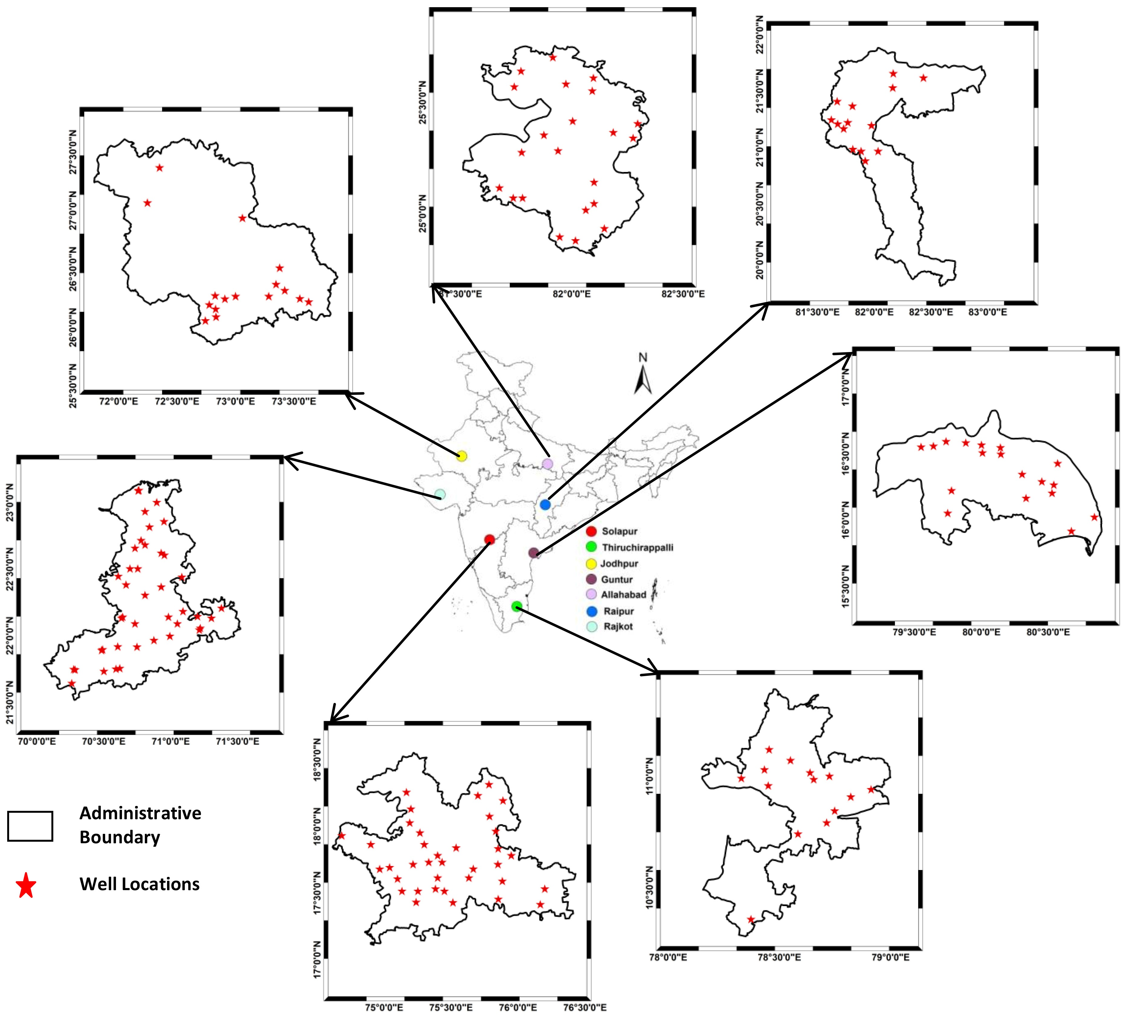
2.1. Study Area and Data Collection

Seven cities (Table 1) were selected based on the following criteria: (i) population ~1 Million (2011 Census) [45], (ii) decadal population growth rate greater than ~15% (2001 to 2011 Census) [45], (iii) high Gross Domestic Product (GDP) and economic growth rate [46], (iv) population density, and (v) shortlisted as a smart city under the urban renewal program, National Smart City Mission, by the government of India [47]. The groundwater level data for the years 1996–2018 has been collected for the selected seven cities from the Central Groundwater Board (CGWB) through the India Water Resource Information system [48]. The CGWB monitors seasonal groundwater levels quarterly (i.e., January—Post-monsoon Rabi, May—Pre-monsoon, August—Monsoon, and November—Post-monsoon) [49]. Grubbs test was used to remove the outliers in the dataset. The Grubbs test statistics are defined as G = m a x Y i     Y ¯ s , where Y i is the ith data point and Y ¯ and s denote the sample mean and standard deviation, respectively. The wells located in the selected cities having at least 18 years of observed data out of a total of 23 years (~80% observations) were selected for the analysis (refer to Figure 1 for the map of the study area and the wells selected for the analyses) [50]. The monthly Terrestrial Water Storage anomalies were obtained from Gravity Recovery and Climate Experiment (GRACE) satellite observations for the months of January, May, August, and November within the study period (2002–2017) to analyze the total water storage in the selected cities [51]. Daily gridded rainfall data (0.25ø × 0.25ø) obtained from the Indian Meteorological Department (IMD) were used to estimate the monthly rainfall values for the selected cities [52]. Moderate Resolution Imaging Spectroradiometer (MODIS) classified LULC maps (MCD12Q1v006: LC_type 4 layer) obtained for the years 2001 and 2018 were used to perform the LULC analysis [53].

2.2. Trend Analysis

The Theil-Sen estimator, a widely used method in detecting trends in a hydrological time series, was employed to determine the nonparametric linear GWL trend (in cm year−1) [38,54], and the significance of the determined trend was estimated by applying the modified Mann–Kendall (MMK) test [39,55]. The Theil-Sen estimator determines the slope between all possible data pairs as, Q i = y j     y k j     k   , where Q i is the slope between data points y j and y k at time j and k , such that j > k and i = 1, 2…n. For n values of the time series of y number of slopes, there is N =   n   n     1 2   values of Q i . The Theil-Sen estimator determines the median slope (Q) as, Q = Q n + 1 2 if N is odd and Q = 1 2 Q N 2 + Q N + 1 2 if N is even [38]. The MMK test uses a modified variance to reduce the influence of autocorrelation on the Mann–Kendall test results [56,57]. The test statistics of MMK are the same as the Mann–Kendall test and are defined as S = i = 1 n 1 j = k + 1 n S i g n x j x k , where S is the test statistics, x j   and x k are the data points observed at time j and k respectively ( j > k ), and n is the length of the dataset [39,56]. The trends in the GWL were estimated in terms of changes in the depth to groundwater table below ground level in centimeters per year. Although several methods exist to recover the GWL from Satellite products (e.g., GRACE [51]), these methods provide only gross estimates with higher uncertainty, bias, and errors [58,59]. To overcome the above issues, GWL observations from monitoring wells by CGWB were used. Though the trend analysis was focused on estimating the temporal trends at the point level (individual wells), the selected wells are uniformly distributed across the city (Figure 1), with each well representing a block (or part) of a city, which subsequently helps to understand the spatial trends as well.

2.3. TWS Anomalies and Groundwater Levels

To understand the extent of changes in the overall water storage (includes surface water, soil moisture, groundwater, etc.), the Terrestrial Water Storage (TWS) anomalies were analyzed. The TWS anomalies data were obtained from the Gravity Recovery Climate Experiment (GRACE) interpolated at 1ø × 1ø grid cells for the selected seven cities for the period 2002 to 2017 [51]. The trends and non-stationarity in the TWS changes were determined, and the results of TWS were correlated with GWL changes in the selected cities.

2.4. Non-Stationarity Analysis

Non-stationarity analyses were performed to assess the impacts of climate change caused by low-frequency climate variability and LULC changes on GWL changes [60]. The most frequently used Augmented Dickey-Fuller (ADF), Phillip-Perron (PP), and Kwiatkowski-Phillips-Schmidt-Shin (KPSS) tests were applied to estimate the non-stationarity in GWL changes [40,41,42].
The ADF test assesses the null hypothesis of a unit root using the model: y t = y t 1 + β 1 Δ y t 1 + β 2 Δ y t 2 + + β p Δ y t p + ε t against the alternative model: y t = ϕ y t 1 + β 1 Δ y t 1 + β 2 Δ y t 2 + + β p Δ y t p + ε t , where y t is the time series with time t, Δ is the differencing operator, β is constant, p is the number of lagged difference terms, and εt is a mean zero innovation process [40,61]. The alternate hypothesis ( ϕ   < 1) in the ADF test is generally stationary or trend stationary [61].
Similar to the ADF test, the PP test assesses the null hypothesis of a unit root in a univariate time series; however, it makes a nonparametric correction to t-statistics, which makes it more robust with unspecified autocorrelation [62,63]. The PP test assesses the null hypothesis using the model:   y t = y t 1 + e t , against the alternative model:   y t = a   y t 1 + e t , where y t is the time series with time t, e t is the innovations process and a is the auto regression coefficient, such that a < 1 [41,63].
The KPSS test, in contrast to ADF and PP tests (which tests for non-stationary as a null hypothesis), assesses the null hypothesis that a univariate time series is trend stationary against the alternate hypothesis of non-stationarity [42]. The KPSS test assesses the null hypothesis of trend stationarity using the models: y t = c t + δ t + u 1 t and c t = c t 1 + u 2 t against the alternate hypothesis of non-stationarity, where c t is the random walk term, δ is the trend coefficient, u1t is a stationary process, and u2t is an independent and identically distributed process with mean 0 and variance σ2 [64]. The null hypothesis σ2 = 0 implies that the random walk term ( c t ) is constant, and the alternative hypothesis σ2 > 0, which introduces the unit root in c t [42,64].
Although the power of non-stationarity tests varies, all the non-stationarity tests are known to have low power (power is determined by auto-regression parameter ϕ1 in case of ADF and PP tests) when the length of the time series is short [65]. However, the KPSS test is an exception and performs well in shorter time series, which made it suitable for our analysis (although the KPSS test has a high rate of Type I Errors (rejection of null hypothesis)) [65,66]. As the availability of the observed GWL data is very limited, the non-stationarity in the GWL changes was confirmed if the majority of the three tests (ADF, PP, and KPSS) suggest non-stationarity. Thus, the bias due to data length was minimized.

2.5. Correlation Analysis: Rainfall and Groundwater Levels

The impacts of climate variability on GWL changes were grossly analyzed by correlating rainfall with GWL changes in the wells having non-stationarity [67]. The relationship between rainfall–groundwater recharge is complex; however, few studies show a high correlation between them [68,69,70]. Since the groundwater system’s recharge characteristics are complex, there is always a time delay between rainfall and the water to reach the groundwater table [68,71]. The cross-correlation was carried out for two conditions such as: (i) no lag and (ii) 3-month lag (or 1 season lag) with the groundwater level data to account for the delay in the recharge of groundwater after the rainfall. For this, the gridded rainfall data and GWL changes from the wells exhibiting non-stationarity behavior and falling within the grid were used. It may be noted that about 94% of the wells used in the analysis are dug wells (lies predominantly in the unconfined aquifers) with depth generally varying between 10 and 30 m, and therefore directly relating the monthly rainfall to GWL changes is justified (not accounting for the recharge from the confined aquifer) [49].

2.6. LULC Change Analysis

The impacts of LULC change on GWL were also quantified. The Moderate Resolution Imaging Spectroradiometer (MODIS) classified LULC maps (MCD12Q1v006: LC_type 4 layer) for the years 2001 and 2018 were used to analyze the LULC changes in the respective cities. This MODIS-MCD12Q1v006 data product for global land cover is available at 500 m resolution [53]. A 15 km radial buffer around the center point of the cities was created since the overlay analysis revealed that the urban expansion between 2001 and 2018 at these selected cities was very much contained within this buffer zone. This 15 km buffer zone shapefile was used to clip out the LULC maps of the respective cities. Google Earth Engine (GEE) algorithms were used to analyze the entire spatial data, starting from accessing the data to the creation of the LULC change map. The impact of change in LULC components on GWLs was assessed through performing correlation analysis between the percentage of wells having significant increasing/decreasing GWL trends (>2 cm/year) and LULC change between 2001 and 2018 at the city level. The statistical analyses were also performed for the wells located outside the urban boundary as these cities have high scope for expansion in terms of infrastructural growth and socio-economic activities.

3. Results and Discussion

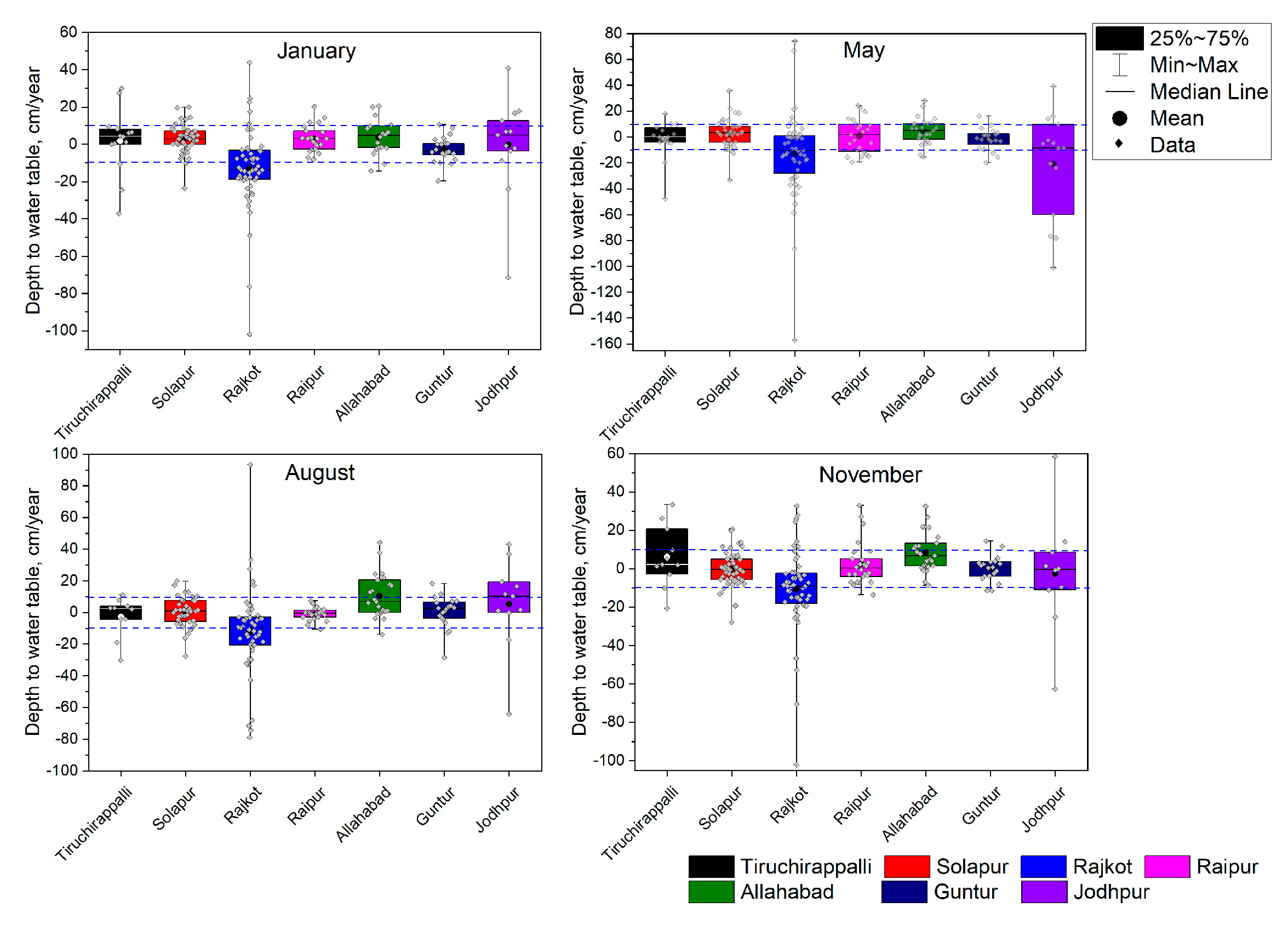
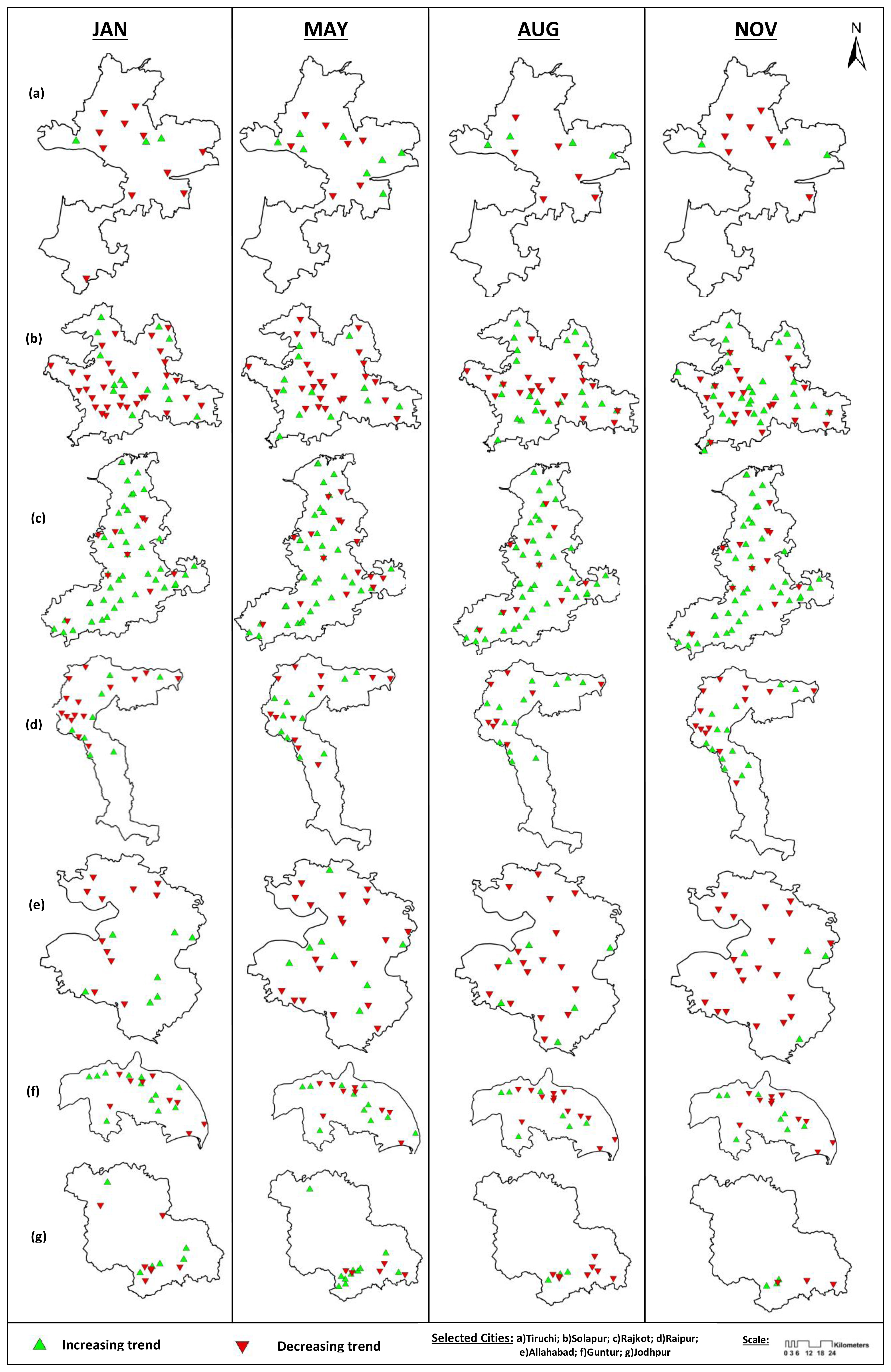
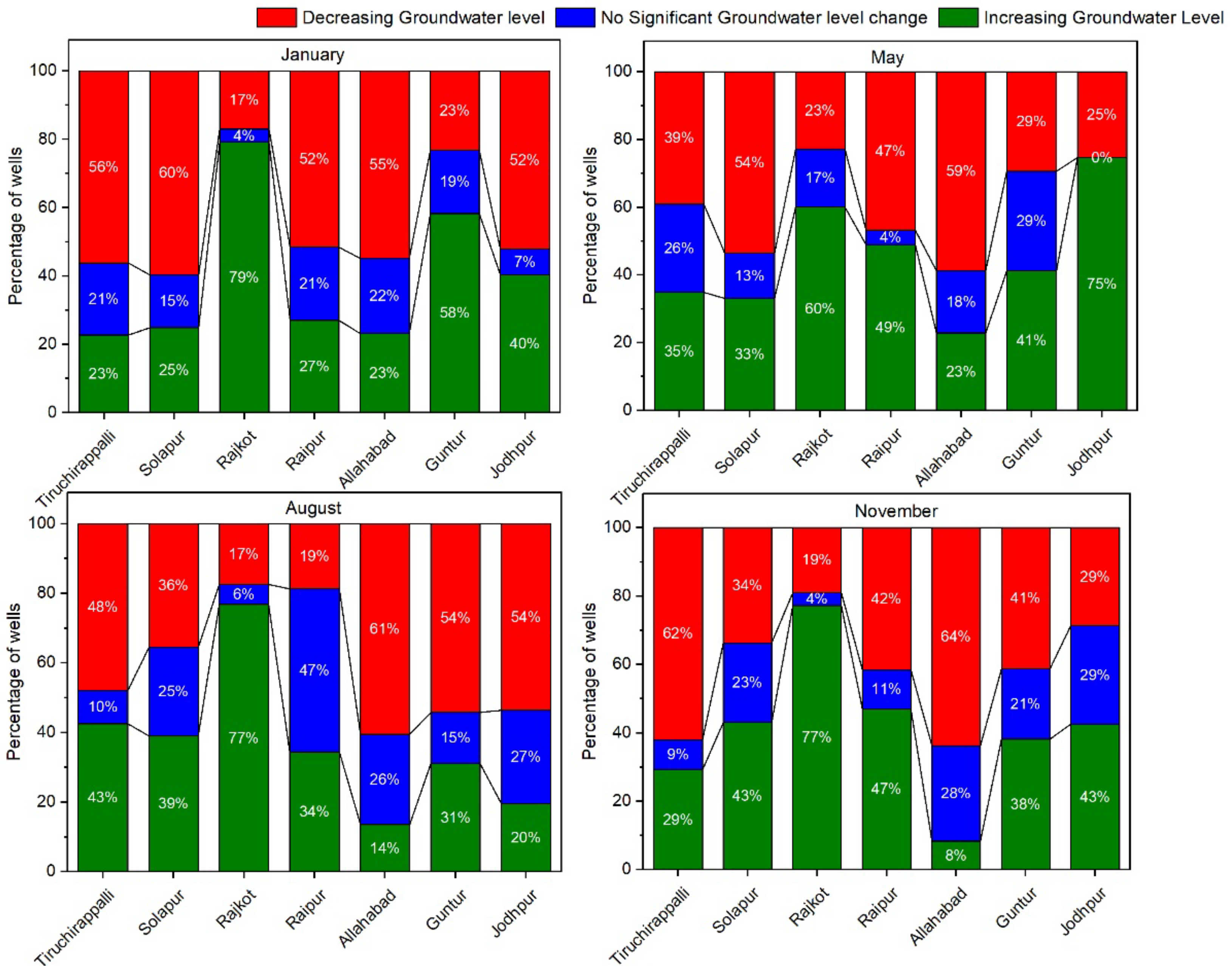
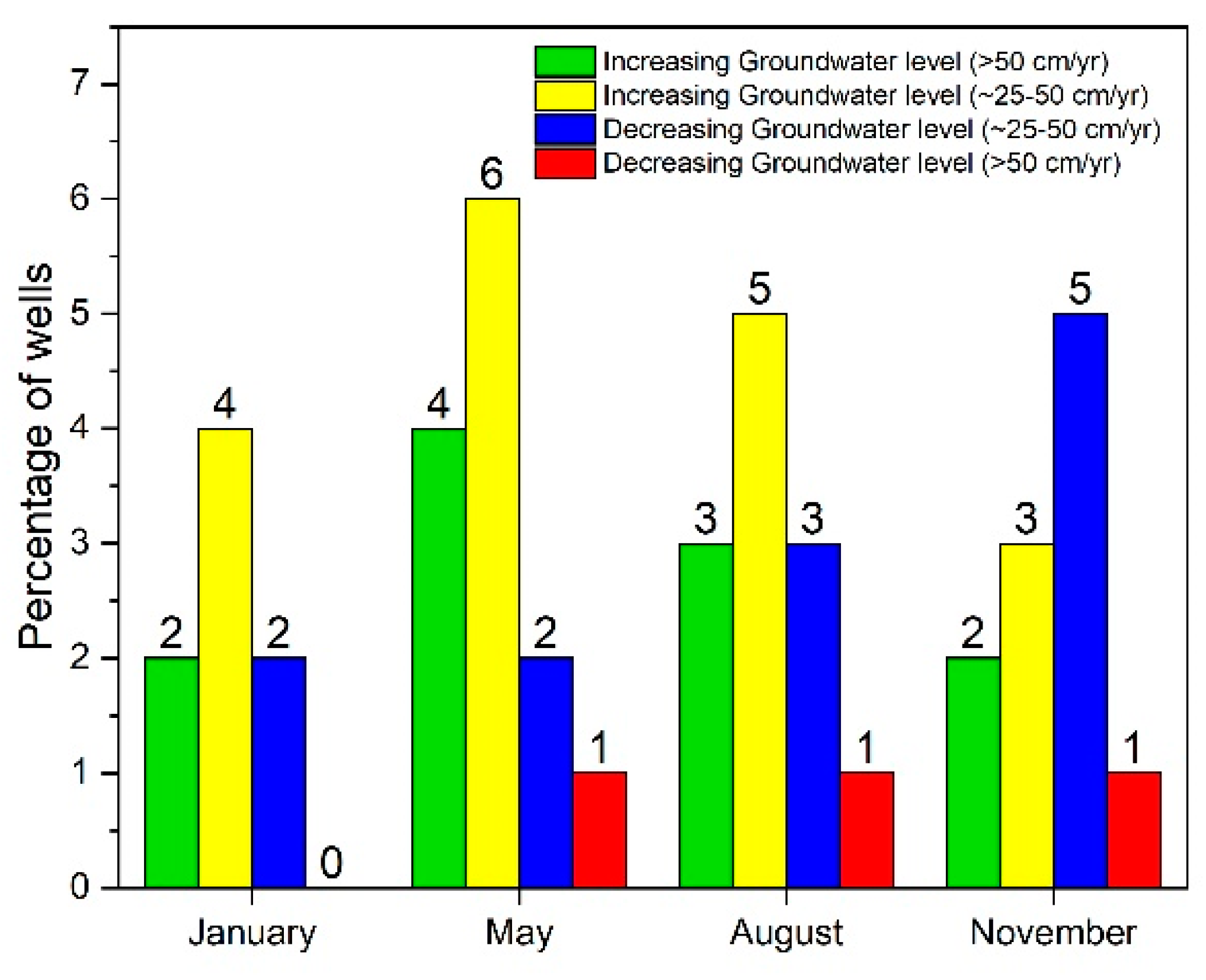
3.1. Trends in Groundwater Level Changes

Trend analysis for GWL changes revealed that the GWL majorly varied between ±~10 cm/year (Figure 2) across the selected cities. Spatially, GWL trends (Figure 3) were found to be decreasing in the majority of the wells, except in Rajkot and Guntur. In general, consistent high decreasing and low increasing GWL trend patterns were observed in January relatively, compared to other months of observation (Figure 2). A high increasing GWL trend was found in May (Figure 2, Figure 3 and Figure 4), though May is considered to have peak summer with high evapotranspiration losses and very few rain spells in India [72,73]. This anomaly, however, can be attributed to changes in the characteristics and spatial-temporal variability of rainfall events in India [74,75]. Very similar GWL trends across the seasonal data collected in January, May, August, and November (Figure 2) were observed, which suggests a less interdependence between seasonality and GWL trends. However, the lower tail of the box plot (Figure 2) indicates a sharp increase in GWL, and this behavior could be attributed to groundwater recharge from the monsoon rainfall [15,16]. Similarly, the upper tail of the box plot indicates a sharp decline in GWL that might be due to excessive pumping [16]. Overall, a higher magnitude GWL trend (increasing as well as decreasing) greater than ~25–100 cm/year throughout the seasons from January to November was observed, which might be due to the effect of climate variability and/or anthropogenic activities [76,77,78].
Figure 2 also illustrates the magnitude of GWL variability among the selected cities. A higher magnitude of decreasing GWL trends was noticed in Allahabad (especially in August and November), followed by Jodhpur. However, in Jodhpur, a high-magnitude increasing trend was also found in some proportion of the wells throughout the seasons (January to November). A high magnitude of increasing GWL trend was detected in Rajkot, which confirms a very high rate of increasing GWL in the western arid regions of India, as reported in previous studies [16,79]. A similar magnitude of increasing and decreasing GWL was observed in Guntur from January to November. However, in May, a relatively higher decreasing GWL trend in Guntur was found, with more than 20% of wells declining at a rate greater than 10 cm/year. This might be due to a high surge in pumping during the peak of a seasonal dry spell since Guntur’s economy is highly dependent on agricultural and allied activities [80]. Tiruchirappalli and Solapur exhibited similar behavior in terms of resulting slightly higher magnitude of declining GWL. Except for Rajkot, where the GWL was increasing in the majority of wells between ~2 to 20 cm/year, the overall groundwater level was found to be increasing or decreasing at ~10 cm/year in all other selected cities.
There were no significant GWL changes (Figure 4) in about ~7–29% (with exception to Rajkot during January (4%), August (6%), and November (4%), and Raipur in May (4%) and August (47%)) of the wells throughout the study period (we assumed that there is no significant GWL trend if the GWL is varying at ±2 cm/year) in all these selected cities. In the selected cities, increasing and decreasing GWL trend was found in ~8–79% and ~17–64% of wells respectively, from January to November. The city-level results suggested that Rajkot has the highest (60–79%) percentage of wells with a significant increasing GWL trend (greater than 2 cm/year). In contrast, Allahabad has the highest percentage of wells (55–64%) with a significant decreasing GWL trend (greater than 2 cm/year). Raipur was determined to have an almost equal percentage of wells with significant increasing and decreasing GWL in May and November. Overall, the percentage of wells with a decreasing trend was found to be higher than the increasing trend. This reveals groundwater depletion is evident in most of the developing cities across India, which may threaten urban water security [8].
Further, analyses were conducted to find the percentage of wells having extreme increasing or decreasing GWL trends (Figure 5). Since the Theil-Sen slope estimates the median trend from a combination of slopes, it is important to note that the magnitude of the actual trend (increasing or decreasing) might be much higher than the trend estimated using the Theil-Sen slope method. Based on the thresholds of ~25 and ~50 cm/year, the percentage of wells having an extreme GWL trend during the study period was determined. In the first half of the year (i.e., January and May), the percentage of wells with increasing GWL was found to be higher than that of decreasing GWLs in the selected cities. However, at the end (November), opposite behavior was observed for which the percentage of wells having a decreasing GWL was high. This might be due to the excessive rate of pumping in November, mainly to manage the water shortage caused by the lack of rainfall during the post-monsoon season across India [74].

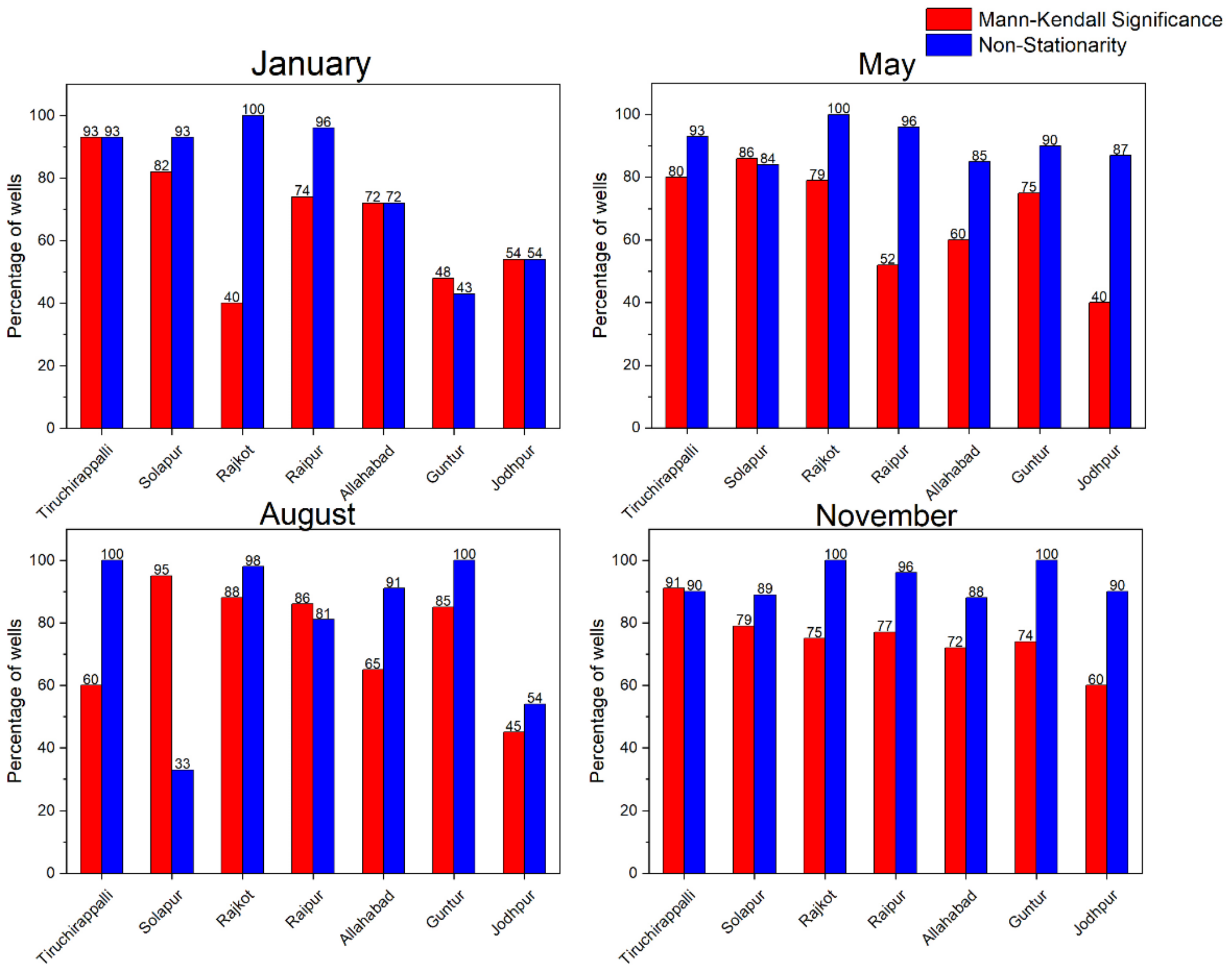
3.2. Non-Stationarity and Significance of Groundwater Level Trends

The significance of GWL trends was estimated using the MMK test. Based on the results (Figure 6), we found that ~40–93% of the wells in the selected cities had a significant trend during the different months of study (i.e., a monotonic trend is present, and the trend is statistically significant), with the highest MMK significance observed consistently in November (60–91% of wells showed a significant trend). Similarly, the significance of the trend at the city level was found to be in higher proportions in Solapur (79–95% of wells), followed by Tiruchirappalli (80–93% of wells, except in August). The significance of trend was found to be relatively minimal in Jodhpur and Guntur.
The combined results (Figure 6) of ADFT, KPSS, and PP tests showed that ~70–100% of the wells exhibited non-stationarity across different months (i.e., January to November). Notably, in November, about 90–100% of the wells (Figure 6) exhibited non-stationarity. At the city level, non-stationarity was observed in almost all the wells in Rajkot (98–100%) from January to November. On the other side, non-stationarity is least in Solapur, with 33% of wells (observed in August), followed by Jodhpur, which has non-stationarity in only 54% of wells during May and August. It can be understood from these results that the majority of the wells in these cities (at least more than 50%) may be significantly affected by climate variability and LULC change. The presence of such high non-stationarity would create huge uncertainty in the behavior of groundwater systems, which makes it difficult to predict future GWLs. Subsequently, this might lead to complex problems in different spheres, especially in development, public health, and irrigation, in the selected rapidly growing secondary cities [81].
About ~27–33% of wells in the selected cities were determined to have a decreasing GWL trend along with MMK trend significance and non-stationarity in GWL changes. At the city level, this behavior was found to be highest in Tiruchirappalli (64% of wells) and least in Rajkot (12% of wells). Notably, Jodhpur, the city with high decreasing GWL, has only ~20% of wells with this behavior. Interestingly, we determined that there was no non-stationarity as well as the MMK trend significance in wells present in the regions of high decreasing GWL trend, i.e., Rajkot and Allahabad. Although these cities (i.e., Rajkot and Allahabad) have high increasing and decreasing GWL (Figure 4 and Figure 5, respectively), the percentage of wells having non-stationarity and MMK trend significance were relatively lower among the selected cities.

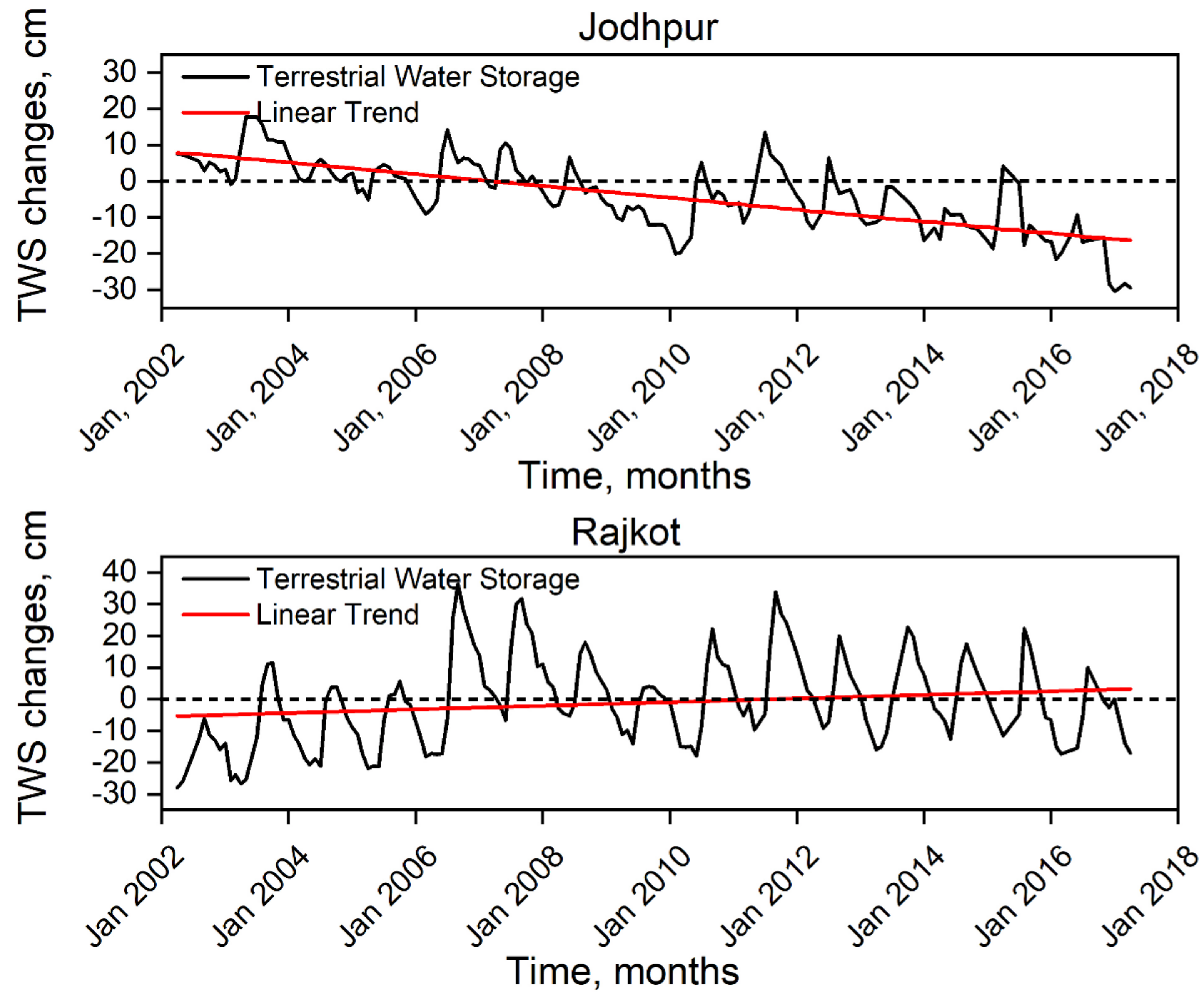
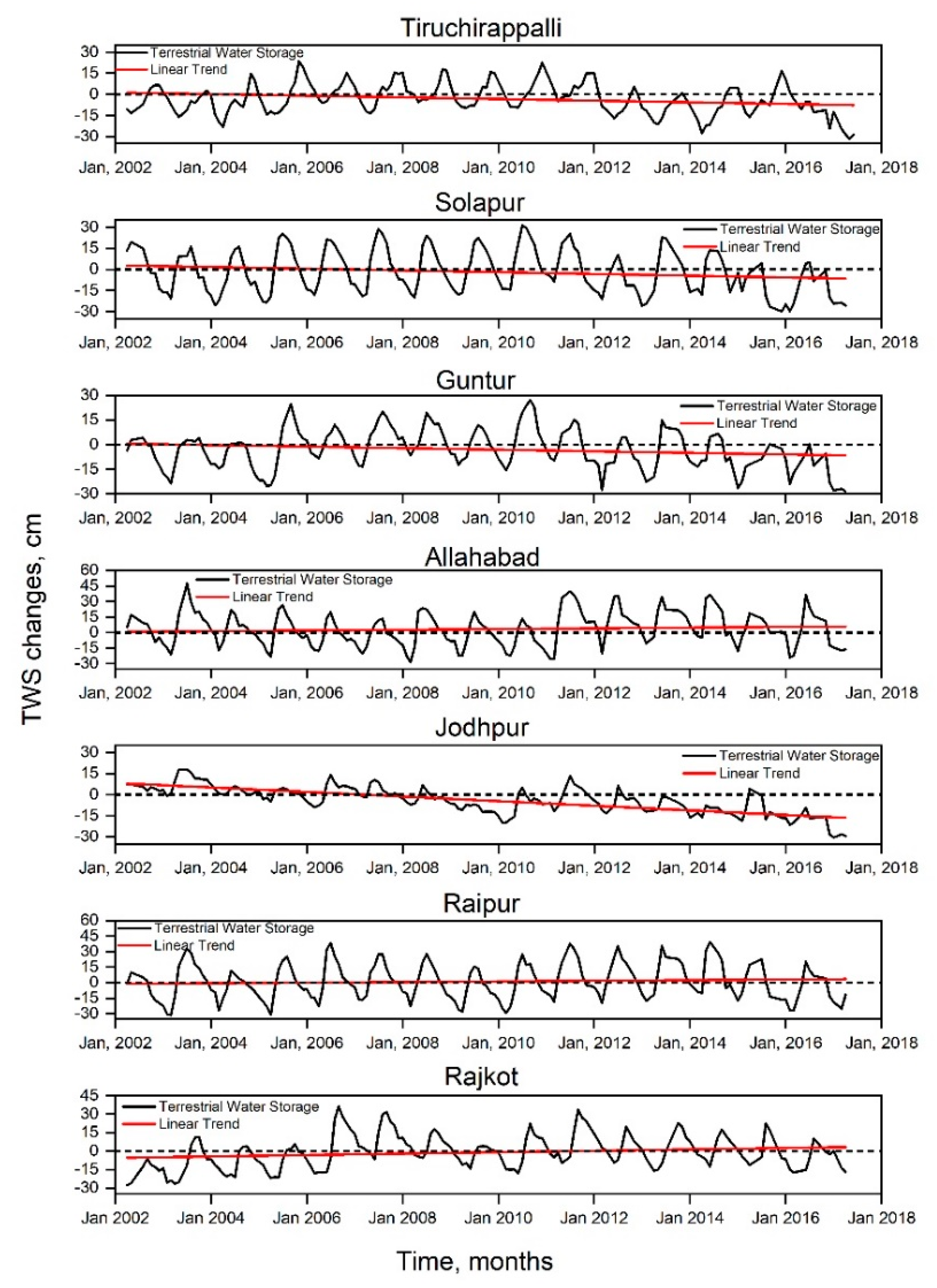
3.3. Terrestrial Water Storage Anomalies

The Theil-Sen trend in TWS anomalies (Figure 7) was estimated, and the highest declining TWS trend was observed in Jodhpur (−1.79 cm/year) (Table 2). On the contrary, TWS is highly increasing in Rajkot at 0.67 cm/year among the selected cities. While high non-stationarity was found in the GWL changes, non-stationarity in TWS anomalies was not observed in any of the selected cities. Similarly, MMK trend significance was also found to be absent in cities with a higher magnitude of increasing or decreasing TWS trends (Rajkot and Jodhpur). Unlike the GWL changes, the TWS trends indicate that the overall water storage or the TWS cycle (including surface water, soil moisture, etc., including groundwater) in the selected secondary cities have not majorly been affected by climate variability and LULC changes [51]. However, comparing the changes in TWS anomalies with GWL, a high positive correlation was observed both in the case of increasing (R = 0.85) and decreasing (R = 0.87) trends. Refer to Appendix A Figure A1 for TWS trends of all the selected cities.

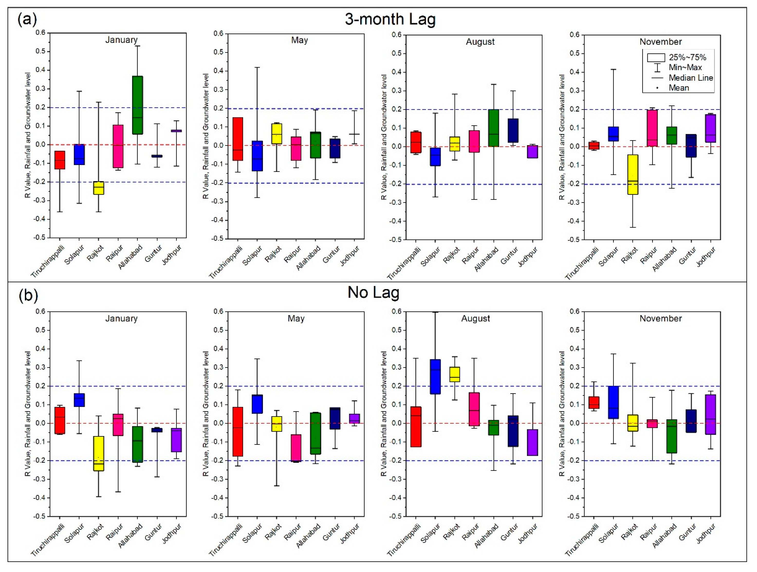
3.4. Rainfall and Groundwater Level Change Relationship

The response of GWL to rainfall was investigated through correlation analysis for the period 1996–2018. The correlation analysis on the wells having non-stationarity in the selected cities revealed that there is no strong dependency between rainfall and GWL changes. Figure 8 shows the box plot of the Correlation Coefficient (R) values for all the wells with non-stationarity. The positive R-value indicates that the GWL increases with rainfall and vice versa. The R-value varying between ±0.2 was found in ~95% of the wells for both no lag and three months lag (with the exception of Allahabad in January (under 3-month lag scenario) and Solapur and Rajkot in August (under no lag scenario)), as illustrated in Figure 8. In the 3-month lag scenario (Figure 8a), negative R values were observed in the majority of the wells, notably in Rajkot (both in January and November). A similar observation was noted for the no lag scenario (Figure 8b); however, the tail ends were shorter in the box plot in August and November. Since the majority of the wells (dug wells with depth ~10–30m) considered in this paper are shallow wells, the recharge time delay is comparatively small. Therefore, no lag scenario might be considered as a realistic scenario [71]. Although from the results of correlation analysis, no good rainfall–GWL response relationship could be drawn-out in the selected cities for January, May, and November, the R values were relatively high in Solapur, Rajkot, and Raipur in the month of August in the no lag scenario. While there is comparatively a good correlation between rainfall and GWL observed in August in the above cities, the percentage of wells with significant declining GWL trends was observed only in 20–36% of wells (Figure 4). In contrast to August, poor rainfall–GWL response was observed in January in which almost all the wells in Rajkot, Guntur, and Allahabad showed a negative correlation. January, which has a poor R-value in the no lag scenario (Figure 7b), has a relatively higher proportion of wells with decreasing GWL in Allahabad, Jodhpur, and Solapur (Figure 3 and Figure 4), which suggests that declining GWL have a strong correlation with decreasing recharge from rainfall. The correlation analysis suggests that the rainfall and groundwater recharge relationship has been seriously affected and also ascertains the lack of seasonality in the GWL trends in the selected cities. This confirms the high variability in the rainfall events and the delay (and sometimes even failure) in the monsoon rainfall, as reported in previous studies across India [74,75,82]. The results also strongly suggest that climate variability (rainfall) has affected the GWL trends in the selected cities.

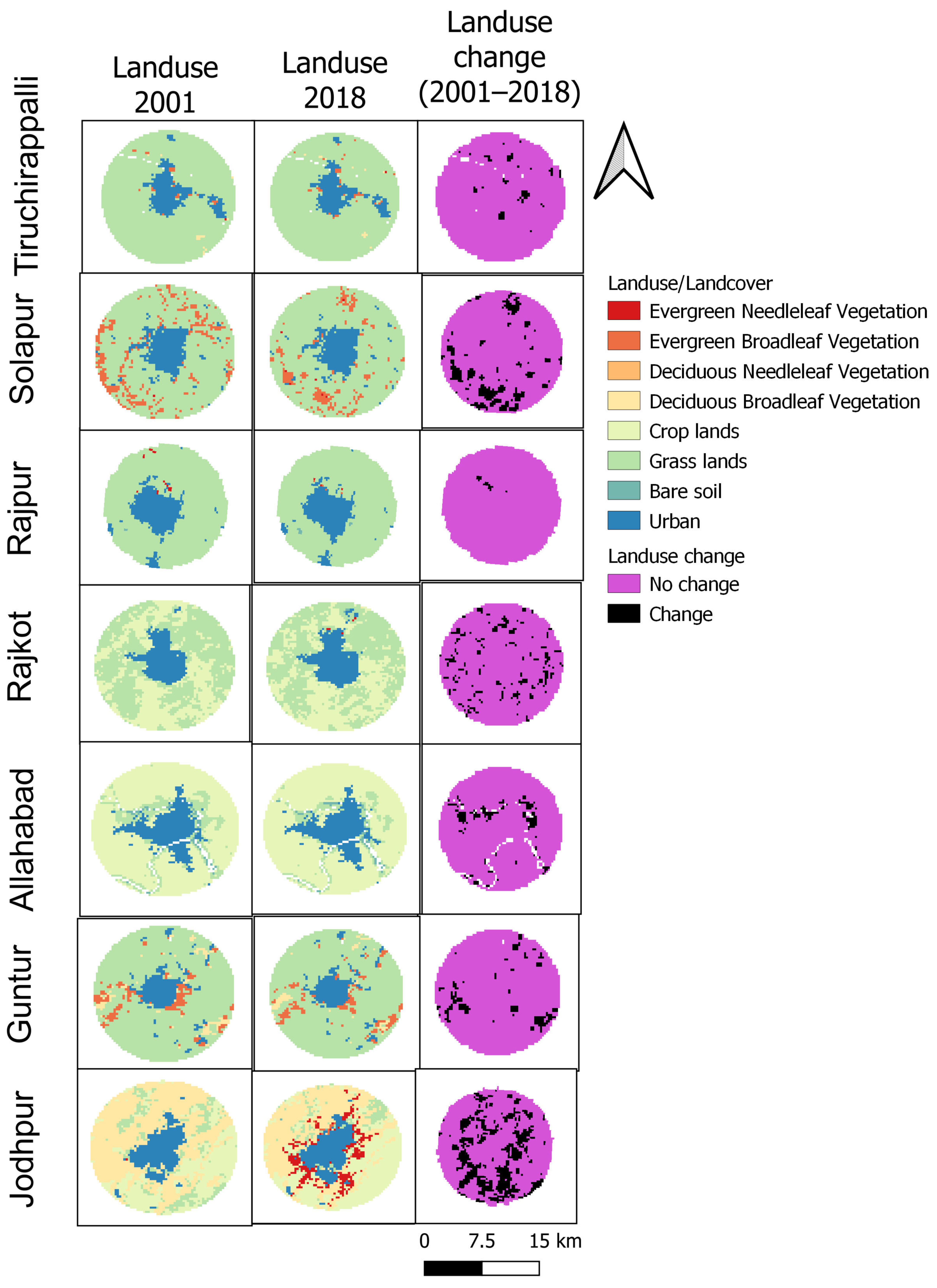
3.5. Impact of Land Use/Land Cover Changes on Groundwater Level

LULC analysis (Figure 9) was performed using MODIS images collected between the years 2001 and 2018 (refer to Table 3 for detailed LULC area changes in the selected cities). Overall, the conversion of vegetation into grassland and croplands was majorly observed in all the selected cities. A relatively high growth in the urban area was seen in Raipur and Rajkot (1.6% and 2% increase, respectively), followed by Jodhpur (1.4% increase). However, in other cities, the urban area growth was less than ~0.5%, with almost no growth in the urban area of Tiruchirappalli. The higher rate of population growth (12–45% based on the census), burgeoning real-estate activities, mainly to convert agricultural fields and uncultivated land into barren land (plots) for domestic housing and industrial expansion, clearing land for road construction and highways projects, increasing the urban built area, etc. [83,84], could be considered as the main factors for the LULC changes during the study period. Notably, the high growth of the urban area in Raipur might be attributed to the city being declared as the capital of the state Chhattisgarh after its partition from Madhya Pradesh in 2001 [85]. Exponential industrial and infrastructural growth in Raipur in the past two decades has led the city to transform into a major economic hub in the region [85,86,87]. The LULC change trends observed in Raipur during the study could be expected in other secondary developing cities in the future, where rapid migration, infrastructural and industrial growth, etc., could lead to major LULC changes (especially the conversion of the green cover into barren land) and the sudden change might create acute stress on groundwater systems [22,87]. Unlike the metropolitans, where the growth of the urban area is very high in the outskirts of the city, the seven cities in this study show no significant expansion of urban areas outside the pre-existing urban boundary. This implies that major economic activities in the secondary Indian cities primarily take place within the existing urban boundaries, as reported in previous studies [88,89]. This subsequently indicates that most of the infrastructural developments are progressing without significantly reducing green cover in these selected cities. Within the seven cities, the highest LULC changes (Figure 9) were observed in Jodhpur, followed by Solapur and Rajkot. In Jodhpur, the cropping practice has changed, and the cropping area has increased significantly (increased by 8%) during the study period, which might be the reason for the high decreasing GWL in the region due to increased water requirement for irrigation activities [90].
On the other hand, in Rajkot, although a significant decline in the Grasslands area (green cover) occurred, the GWL trends in Rajkot are better than other cities. This trend, however, is recently observed mainly in the western arid states, which might be due to improved rainfall–GWL relationships. The positive (R = 0.14) and negative (R = −0.22) correlation coefficients were observed when cross-correlating decreasing and increasing GWL respectively, with the increase in urban areas. This strongly suggests that GWL decreases with an increase in the urban area (Table 4). These results are also in good agreement with other recent studies and suggest that LULC has a significant impact on GWL in developing cities [36,91]. Also, a very high correlation between the increase in the bare soil (decreasing green cover) area and decreasing GWL (R = 0.93) was observed. Thus, the major influence on decreasing GWL could be attributed to the conversion of the green cover into barren land for various anthropogenic activities such as infrastructural development, real-estate, etc. It may be inferred from these results that the irrigation and agricultural water requirements, although expected to have a very high impact on decreasing GWL in the selected developing cites (since most of the selected cities are still having major agricultural activities outside the urban boundary), are not the major driver; however, the conversion of the green cover (majorly the cropping area) into barren land has more influence on decreasing GWL. LULC change analyses also reveal that an increase in the urban area has a significant impact on decreasing GWL. However, the extent of the impact is comparatively lower (R = 0.14), which could be due to the proper functioning of the public water supply schemes and lower domestic water demands. However, as the urban area increases in the future, the stress on GWL might also increase in the selected cities, as previously observed in other already developed Indian cities [92,93].

4. Conclusions

This paper focused on understanding the GWL trends in the secondary developing cities in India. Seven cities were selected for the analysis based on various aspects, including the socio-economic and population growth trajectories. The key findings were derived based on statistical and LULC change analysis performed on the GWL data. Overall, it was found that the GWL varies between ±10 cm/year, with the trend to be significant (MMK test) in the majority of the wells. Non-stationarity was observed in the majority of the wells throughout the seasons, which suggests GWL has been affected by both climate variability (in monsoon rainfall) and LULC change. However, wells having a high decreasing GWL trend mostly did not exhibit non-stationarity in GWL changes. This indicates that the declining GWL of higher magnitudes has no substantial variation, possibly due to irreversible aquifer depletion caused by a high rate of pumping over a long time, where the effects of climate variability and LULC changes might be negligible. Less interdependence between seasonality (based on monsoon) and GWL trends was observed, which might have been caused by the impact of climate variability on groundwater recharge. The cause of non-stationarity in GWL was analyzed by linking climate variability (rainfall) and LULC with the GWL changes. Correlation analysis between GWL and rainfall indicates that the rainfall–groundwater level relationship has been seriously affected across all the selected cities, plausibly due to the failure of monsoon rainfall. Based on LULC change analysis, a high correlation between decreasing green cover (increasing barren land) (R = 0.93) and decreasing GWL indicates a high anthropogenic activity. Although agriculture-based activities are still actively practiced in secondary developing cities, its impact on GWL was surprisingly relatively low. The change in the urban area was majorly within the pre-existing urban boundary, and the domestic water requirement presently might not contribute much to the decreasing GWL. However, with more urbanization, this might change in the future. The major findings of this study can very well be adopted in other secondary developing cities with similar socio-economic growth patterns, especially in developing countries.
Instead of using the derived GWLs from satellite products, which are considered to contain more error and uncertainty, this paper used point scale well observations to assess the trends and non-stationarity in GWL changes. However, the bias in the trend and non-stationarity estimates are still possible due to the limitations in the data length and the number of available observation wells. Therefore, future research works, including the more observed data to conduct a similar study, are recommended.

Author Contributions

Conceptualization, K.S.K. and B.-S.S.; methodology, K.S.K., J.H. and S.M.; software, K.S.K., S.M., M.M.D.M. and A.M.; validation, I.I. and K.S.K.; formal analysis, K.S.K. and S.M.; investigation, K.S.K., J.H., S.M.P., B.-S.S., S.M. and I.I.; data curation, A.M.; Writing, K.S.K., I.I. and B.-S.S.; Review, K.S.K., J.H., S.M.P., B.-S.S., M.M.D.M. and I.I.; visualization, K.S.K. and I.I.; supervision, K.S.K. All authors have read and agreed to the published version of the manuscript.

Funding

This research received no external funding.

Acknowledgments

The authors wish to thank the Editor and four anonymous reviewers for their constructive comments and suggestions, which helped to improve the complete structure of the paper. This research work was supported by the Early Career Research Award from SERB, Government of India (File NO.ECR/2018/002136), received by the corresponding author.

Conflicts of Interest

The authors declare no conflict of interest.

Appendix A

Figure A1. Terrestrial Water Storage (TWS) changes w.r.t time in the selected cities.
Water 12 03209 g0a1

References

  1. Margat, J.; Gun, J. Groundwater around the World, 1st ed.; CRC Press: London, UK, 2013. [Google Scholar] [CrossRef]
  2. Mullen, K. Groundwater Information on Earth’s Water. Available online: https://www.ngwa.org/what-is-groundwater/About-groundwater/information-on-earths-water (accessed on 26 October 2020).
  3. Zektser, I.S.; Everett, L.G. Groundwater Resources of the World and Their Use. UNESCO Digital Library. Available online: https://unesdoc.unesco.org/ark:/48223/pf0000134433 (accessed on 14 June 2020).
  4. Siebert, S.; Burke, J.; Faures, J.; Frenken, K.; Hoogeveen, J.; Döll, P.; Portmann, F. Groundwater use for irrigation—A global inventory. Hydrol. Earth Syst. Sci. 2010, 14, 1863–1880. [Google Scholar] [CrossRef] [Green Version]
  5. Vörösmarty, C.; McIntyre, P.; Gessner, M.; Dudgeon, D.; Prusevich, A.; Green, P. Global threats to human water security and river biodiversity. Nature 2010, 467, 555–561. [Google Scholar] [CrossRef]
  6. 68% of the World Population Projected to Live in Urban Areas by 2050, Says U.N. Available online: https://www.un.org/development/desa/en/news/population/2018-revision-of-world-urbanization-prospects.html (accessed on 26 October 2020).
  7. Elfie, S.; Denise, P.; Eric, D. The future of India’s urbanization. Futures 2014, 56, 43–52. [Google Scholar] [CrossRef] [Green Version]
  8. Foster, S.; Hirata, R. Groundwater use for urban development: Enhancing benefits and reducing risks. Water Front. 2011, 2011, 21–29. [Google Scholar]
  9. Howard, K.; Hirata, R.; Warner, K.; Gogu, R.; Nkhuwa, D. Resilient Cities & Groundwater. In IAH Strategic Overview Series; Stephen, F., Gillian, T., Eds.; International Association of Hydrogeologists: London, UK, 2015; Available online: https://www.iges.or.jp/en/pub/resilient-cities-groundwater/en (accessed on 26 October 2020).
  10. The United Nations World Water Development Report 2015: Water for a Sustainable World. Available online: https://unesdoc.unesco.org/ark:/48223/pf0000231823 (accessed on 13 November 2020).
  11. Donald, R.I.; Katherine, W.; Julie, P.; Martina, F.; Christof, S. Water on an urban planet: Urbanization and the reach of urban water infrastructure. Glob. Environ. Chang. 2014, 27, 96–105. [Google Scholar] [CrossRef] [Green Version]
  12. Bricker, S.H.; Banks, V.J.; Galik, G. Accounting for groundwater in future city visions. Land Use Policy 2017, 69, 618–630. [Google Scholar] [CrossRef]
  13. Foster, S.D.; Ricardo, H.; Ken, W.F.H. Groundwater use in developing cities: Policy issues arising from current trends. Hydrogeol. J. 2010, 19, 271–274. [Google Scholar] [CrossRef]
  14. Tiwari, V.; Wahr, J.; Swenson, S. Dwindling groundwater resources in northern India, from satellite gravity observations. Geophys. Res. Lett. 2009, 36. [Google Scholar] [CrossRef] [Green Version]
  15. Chatterjee, R.; Purohit, R. Estimation of Replenishable Groundwater Resources of India and Their Status of Utilization. Curr. Sci. 2009, 96, 1581–1591. [Google Scholar]
  16. Asoka, A.; Gleeson, T.; Wada, Y.; Mishra, V. Relative contribution of monsoon precipitation and pumping to changes in groundwater storage in India. Nat. Geosci. 2017, 10, 109–117. [Google Scholar] [CrossRef] [Green Version]
  17. Rodell, M.; Velicogna, I.; Famiglietti, J. Satellite-based estimates of groundwater depletion in India. Nature 2009, 460, 999–1002. [Google Scholar] [CrossRef] [Green Version]
  18. Hora, T.; Srinivasan, V.; Basu, N. The Groundwater Recovery Paradox in South India. Geophys. Res. Lett. 2019, 46, 9602–9611. [Google Scholar] [CrossRef]
  19. Gana, K. Uncovering the Groundwater Crisis in South India. Available online: https://india.mongabay.com/2019/09/uncovering-the-groundwater-crisis-in-south-india (accessed on 26 October 2020).
  20. Singh, R.B. Impact of land-use change on groundwater in the Punjab-Haryana plains, India. In Proceedings of the Impact of Human Activity on Groundwater Dynamics, Maastricht, The Netharlands, 18 July 2001; IAHS-AISH Publication: Wallingford, UK, 2001; pp. 117–122. [Google Scholar]
  21. Samanpreet, B.; Rajan, A.; Mandeep, B. Groundwater Depletion in Punjab, India. In Encyclopedia of Soil Science, 3rd ed.; Tylor & Francis: Abingdon-on-Thames, UK, 2017; pp. 1–5. [Google Scholar] [CrossRef]
  22. Foster, S. Global Policy Overview of Groundwater in Urban Development—A Tale of 10 Cities. Water 2020, 12, 456. [Google Scholar] [CrossRef] [Green Version]
  23. Ken, W.H.F. Urban Groundwater: Meeting the Challenge; IAH Selected Paper Series 8; CRC Press: Boca Raton, FL, USA, 2007; ISBN 9780415407458. [Google Scholar]
  24. NITI. Aayog Composite Water Management Index 2.0. Available online: https://niti.gov.in/sites/default/files/2019-08/CWMI-2.0-latest.pdf (accessed on 26 October 2020).
  25. Chennai Water Crisis: City’s Reservoirs Run Dry. Available online: https://www.bbc.com/news/world-asia-india-48672330 (accessed on 26 October 2020).
  26. Service Level Benchmarks. Available online: http://mohua.gov.in/cms/Service-Level-Benchmarks.php (accessed on 26 October 2020).
  27. Gontoju, S.S.; Alam, M.F.; Sikka, A. Chennai Water Crisis: A Wake-Up Call for Indian Cities. Available online: https://www.downtoearth.org.in/blog/water/chennai-water-crisis-a-wake-up-call-for-indian-cities-66024 (accessed on 18 October 2020).
  28. Aspinwall, N. Chennai’s ‘Man-Made’ Water Crisis. Available online: https://thediplomat.com/2019/08/chennais-man-made-water-crisis (accessed on 25 October 2020).
  29. World Water Day: India is 3rd Largest Groundwater Exporter, but 21 Cities are Running out of Water by 2020. Available online: https://www.indiatoday.in/science/story/world-water-day-2019-water-crisis-india-1483777-2019-03-22 (accessed on 26 October 2020).
  30. Singh, S.; Sharma, V. Urban Droughts in India: Case Study of Delhi. Disaster Risk Reduct. 2018, 155–167. [Google Scholar] [CrossRef]
  31. Sinan, M.; Mishra, V. Urban Drought in India under Observed and Projected Future Climate. In Proceedings of the AGU Fall Meeting, Washington, DC, USA, 10–14 December 2018. [Google Scholar]
  32. Alipour, A.; Hashemi, S.; Shokri, S.; Moravej, M. Spatio-temporal analysis of groundwater level in an arid area. Int. J. Water 2018, 12, 66. [Google Scholar] [CrossRef]
  33. Jessica, H.; Katherine, C.; George, K. Tools to Estimate Groundwater Levels in the Presence of Changes of Precipitation and Pumping. J. Water Resour. Prot. 2016, 8, 12. [Google Scholar] [CrossRef] [Green Version]
  34. Gurdak, J.J.; Kuss, A.M. Teleconnections in the Principal Aquifers to Non-Stationarity of ENSO, NAO, PDO, and AMO. In Proceedings of the AGU Fall Meeting, Washington, DC, USA, 10–14 December 2012. [Google Scholar]
  35. Graf, R. Reference statistics for the structure of measurement series of groundwater levels (Wielkopolska Lowland, western Poland). Hydrol. Sci. J. 2015, 60, 1587–1606. [Google Scholar] [CrossRef]
  36. Kayet, N.; Chakrabarty, A.; Pathak, K.; Sahoo, S.; Mandal, S.; Fatema, S. Spatiotemporal LULC change impacts on groundwater table in Jhargram, West Bengal, India. Sustain. Water Resour. Manag. 2018, 5, 1189–1200. [Google Scholar] [CrossRef]
  37. Roy, A.; Inamdar, A. Multi-temporal Land Use Land Cover (LULC) change analysis of a dry semi-arid river basin in western India following a robust multi-sensor satellite image calibration strategy. Heliyon 2019, 5, e01478. [Google Scholar] [CrossRef] [Green Version]
  38. Pranab, K.S. Estimates of the Regression Coefficient Based on Kendall’s Tau. J. Am. Stat. Assoc. 1968, 63, 1379–1389. [Google Scholar] [CrossRef]
  39. Hamed, K.; Rao, A.R. A modified Mann-Kendall trend test for autocorrelated data. J. Hydrol. 1998, 204, 182–196. [Google Scholar] [CrossRef]
  40. Dickey, D.A.; Fuller, W.A. Distribution of the estimation of autoregressive time series with a unit root. J. Am. Stat. Assoc. 1979, 74, 427–431. [Google Scholar]
  41. Phillips, P. Testing for a unit root in time series regression. Biometrika 1988, 75, 335–346. [Google Scholar] [CrossRef]
  42. Kwiatkowski, D.; Phillips, P.C.B.; Schmidt, P.; Shin, Y. Testing the null hypothesis of stationarity against the alternative of a unit root. J. Econom. 1992, 54, 159–178. [Google Scholar] [CrossRef]
  43. Fathian, F.; Saeed, M.; Ercan, K. Identification of trends in hydrological and climatic variables in Urmia Lake Basin, Iran. Theor. Appl. Climatol. 2014, 119, 443–464. [Google Scholar] [CrossRef]
  44. Navas, R.; Alonso, J.; Gorgoglione, A.; Vervoort, R.W. Identifying climate and human impact trends in streamflow: A case study in Uruguay. Water 2019, 11, 1433. [Google Scholar] [CrossRef] [Green Version]
  45. Census of India. Available online: https://censusindia.gov.in (accessed on 26 October 2020).
  46. Mapping India’s GDP. Available online: https://www.idfcinstitute.org/projects/transitions/city-gdp/ (accessed on 20 October 2020).
  47. Smart Cities Mission. Available online: http://smartcities.gov.in/content/ (accessed on 26 October 2020).
  48. Water Resource Information System, India-WRIS. Available online: https://indiawris.gov.in/wris/#/groundWater (accessed on 26 October 2020).
  49. Central Ground Water Board. Available online: http://cgwb.gov.in/ (accessed on 26 October 2020).
  50. Grubbs, F.E. Procedures for Detecting Outlying Observations in Samples. Technimetrics 1916, 11, 1–21. [Google Scholar] [CrossRef]
  51. Monthly Mass Grids GRACE Tellus Data. Available online: https://grace.jpl.nasa.gov/data/get-data/monthly-mass-grids-land (accessed on 25 October 2020).
  52. Pai, D.S.; Latha, S.; Rajeevan, M. Development of a new high spatial resolution (0.25° × 0.25°) Long period (1901–2010) daily gridded rainfall data set over India and its comparison with existing data sets over the region. Mausam 2014, 65, 1–18. [Google Scholar]
  53. Friedl, M.; Sulla-Menashe, D. MCD12Q1 MODIS/Terra+Aqua Land Cover Type Yearly L3 Global 500m SIN Grid V006; NASA EOSDIS Land Processes DAAC: Sioux Falls, SD, USA, 2015. [CrossRef]
  54. Yue, S.; Pilon, P.; Cavadias, G. Power of the Mann–Kendall and Spearman’s rho tests for detecting monotonic trends in hydrological series. J. Hydrol. 2002, 259, 254–271. [Google Scholar] [CrossRef]
  55. Ali, R.; Kuriqi, A.; Abubaker, S.; Kisi, O. Long-Term Trends and Seasonality Detection of the Observed Flow in Yangtze River Using Mann-Kendall and Sen’s Innovative Trend Method. Water 2019, 11, 1855. [Google Scholar] [CrossRef] [Green Version]
  56. Mann, H.B. Nonparametric tests against trend. Econometrica 1945, 13, 245–259. [Google Scholar] [CrossRef]
  57. Kendall, M.G. Rank Correlation Methods, 4th ed.; Charles, G., Ed.; Griffin: Brighton, London, UK, 2020; ISBN 0852641990. [Google Scholar]
  58. Chen, J.; Famiglietti, J.; Scanlon, B.; Rodell, M. Erratum to: Groundwater Storage Changes: Present Status from GRACE Observations. Surv. Geophys. 2016, 37, 701. [Google Scholar] [CrossRef] [Green Version]
  59. Klees, R.; Zapreeva, E.; Winsemius, H.; Savenije, H. The bias in GRACE estimates of continental water storage variations. Hydrol. Earth Syst. Sci. 2007, 11, 1227–1241. [Google Scholar] [CrossRef] [Green Version]
  60. Bayazit, M. Nonstationarity of Hydrological Records and Recent Trends in Trend Analysis: A State-of-the-art Review. Environ. Process. 2015, 2, 527–542. [Google Scholar] [CrossRef]
  61. Augmented Dickey-Fuller Test. Available online: https://www.mathworks.com/help/econ/adftest.html (accessed on 27 October 2020).
  62. Diebold, F.X. Unit Root Tests Are Useful for Selecting Forecasting Models. NBER Working Papers J. Bus. Econ. Stat. 2000, 18, 265–273. [Google Scholar]
  63. Phillips-Perron Test for One Unit Root—MATLAB Pptest. Available online: https://www.mathworks.com/help/econ/pptest.html (accessed on 27 October 2020).
  64. KPSS Test for Stationarity—MATLAB Kpsstest. Available online: https://www.mathworks.com/help/econ/kpsstest.html (accessed on 24 October 2020).
  65. Arltová, M.; Fedorová, D. Selection of Unit Root Test on the Basis of Length of the Time Series and Value of AR(1) Parameter. Statistika 2016, 96, 47–64. [Google Scholar]
  66. Zivot, E.; Wang, J. Unit Roots Tests. In Modeling Financial Time Series with S-PLUS®; Springer: New York, NY, USA, 2016; pp. 111–139. [Google Scholar] [CrossRef]
  67. Wu, J.; Zhang, R.; Yang, J. Analysis of rainfall–recharge relationships. J. Hydrol. 1996, 177, 143–160. [Google Scholar] [CrossRef]
  68. Cai, Z.; Ofterdinger, U. Analysis of groundwater-level response to rainfall and estimation of annual recharge in fractured hard rock aquifers, NW Ireland. J. Hydrol. 2016, 535, 71–84. [Google Scholar] [CrossRef] [Green Version]
  69. Bharathkumar, L.; Mohammed-Aslam, M.A. Long-Term Trend Analysis of Water-Level Response to Rainfall of Gulbarga Watershed, Karnataka, India, In Basaltic Terrain: Hydrogeological Environmental Appraisal in Arid Region. Appl. Water Sci. 2018, 8. [Google Scholar] [CrossRef] [Green Version]
  70. Şen, Z. Groundwater Recharge Level Estimation from Rainfall Record Probability Match Methodology. Earth Syst. Environ. 2019, 3, 603–612. [Google Scholar] [CrossRef]
  71. Hocking, M.; Kelly, B. Groundwater recharge and time lag measurement through Vertosols using impulse response functions. J. Hydrol. 2016, 535, 22–35. [Google Scholar] [CrossRef]
  72. Ross, R.; Krishnamurti, T.; Pattnaik, S.; Pai, D. Decadal surface temperature trends in India based on a new high-resolution data set. Sci. Rep. 2018, 8. [Google Scholar] [CrossRef] [PubMed] [Green Version]
  73. Ghatak, D.; Zaitchik, B.; Hain, C.; Anderson, M. The role of local heating in the 2015 Indian Heat Wave. Sci. Rep. 2017, 7, 1–8. [Google Scholar] [CrossRef] [PubMed]
  74. Dash, S.; Kulkarni, M.; Mohanty, U.; Prasad, K. Changes in the characteristics of rain events in India. J. Geophys. Res. 2009, 114, 114. [Google Scholar] [CrossRef]
  75. Ghosh, S.; Vittal, H.; Sharma, T.; Karmakar, S.; Kasiviswanathan, K. Indian Summer Monsoon Rainfall: Implications of Contrasting Trends in the Spatial Variability of Means and Extremes. PLoS ONE 2016, 11, e0158670. [Google Scholar] [CrossRef]
  76. Dunne, D. Climate Change’s Impact on Groundwater Could Leave ‘Environmental Time Bomb’. Available online: https://www.carbonbrief.org/climate-change-impact-groundwater-environmental-timebomb (accessed on 26 October 2020).
  77. Cuthbert, M.; Gleeson, T.; Moosdorf, N.; Befus, K.; Schneider, A.; Hartmann, J.; Lehner, B. Global patterns and dynamics of climate–groundwater interactions. Nat. Clim. Chang. 2019, 9, 137–141. [Google Scholar] [CrossRef]
  78. Bhanja, S.; Mukherjee, A.; Rodell, M.; Velicogna, I.; Pangaluru, K.; Famiglietti, J. Regional storage changes in the Indian subcontinent: The role of anthropogenic activities. In Proceedings of the AGU Fall Meeting, San Francisco, CA, USA, 15–19 December 2014; Available online: https://ui.adsabs.harvard.edu/abs/2014AGUFMGC21B0533B/abstract (accessed on 22 October 2020).
  79. Kumar, M.D.; Perry, C.J. What can explain groundwater rejuvenation in Gujarat in recent years? Int. J. Water Resour. Dev. 2014, 35, 891–906. [Google Scholar] [CrossRef]
  80. Economy of Guntur District. Economic Development Board Andhra Pradesh—Infrastructure. Available online: http://apedb.gov.in/infrastrctr.html (accessed on 25 October 2020).
  81. Groundwater Resilience to Human Development and Climate Change in South Asia. Available online: https://globalwaterforum.org/2013/08/19/groundwater-resilience-to-human-development-and-climate-change-in-south-asia (accessed on 25 October 2020).
  82. Loo, Y.; Billa, L.; Singh, A. Effect of climate change on seasonal monsoon in Asia and its impact on the variability of monsoon rainfall in Southeast Asia. Geosci. Front. 2015, 6, 817–823. [Google Scholar] [CrossRef] [Green Version]
  83. Gogoi, P.; Vinoj, V.; Swain, D.; Roberts, G.; Dash, J.; Tripathy, S. Land use and land cover change effect on surface temperature over Eastern India. Sci. Rep. 2019, 9, 1–10. [Google Scholar] [CrossRef] [Green Version]
  84. Madhavi, J.; Dorje, D.; Rajender, M.; Dimri, A.P. Monitoring Land use change and its drivers in Delhi, India using multi-temporal satellite data. Model. Earth Syst. Environ. 2016, 2, 19. [Google Scholar] [CrossRef]
  85. Raipur City, the Capital of Chhattisgarh. Available online: https://www.indyatour.com/india/chhattisgarh/tour-spots/raipur-capital-city-chhattisgarh.php (accessed on 20 October 2020).
  86. How Naya Raipur Is Emerging as One of the Well-Planned Smart Cities in India. Available online: https://www.thebetterindia.com/95266/naya-raipur-smart-city-chattisgarh (accessed on 24 October 2020).
  87. Naya Raipur—India’s 4th Planned Capital City Is Developing in Full Swing. Available online: https://worldarchitecture.org/articles/cvegh/naya_raipur__india_s_4th_planned_capital_city_is_developing_in_full_swing.html (accessed on 26 October 2020).
  88. Tewari, M.; Godfrey, N. Better Cities, Better Growth: India’s Urban Opportunity. Available online: http://newclimateeconomy.report/workingpapers (accessed on 20 October 2020).
  89. Vishwanath, T.; Lall, S.V.; Dowall, D.; Lozano-Gracia, N. Urbanization beyond Municipal Boundaries: Nurturing Metropolitan Economies and Connecting Peri-Urban Area. Available online: http://documents.worldbank.org/curated/en/373731468268485378/Urbanization-beyond-municipal-boundaries-nurturing-metropolitan-economies-and-connecting-peri-urban-areas-in-India (accessed on 25 October 2020).
  90. Chinnasamy, P.; Maheshwari, B.; Prathapar, S. Understanding Groundwater Storage Changes and Recharge in Rajasthan, India through Remote Sensing. Water 2015, 7, 5547–5565. [Google Scholar] [CrossRef] [Green Version]
  91. Prabhakar, A.; Tiwari, H. Land use and land cover effect on groundwater storage. Model. Earth Syst. Environ. 2015, 1, 1–10. [Google Scholar] [CrossRef] [Green Version]
  92. Arfanuzzaman, M.; Atiq Rahman, A. Sustainable water demand management in the face of rapid urbanization and ground water depletion for social–ecological resilience building. Glob. Ecol. Conserv. 2017, 10, 9–22. [Google Scholar] [CrossRef]
  93. Le Vo, P. Urbanization and water management in Ho Chi Minh City, Vietnam-issues, challenges and perspectives. Geojournal 2007, 70, 75–89. [Google Scholar] [CrossRef]
Figure 1. Study area map with the well locations in seven cities.
Water 12 03209 g001
Figure 2. City-wise seasonal groundwater level (GWL) trends based on the Theil-Sen slope. A positive slope represents increasing depth to the groundwater table in cm/year, which implies decreasing GWL and vice versa. In the selected cities, GWLs were majorly varying between ±10 cm/year. Relatively, May has better GWL trends, and at the city level, Rajkot has high increasing GWL trends.
Water 12 03209 g002
Figure 3. Spatial map depicting GWL trends for individual wells in seven cities during January, May, August, and November.
Water 12 03209 g003
Figure 4. City-wise seasonal split-up of the wells with groundwater level trends. In majority of the selected cities, the decreasing GWL trend was found to be higher in majority of the wells throughout the season. In about ~9–47% of the wells, GWL changes occurred only between ±2 cm/year throughout the seasons. At the city level, Rajkot has the highest percentage of wells with increasing GWL and Allahabad has the highest percentage of wells with decreasing GWL with a significant trend (>2 cm/year).
Water 12 03209 g004
Figure 5. Percentage of wells in the seven cities with extreme (high magnitude) groundwater level trends for January, May, August, and November. About more than 5% and 2% of the wells in the selected cities have extreme increasing and decreasing GWL trends respectively, from January to November.
Water 12 03209 g005
Figure 6. City-wise seasonal split-up of wells with non-stationarity and modified Mann–Kendall (MMK) trend significance in groundwater level changes.
Water 12 03209 g006
Figure 7. Terrestrial Water Storage (TWS) changes with respect to time in the cities with the high increasing (Rajkot) and decreasing (Jodhpur) GWL trends.
Water 12 03209 g007
Figure 8. Correlation analysis between rainfall and groundwater level for (a) a 3-month recharge lag and (b) no lag in recharge.
Water 12 03209 g008
Figure 9. Land Use/Land Cover (LULC) changes in the selected cities.
Water 12 03209 g009
Table 1. Population and observation well details
CityStatePopulation (Census 2011)Population Growth Rate, % (2001–2011 Census)Population Density (No. of People Per sq. km)Number of Observatory Wells Studied
AllahabadUttar Pradesh1,112,5442114,00031
GunturAndhra Pradesh743,3544543021
JodhpurRajasthan1,033,91828490019
RaipurChhattisgarh1,010,08735450026
SolapurMaharashtra951,55812530049
TiruchirappalliTamil Nadu916,67413550017
RajkotGujarat1,286,6782011054
Table 2. Magnitude of TWS trend based on the Theil-Sen slope and significance of trend based on the MMK Test.
CityTWS Trend (cm/year)MMK Significance for TrendSignificance Value
Tiruchirappalli−0.51No0.021
Solapur−0.67No0.015
Rajkot0.67No0.001
Raipur0.28Yes0.43
Jodhpur−1.79No0
Allahabad0.29Yes0.44
Guntur−0.49Yes0.07
Table 3. Land use/land cover changes between 2001 and 2018 in the selected cities.
CitiesLand Use/Land Cover2001 2018Land-Use Change (2001–2018)
Area (km2)Area (%)Area (km2)Area (%)Area (km2)Area (%)
RajkotEvergreen needle leaf vegetation2.70.40.00.0−2.7−0.4
Grass lands585.484.0582.282.3−3.3−1.7
Bare soil0.00.00.90.10.90.1
Urban108.715.6124.117.615.42.0
Crop lands254.637.6256.437.91.90.3
RaipurGrass lands337.049.8324.047.9−13.0−1.9
Urban85.212.696.314.211.11.6
Evergreen broad leaf vegetation71.210.347.86.9−23.4−3.4
SolapurGrass lands537.677.3562.981.025.33.7
Urban86.212.484.312.1−1.9−0.3
Evergreen needle leaf vegetation0.00.059.08.659.08.6
Evergreen broad leaf vegetation0.00.02.80.42.80.4
JodhpurDeciduous broad leaf vegetation365.252.9260.437.7−104.9−15.2
Crop lands176.125.5233.233.857.18.3
Grass lands60.98.836.55.3−24.4−3.5
Urban88.012.898.314.210.31.4
TiruchirappalliEvergreen needle leaf vegetation0.30.00.30.00.00.0
Evergreen broad leaf vegetation6.80.99.51.32.80.4
Deciduous broad leaf vegetation3.50.53.50.50.00.0
Grass lands651.887.4649.087.0−2.8−0.4
Urban83.811.283.811.20.00.0
GunturEvergreen Broad leaf Vegetation51.06.647.56.2−3.5−0.5
Deciduous Broad leaf Vegetation29.33.819.32.5−10.0−1.3
Grass lands611.079.7623.881.312.81.7
Urban75.89.976.510.00.80.1
AllahabadCrop lands549.569.7573.372.723.83.0
Grass lands98.812.572.39.2−26.5−3.4
Barren soil13.31.712.01.5−1.3−0.2
Urban127.316.1131.316.64.00.5
Table 4. Correlation coefficient (R) values for change in the area of different LULC classes with the groundwater level in the selected cities.
LULC ClassR-Value: Wells with Increasing GWL TrendsR-Value: Wells with Decreasing GWL Trends
Evergreen Needle leaf Vegetation0.32−0.59
Evergreen Broadleaf Vegetation−0.200.05
Deciduous Needle leaf Vegetation--
Deciduous Broadleaf Vegetation−0.270.72
Cropland0.19−0.69
Grass land−0.210.41
Bare Soil−0.970.93
Urban−0.220.14
Publisher’s Note: MDPI stays neutral with regard to jurisdictional claims in published maps and institutional affiliations.

