The Use of Water Vapor Isotopes to Determine Evapotranspiration Source Contributions in the Natural Environment


1
H2O Resource, Inc., 2421 NW 98th Lane, Sunrise, FL 33322, USA
2
Department of Geoscience, Florida Atlantic University, Boca Raton, FL 33431, USA
Water 2020, 12(11), 3203; https://doi.org/10.3390/w12113203
Submission received: 27 August 2020
/
Revised: 12 November 2020
/
Accepted: 12 November 2020
/
Published: 16 November 2020
(This article belongs to the Section Hydrology)
Abstract
:Water balance measurements are the simplest and most direct means of estimating evapotranspiration (ET). However, numerous factors relating to climate and terrain characteristics contribute to the variability that makes the assessment of evapotranspiration challenging at the ecosystem or even the plot scale. Alternative methods, such as an isotope mass balance (IMB), can provide evapotranspiration estimates. This paper illustrates two IMB examples of partitioning evaporation and transpiration. The first example demonstrates at the laboratory scale how accurate mass-balance measurements provide a complete validation and refinement of the isotope mass balance methods. The second IMB case uses similar data processing methods for an experimental field design. These methods are further validated by comparison with previous laboratory and field studies. Finally, this paper presents a comparison between partitioned ET ratios from a nearby U.S. Geological Survey (USGS) microclimate site produced using the Flux Variance Similarity (FVS) method. The results suggest the potential of employing these methods to estimate evaporation and transpiration source contributions at various scales. This technique and its further development show IMB methods are an appropriate tool for partitioning evapotranspiration.
1. Introduction
Evapotranspiration (ET) is an elusive component of the hydrologic cycle. Depending on the geographic location, its water contribution can range from a few percent to the majority of a water budget. Water resource planners, hydrologists, engineers, and farmers need to be able to estimate ET in order to assess their water budgets. Many plot-scale or ecosystem-scale isotope mass balance (IMB) studies partition ET fluxes into evaporation and transpiration sources [1,2,3,4,5]. Traditionally, an IMB measurement is validated by comparing it with other ET measurement methods such as eddy covariance (EC), lysimeters, gas exchange chambers, or satellite-based estimates [6]. However, ET measurement methods are associated with potential errors owing to the various techniques applied to the instruments used and the theoretical foundation of those techniques. In fact, to produce an “ET water balance” requires an evaluation of the numerous pathways by which any one water source evaporates or transpires. To accurately measure the fluxes, it is essential to understand the implications of the measurement method and the resulting representativeness of the measurement [6].
Recent improvements in laser spectroscopy make it possible to observe, with high temporal resolution, water-vapor isotopes. Laser spectroscopy is able to isolate and quantify the individual sources that contribute to the ET water balance. A laboratory-scale IMB experiment can estimate the fractions of different sources contributing to the total ET flux. The results are then compared to highly accurate water balance measurements in tandem with the IMB experiment.
This report describes a laboratory-scale experimental design that uses IMB to estimate evaporation and transpiration and explains how to validate the results using highly accurate water balance measurements. As laboratory-scale water balance measurements are highly accurate [7], the experiments substantiate the accuracy of IMB estimates of ET. The uncertainty of the methods used to measure the sources is discussed. The methods were replicated at a field test site in South Florida, and the results of those tests are compared with other tests in similar settings [8,9].
2. Methods
2.1. Laboratory Water-Vapor Isotopic Sampling
Stable isotopes were measured at Florida Atlantic University by a Wavelength-Scanned Cavity Ring Down Spectroscopy (WS-CRDS or CRDS) water isotope analyzer L2130 (Picarro, Santa Clara, CA, USA) The L2130 analyzer integrates a wavelength monitor and a gas-phase instrument that are tuned to precisely and simultaneously measure absolute concentrations of H218O, HD16O, and H216O. To correct for instrument drift and to provide data for calibration, 6 isotope standards were measured before and after sample analysis. In total 4 reference liquids were produced by the U.S. Geological Survey’s (USGS) Reston Stable Isotope Laboratory—Puerto Rico Precipitation USGS48, Biscayne Aquifer Water USGS45, and USGS Lab standards W32615 and W67400; 2 other reference liquids were in-house standards—Lab 1 and Lab 2. The stable isotope ratios of hydrogen and oxygen are expressed in the conventional delta notation (δ18O, δ2H) per mil, ‰ versus Vienna Standard Mean Ocean Water.
Experimental methods were developed to sample and measure the isotopic composition of water vapor from 2 distinct sources and validate the method using mass balance calculations. All lab experiments were performed at the Davie Campus at Florida Atlantic University. The average air temperature and relative humidity in the lab, as measured with a Samshow model HC 520 Thermo-Hygrometer (Jacksonville, FL, USA) were 24 °C and 55%, respectively.
A total of 2 1 L beakers labeled A and B held water of different isotopic compositions. Beaker A (light) contained 1000 mL of tap water from the lab. Beaker B (heavy) contained 1000 mL of heavy water produced by boiling tap water for at least 30 min. A 2 mL liquid sample was collected from each beaker and stored for later analysis of the isotopic compositions to ensure that the starting isotopic compositions of the liquids in Beaker A and Beaker B differed.
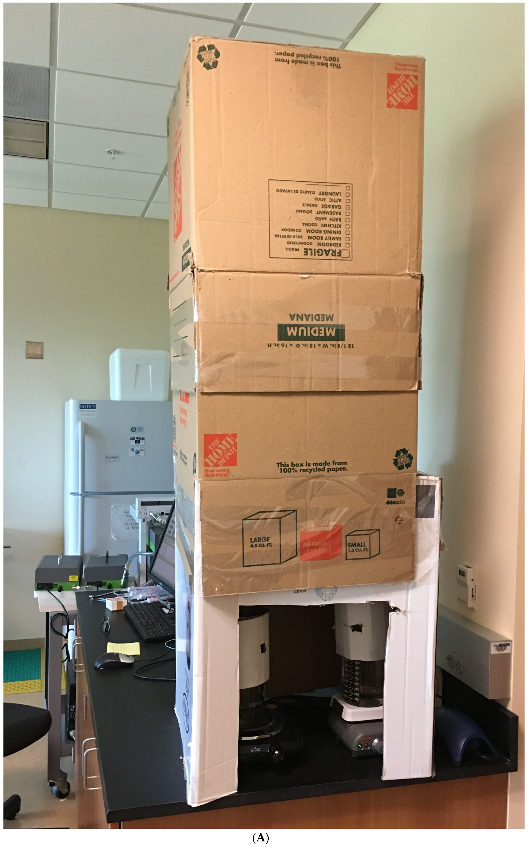
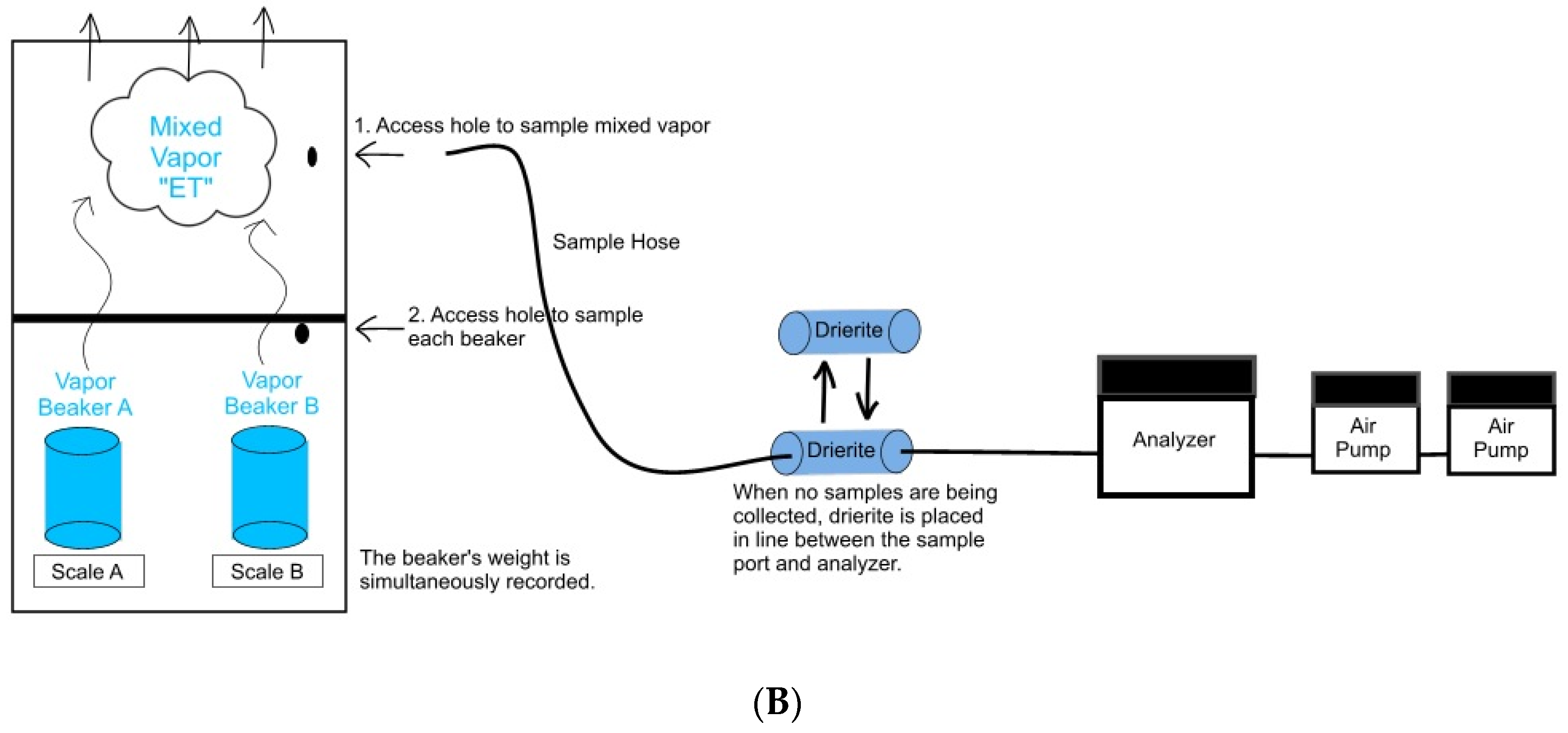
A collar was attached to each beaker to isolate its vapors and the beakers were then placed on hot plates to increase evaporation rates. Beaker A was heated to 50 °C and Beaker B was warmed to 30 °C. Vapor samples were collected at 2 elevations. The lower elevation was 5 mm above the liquid layer interface in beakers A and B; this sample point represented the base of the turbulent transport layer. The upper elevation was 60 cm above beakers A and B; this sample point represented the mixed vapor sample in the turbulent transport layer (Figure 1A,B). The vapor samples were collected directly in the Picarro L2130 Water Isotope Analyzer through a short sample hose that fed directly into the instrument. Vapor was sampled at each location for at least 5 min or until the water-vapor concentration exceeded a minimum threshold of 15,000 parts per million (ppm). Collection of the 3 vapor samples constituted a cycle; at the end of each cycle, 2 mL of water was removed by syringe from each beaker and stored in 2 mL autosampler borosilicate glass vials, without headspace. Vials were capped and stored in the laboratory for later isotope analysis, and not used in the scope of this study. Each experiment included 2 to 6 cycles. A total of 3 separate experiments were performed in the laboratory. Between the collection of each sample, a container pack filled with Drierite was placed in line with the sample hose to reduce water vapor inside the sample tubing and to reduce the water-vapor concentration inside the Cavity Ring-Down Spectrometer chamber to 1000 ppm.
2.2. Field Water-Vapor Isotopic Sampling
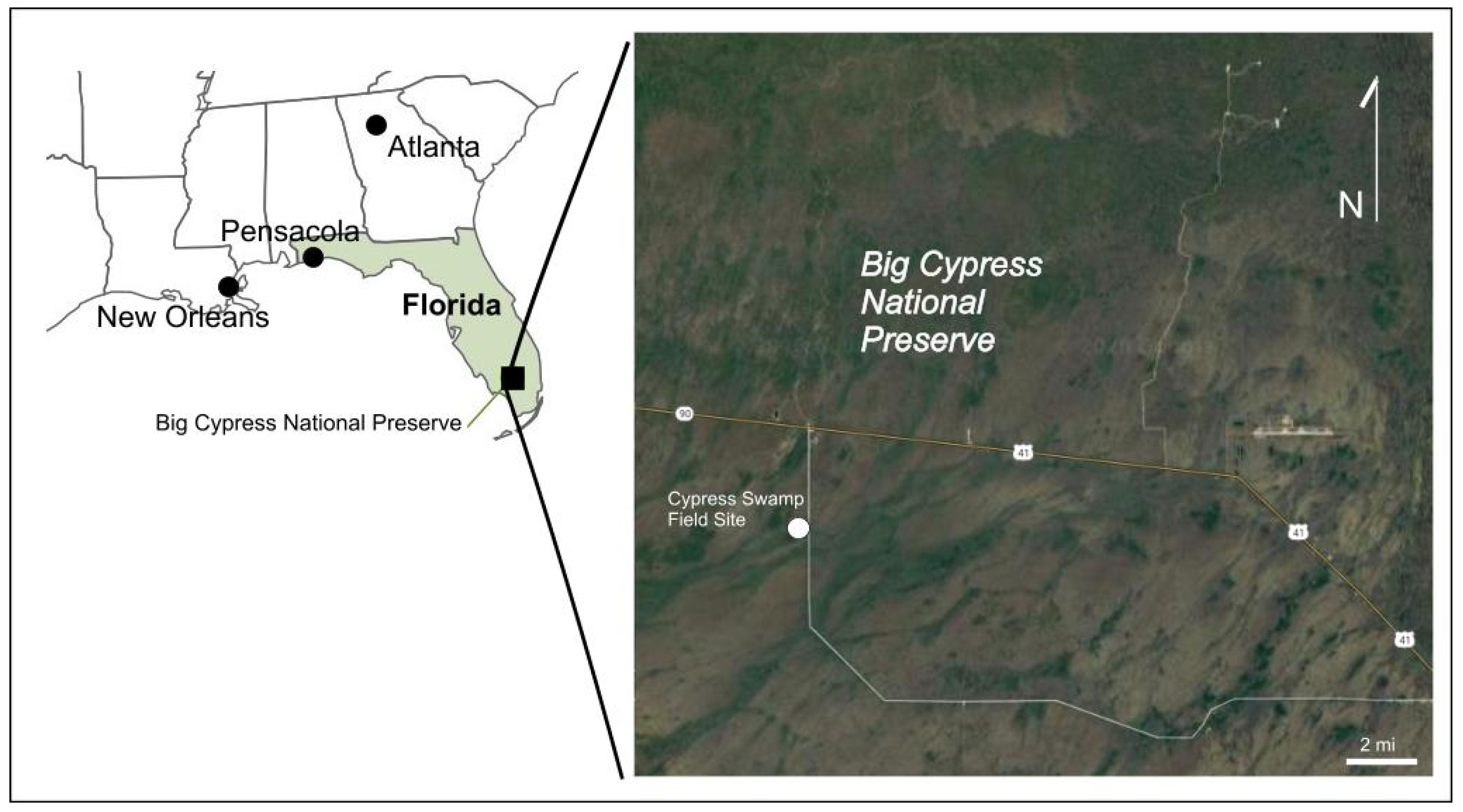
The experimental method developed in the lab was applied to the field data collected at the Cypress Swamp site in the Big Cypress National Preserve (BCNP), Florida (25.82207 N, 81.101689 W), Figure 2.
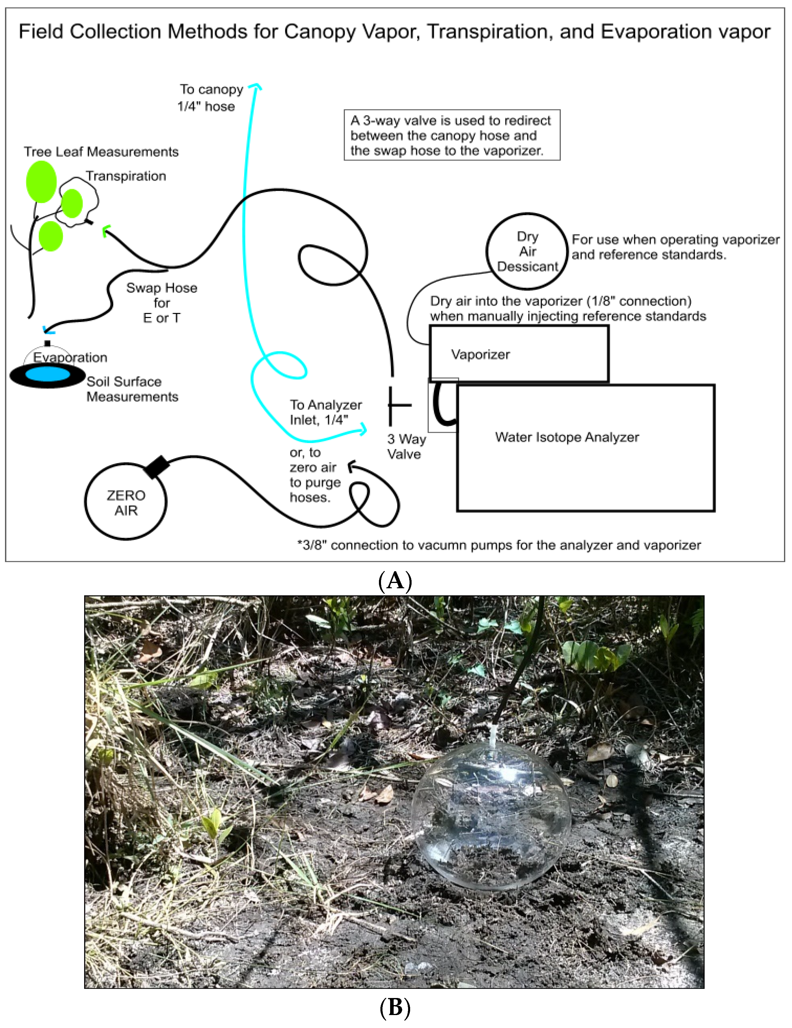
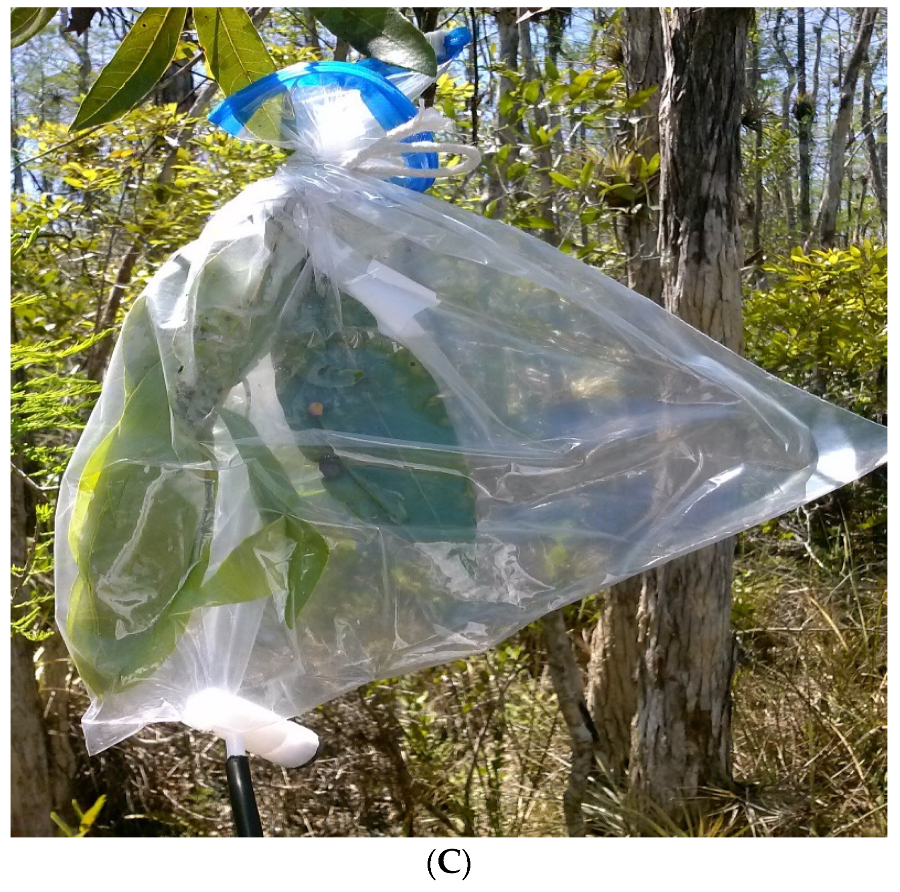
The area classification was a swamp forest with tall, dense cypress trees and a subcanopy of mixed hardwoods, Shoemaker, W. B., et al., 2011 [10]. Air samples for isotopic analysis were collected from 3 distinct sources (Figure 3A). Evaporation source vapors (δE) were sampled from the forest floor. Soil air, which represented, δE was collected using a 6-inch diameter sphere halved and outfitted with a sample hose at the top that fed directly into the Picarro L2130 Water Isotope Analyzer, (Figure 3B). Air surrounding the leaves represented transpiration source vapors (δT) and was collected using a clear Ziploc® (Racine, WI, USA) bag. The clear bag enveloped the leaves and was sealed by a string tied to the branch. The clear bag allowed for photosynthesis to occur uninterrupted. A sample hose fed directly into the analyzer from the bag (Figure 3C). The third sample corresponding to ET was collected at the top of a USGS microclimate station tower adjacent to the eddy flux sensors about 36 m above the land surface. The canopy source vapors (δET) were fed directly into the analyzer via a sample hose, (Figure 3A). From the morning at 10 AM through to the afternoon at 4 PM, the experiment was repeated 4 times following the aforementioned procedures. Before and after sampling, reference samples USGS45, W67400, and USGS48 were run through the isotopic analyzer for correction and calibrations using the same methods as those in the lab.
2.3. EC Flux Data Sampling
At the Big Cypress field site, the USGS maintains an adjacent flux station. EC instrumentation for data collection included a 10 Hz, 3-dimensional sonic anemometer for measuring wind velocities, and a gas analyzer for measuring water-vapor concentrations [8]. Other instruments included a pyranometer, net radiometers, soil heat flux plates, and relative humidity and temperature probes. These are all essential tools for measuring eddy fluxes for trace gases and applying the necessary corrections [8,9]. The EC Flux record use is discussed in (Section 5.5).
3. Post-Sampling Data Processing
3.1. Data Screening, Instrument Drift Correction, and Data Calibration
Gupta, P. et al., 2009, consider isotope data of 18O, with a standard deviation of 0.2 per mil (‰) or less, as stable [11]. To determine which laboratory measurements are most stable, the standard deviation of the isotope data was calculated at 1-min intervals using the Microsoft Excel statistical functions software package. 18O/16O isotope ratios with standard deviations of 0.2 per mil (‰) or less were selected for further calibration and finalizing. Generally, the most stable isotope data occurred within 3 to 5 min of a sampling cycle. Briefly, systems that use liquid injection via a vaporizer module are prone to memory effects, i.e., the carry-over from the previously analyzed sample in a sequence generally overestimates isotopic values [12]. Optimization methods reported by Geldern, R. and Barth J. A. (2012) were applied to the isotope liquid and vapor measurements for instrument drift corrections and calibrations. Observations of each unknown vapor were made, and measurements of USGS and Laboratory reference waters (W-67400: +1.2‰, −1.97‰; USGS 45: −10.3‰, −2.238‰; USGS 48: −2.0‰, −2.224‰; Lab 001: +6.08‰, + 0.24‰; Lab 002: −55.34‰, −7.45‰; for H and O, respectively) as part of each experiment were used to correct raw data for sample-to-sample memory effects and instrument drift corrections. Observations from each experiment were averaged to obtain uncalibrated sample values. USGS and Laboratory reference values were used to calibrate sample values to the VSMOW-SLAP reference scale using a three-point laboratory or two-point field linear calibration. [12]. The reproducibility of replicate standards varied from 0.01‰ to −0.92‰ for oxygen and −0.02‰ and −13.9‰ for hydrogen. Similar variations are reported in Geldern, R. and Barth J. A., (2012), Gupta, P. et al., 2009, and Tremoy, G. et al., 2011 [11,12,13].
3.2. Partitioning of Water-Vapor Sources Using the Isotope Mass Balance
An isotope mass balance equation (IMB) was used to determine the isotopic compositions from Beakers A, (light) and B, (heavy), and the resulting mixed vapor above the beakers. Yakir, D., and da SL Sternberg, L., 2000 presented a basic equation for a two-source mixing model that quantifies the fractional contribution of each source to the mixed vapor [14]. The estimates were obtained from the individual water-vapor observations.
where Fb (%) is the fractional contribution by Beaker B, (heavy) to the total mixed vapor, and δmixed, δa, and δb are the isotopic compositions of the mixed vapor above the beakers, Beaker A, (light) vapor source and Beaker B, (heavy) vapor source, respectively. For clarity, Fb (%), δa, and δb are substituted for , and A similar arrangement can be made for the fractional contribution from Beaker A, (light):
where
where is the fractional contribution by Beaker A, (light) to the total mixed vapor. The δmixed, δa, and δb are the isotopic compositions of the mixed vapor above the beakers, Beaker A, (light) vapor source and Beaker B, (heavy) vapor source, respectively. For clarity, , δa, and δb are substituted for , and The above equations can be solved using either δ18O or δ2H to determine the percentage contribution of each source to the mixed vapor.
3.3. Model Verification Using the Mass Balance Technique
The beaker weights were simultaneously recorded, and these weights were determined with a precision of 0.0001 g. The mass of water that evaporated from each beaker was calculated as each vapor was sampled. A water mass balance approach was used to determine the percent contribution from each beaker to the mixed vapor.
where
MT = BA + BB,
Percent of BA to MT total contribution (M1) = BA/MT × 100,
Percent of BB to MT total contribution (M2) = BB/MT × 100,
MT = Total Mass of Water Evaporated,
BA = Mass of water evaporated from Beaker A,
BB = Mass of water evaporated from Beaker B,
For example, if the IMB fractional contribution of water evaporated from Beaker A is equal to 50%, then the water mass balance of Beaker A should be 50%. The IMB reflects the water mass balance.
4. Results
4.1. Mass Balance Partitioning in the Laboratory
The isotope partitioning method was applied to the calibrated vapor sources to determine individual δ2H and δ18O compositions. The results provide a comparison between isotope mass balance ratios and water mass balance ratios. Beakers with the highest ratio illustrate which beaker has the highest evaporation rate and contributes to the largest amount of water vapor to the mixed vapor above.
In the first lab experiment, Beaker A δ18O values ranged from −7.53 per mil (‰) to −7.69‰. Beaker B δ2H‰ ranged from −5.65‰ to −5.32‰, Mixed Vapor ranged from −5.77‰ to −5.80‰. Beaker A (Light) values of δ2H‰ ranged from −79.59‰ to −92.10‰, Beaker B (Heavy) ranged from −83.52‰ to −84.52‰, and Mixed Vapor ranged from −84.14‰ to −84.16‰. Values of δ18O in the water sources ranged from −1.49‰ to 6.09‰; values of δ2H‰ ranged from −3.02‰ to 25.18‰. The average isotope mass ratio of beaker vapors in the two trials was from 0.13 to 0.87. The contents of Beaker B contributed more to the mixed vapor. The water mass balance ratio was from 0.32 to 0.68; its ratio differed from the δ18O IMB by 0.16 or 16%.
The second experiment contained three cycles. Beaker A δ18O values ranged from −13.48‰ to −15.01‰, Beaker B δ18O values ranged from −5.65‰ to −5.32‰, Mixed Vapor δ18O ranged from −5.77‰ to −5.80‰. Beaker A values of δ2H‰ ranged from −79.59‰ to −92.10‰, Beaker B δ2H ranged from −83.52‰ to −84.52‰, and Mixed Vapor δ2H ranged from −84.14‰ to −84.16‰ were recorded. Values of δ18O in the water sources were between −1.28‰ and 6.61‰; values of δ2H ‰ were between −3.61‰ and 19.19. The average isotopic mass ratio of vapors in each beaker was 0.68 and 0.32. Beaker A’s water balance ratio ranged from 0.67 to 0.33 and made a greater contribution to the mixed vapor. This ratio differed in that it was 0.09 or 9% larger than δ18O IMB.
The third experiment comprised three cycles. Beaker A δ18O values ranged from −15.67‰ to −15.97‰, Beaker B δ18O values ranged from −13.39‰ to −15.13‰, Mixed Vapor δ18O values ranged from −14.89‰ to −15.44‰. Beaker A values of δ2H‰ ranged from −157.93‰ to −170.06‰, Beaker B δ2H‰ ranged from −156.03‰ to −158.88‰, and Mixed Vapor δ2H‰ ranged from −160.75‰ to −164.16‰. Values of δ18O in the water sources ranged from 0.38‰ to 8.40‰; values of δ2H ranged from −0.19‰ to 29.95‰. The average δ18O isotope mass ratio in each beaker was 0.25 in Beaker A and 0.75 in Beaker B. Beaker B contributed more to the mixed vapor. The water balance ratio, 0.40 to 0.60, differed from the δ18O IMB by 0.15 or 15%.
4.2. Mass Balance Partioning in Big Cypress, Florida
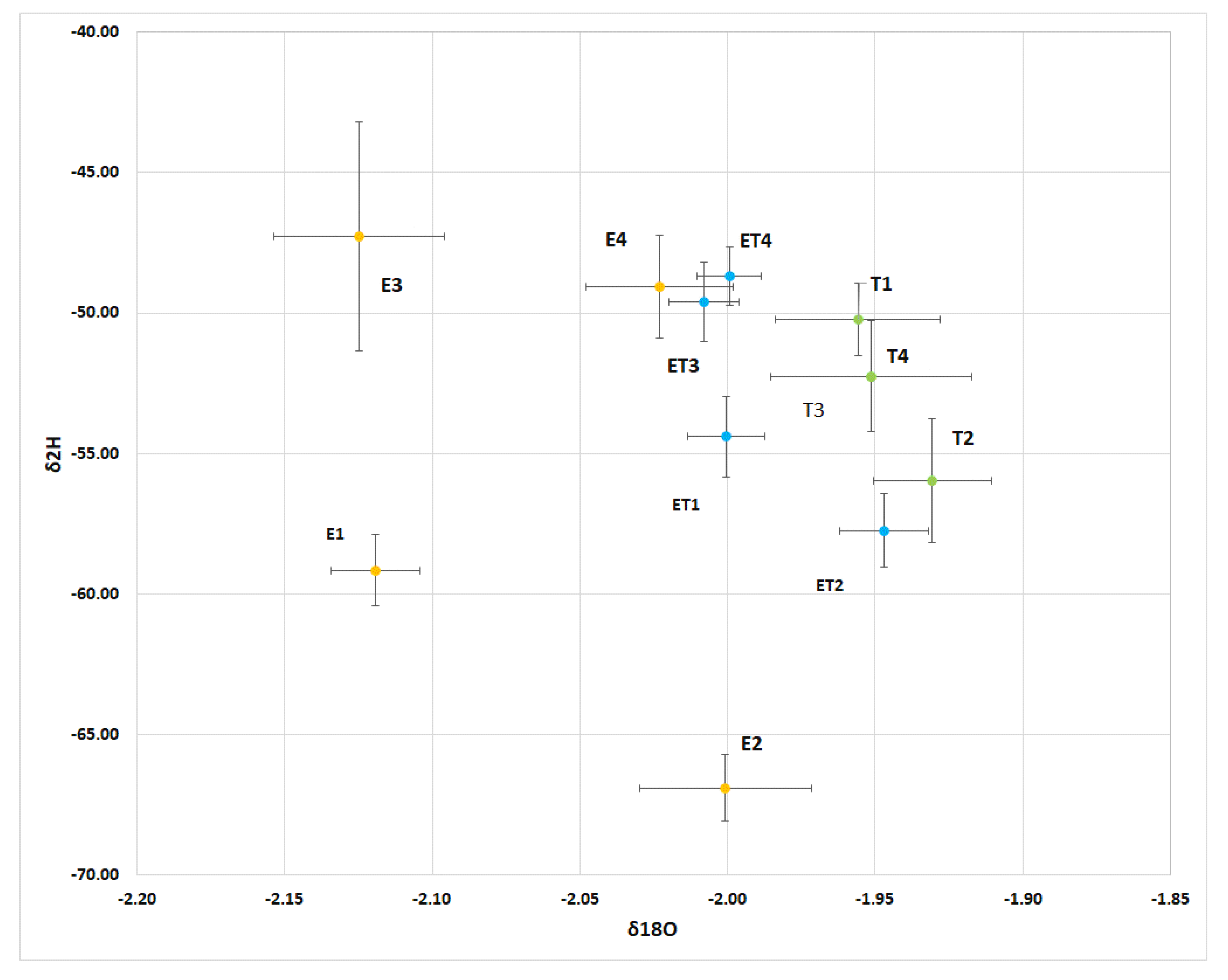
The field experiment took place on 2 April 2014. It was a sunny day with low humidity and cool weather for Big Cypress, Florida. Temperatures ranged between the low 10’s to 25 Celsius allowing for several water vapor observations to be completed. Observations at 10:47 and 12:09 were poor measurements. Due to cloud cover, the observations 14:58 and 15:08 did not fall between the end members. The observations consisted of four cycles. The δ18O values of evaporation source vapor (δE) were between −2.00‰ and −2.12‰, whereas δ2H values of evaporation source vapors (δE) ranged between −47.26‰ and −66.90‰. δ18O values of transpiration source vapors (δT) ranged between −1.93‰ and −2.04‰. δ2H values of transpiration source vapors (δT) ranged between −41.55‰ and −68.35‰. δ18O values of the canopy source vapors (δET) ranged between −1.95‰ and −2.01‰ for δ18O. δ2H values of canopy source vapors (δET) ranged between −44.79‰ and −57.75 ‰. Table 2 presents the observations from the Big Cypress field experiment and Figure 4 plots the spatial distribution with standard deviations.
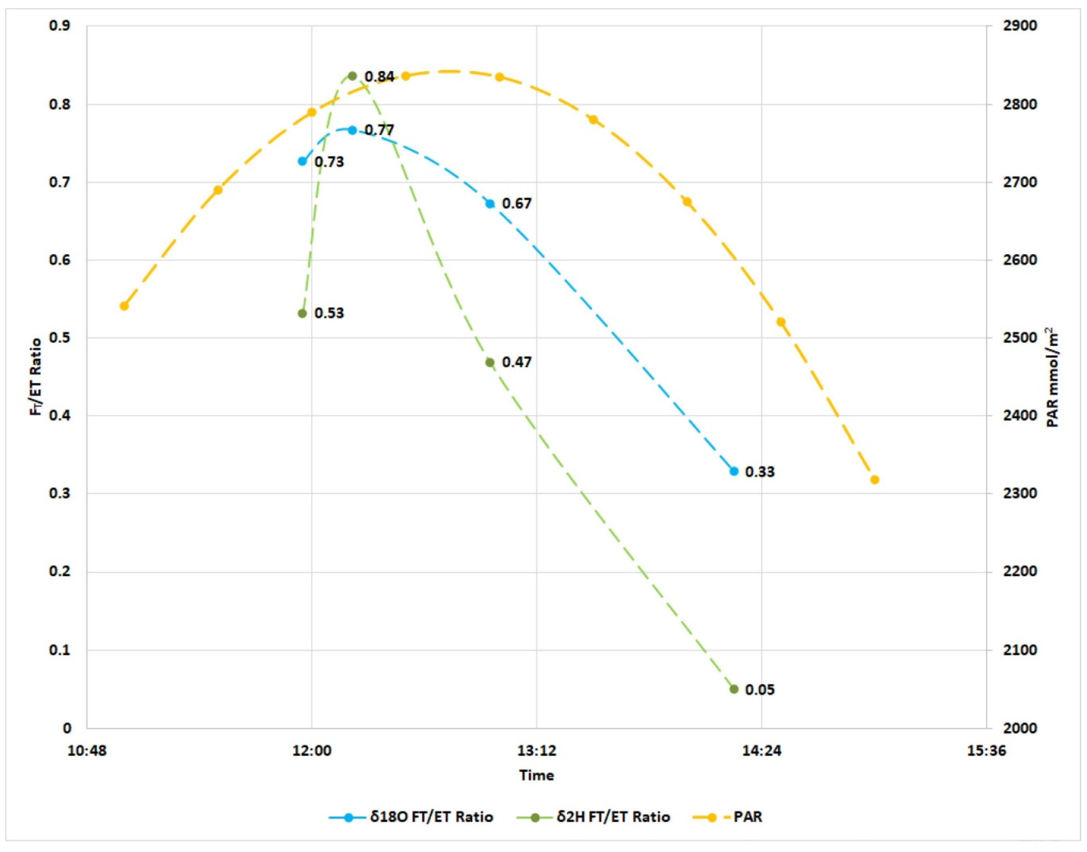
Water-vapor observations were acquired from 10:47 to 15:08 at the field site in Big Cypress, Florida. The range of ratios of transpiration-flux to composite-flux oxygen-18 isotope measurements (FT/ET δ18O) were from 0.33 to 0.77. The range of ratios of evaporation-flux to composite-flux oxygen-18 isotope δ18O, (FE/ET) were from 0.23 to 0.67, (Table 3).
The range of ratios for δ2H FT/ET was from 0.05 to 0.84. The range of ratios for δ2H FE/ET was from 0.16 to 0.95.
The average isotope ratio for δ18O FT/ET was 0.62. The average isotope ratio for δ18O FE/ET was 0.38. Between the two sources measured, the greater contribution to ET was from δ18O FT/ET transpiration-flux. The average isotope ratio for δ2H FT/ET was 0.47, and the average isotope ratio for δ2H FE/ET was 0.53, (Figure 5). δ2H FE/ET had a larger contribution from the evaporation-flux to ET, which dominated due to the shading from cloud cover during the fourth sample cycle. Table 3 presents the ratio calculations from the Big Cypress field experiment. Further discussion on uncertainty is in Section 5.
5. Discussion
5.1. Changing Isotopic Composition by Fractionation
Fractionation processes are well documented by Geldern, R. and Barth, J.A., 2010; Tremov, G. et al., 2011, Yakir, D., and da SL Sternberg, L., 2000; Gaj, M., et al., 2016, Kool et al., 2014, and Gat, J. 2010 [12,13,14,15,16,17]. In this set of experiments, the vapor measurements are collected within relatively high humid settings resulting in temperature and humidity dominating the nonequilibrium fractionation processes. Depletion effects can contribute as much as an order of magnitude of variability between the δ2H and δ18O measurements [17].
Vapor measurements can have lengthy observation times. Due to tubing materials and long lengths, Tremov, G. et al., 2011 suggest that isotopic composition can experience depletion, as measured by low δ2H measurements [13].
5.2. The Significance of the Results
Spectroscopic methods for simultaneously measuring gases, including water vapor, will continue to improve. This technique allows for the direct observation of water-vapor isotopes [11]. The experiments show how to measure the isotopic composition of mixed water vapor accurately in a controlled setting. Favorable agreement of the laboratory results compared with highly accurate water mass balance (WMB) measurements illustrate that the IMB method can be a rapid ET partitioning tool. The uncertainty for these experiments averages less than 20% and is within other ET methods for estimation and partitioning [11,16]. Parameters known to contribute to uncertainty are d-excess, humidity, and temperature. They are rapidly quantifiable and will eventually be corrected in situ.
The performance of the IMB method will depend on land cover. Humid environments such as South Florida have shallow water tables, thus a small separation between groundwater and soil moisture isotopic sources. During some wet seasons, the ET end members will possibly overlap.
5.3. Uncertainty in the Measurements
Attempts to directly measure water-vapor isotopes may lead to numerous discrepancies. The natural environment is not a static regime. It contains a considerable number of variable sources. As direct meteorological measurements show, the attributes contributing to the isotopic composition of water vapor are always in flux. For example, changes in temperature, cloud cover, air pressure, relative humidity, evaporation, and condensation contribute to the isotope fractionation processes.
It is essential to understand the isotopic compositional limits of the ecosystem [20]. There is no substitute for understanding the dynamics of the study site. Measurements during all seasons will help reduce both underestimation and overestimation of isotopic compositions.
The methods themselves can influence the isotopic composition measured. Even in a controlled lab setting, maintaining spatiotemporal conditions are equally as important as in the field. When one makes observations of water vapor, the measurements at a liquid surface in the turbulent layer are susceptible to changing environmental conditions such as temperature and relative humidity. Circumstances that will change the equilibrium isotope factors are critical for modeling isotope fractionation activity within the liquid and vapor phases. Conceived initially by Majoube, M., 1971 [21] and later improved by Horita, J., and Wesolowski, D. J., 1994 [22] and Fang, G., and Ward, C. A., 1999 [23], the isotope fractionation equilibrium model is used to quantify evaporation [20,21,22].
To further emphasize, Swain, E., and Decker, J., (2010) studied evaporation using water tanks altered to simulate wetland temperature conditions [24]. They utilized the Clausius–Clapeyron equation to shed light on the exponential relationship between saturation water-vapor pressure and measurement height above an evaporating surface of water. In the context of water isotopes, their results highlight the importance of the isotopic fractionation factor. Water-vapor pressure is a significant contributor to the fractionation effects of water isotopes. Samples taken at different heights above the evaporated surface will yield various isotopic water-vapor compositions. Lack of consistency in measurements of beaker observation height, soil floor, and distance from canopy can all strongly influence the variation in isotope composition; such variation can lead to less accurate δ18O and δ2H end-member measurements.
Poor observations can come from a variety of causes,
- inconsistent distances from the evaporating surface,
- tubing effects,
- different temperatures,
- relative humidity,
- varying vapor pressures,
are all factors that can enrich or deplete the isotopic compositions. The uncertainties can be systematic enough to affect observations significantly or become more or less prominent than end member observations.
5.4. ET Ratios of This Study and Similar Studies
For many decades, water isotope studies have successfully determined water contributions in nearly all parts of the hydrologic cycle. However, only recently, with the increasing awareness of water scarcity, ET partitioning studies have grown rapidly in number. The many methods used in such studies (such as cryogenic vacuum devices, lysimeters, Sap Flow instruments, and the Bowen Ratio Energy Balance method) have directly or indirectly estimated evapotranspiration and its components. These methods typically provide accurate point data. To highlight the accuracy of the results, comparisons with ET partition studies set in natural settings are described below.
In Northern European forests, studies employed direct methods using microlysimeters and soil chambers to estimate E/ET ratios between 0.05 to 0.15 [25]. Sap Flow methods estimated T/ET ratios from 0.85 to 0.95 [25]. In Southern Israel, a direct approach using soil chambers produced estimates of E/ET ratios of 0.33 to 0.42 [26]. Using Sap Flow methods, the estimates of T/ET ratios ranged from 0.44 to 0.57 [26]. In these two locations (Northern Europe and Israel), the ratios of E/ET differ. The ratio of E/ET in Israel is higher than those of Northern Europe because the latitude of Israel receives a higher amount of direct solar radiation than Northern Europe.
In forested Southern Angola and Northern Namibia, Gaj et al., 2016, produced a soil-water balance along with precipitation, recharge, soil-water storage, and runoff [15]. Cryogenic methods were used to capture soil water and provide a soil-moisture depth profile to estimate the evaporation front. Observations of groundwater storage, evaporation, and runoff are subtracted from precipitation in the water balance equation; an estimate of the ratio of transpiration to total evapotranspiration (T/ET) was from 0.75 to 0.78 [15]. This range of values depends on soil moisture conditions and can be higher in nonvegetated areas.
In a similar natural Southeastern Arizona shrub setting, Stannard, D. I., and Weltz, M. A., utilized a chamber method approach to produce estimates of ET partitions from 0.16 E/ET and 0.84 T/ET [27]. Total ET was determined using an eddy correlation (also known as eddy covariance) method without Bowen’s ratio correction. The ET ratio between the two approaches (E + T/ET) is 1.26, (See Table 4).
The summary of land-covers and ET partition results described above compare with the Big Cypress field setting. Direct methods for measuring transpiration show a similar dominant contribution to ET, Kool et al., 2014, Köstner, B., 2001, Yaseef, N., et al., 2012, Scott R. L. et al., 2006, Stannard, D. I., and Weltz, M. A., 2006 [16,25,26,27,28]. In Table 4, the compared Big Cypress field results agree with the observations.
5.5. Comparison between Field Isotopic Mass Balance and the Flux Variance Similarity Partitioning Ratios
The Flux Variance Similarity (FVS) method is based on transport-derived scalars of high-frequency water vapor and carbon dioxide taken from a single point [29,30]. The changes in water-vapor concentration are divided into constituents driven by stomatal (transpiration) and nonstomatal (evaporation) factors. Changes in carbon dioxide concentration are driven by nonstomatal (respiration) and stomatal (photosynthesis) factors. The result is a nonlinear two-equation system that must be solved algebraically.
Just as EC methods require satisfactory meteorological conditions for proper ET flux estimations, so does the FVS method. It needs a similar set of meteorological conditions to be reliable. For example, in early daylight hours, laminar airflow may be incompatible with the theory or assumptions, resulting in data gaps [8,9,10,30].
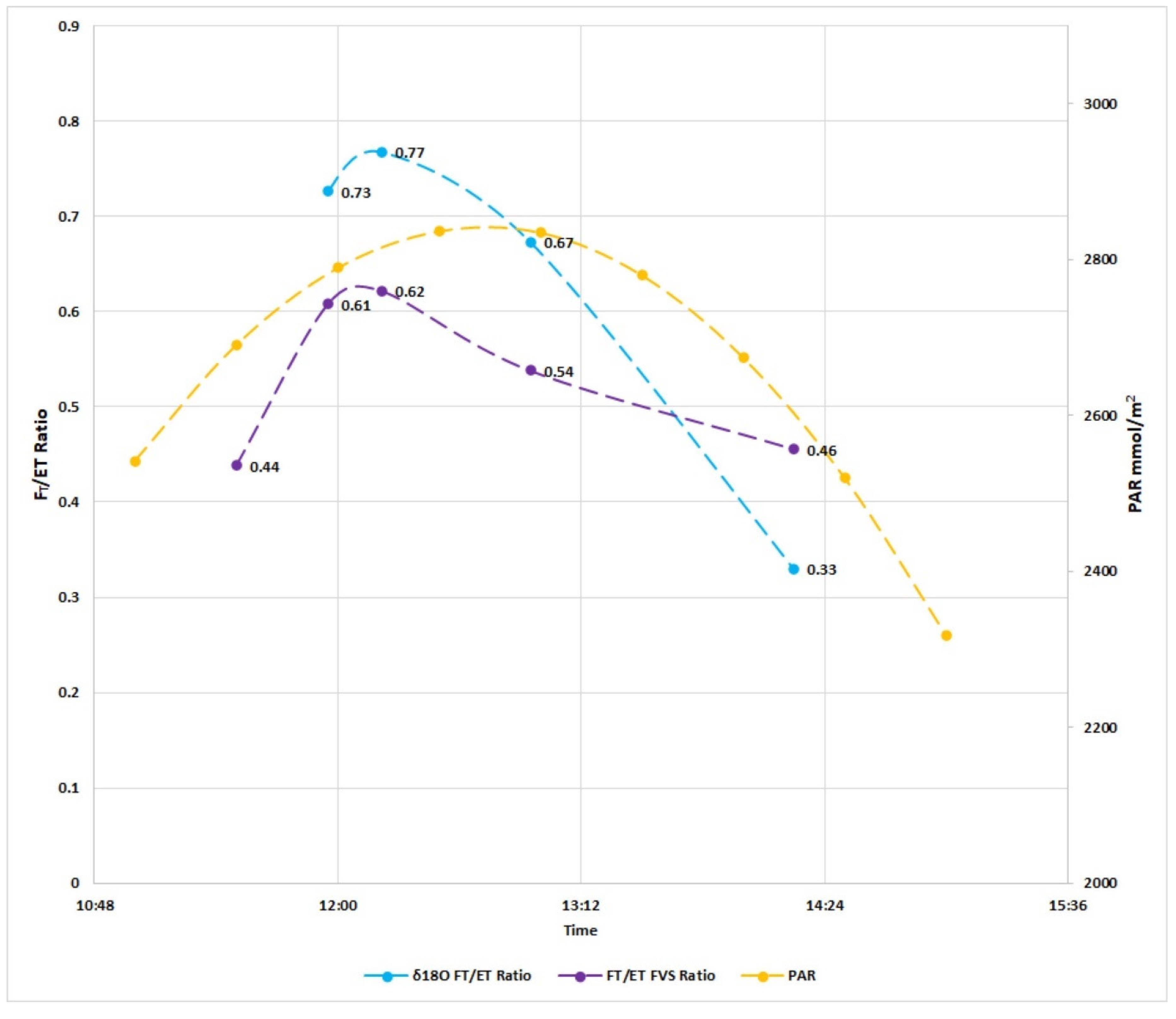
Fluxpart is a program that can be used to apply the FVS method. It is an open-source Python 3 program that can utilize metadata and raw 10 Hz EC data to produce ET and CO2 partitions and fluxes at 15 min intervals. The Big Cypress field site was the same location as that used for the field isotope data collection. Furthermore, 10 Hz high-resolution EC data from the Big Cypress microclimate flux station, measured on the same day as the Isotope observations, were used as the input data to run the Fluxpart program. For related timeframes, a comparison between the FVS and IMB results are presented below, (Figure 6).
The FT/ET ratios differed by 12% to 7% between the IMB O18 and FVS methods. The standard deviation was 0.34 for the IMB and 0.19 for the FVS values. FVS and IMB use different methods to produce results. Comparisons between FVS and IMB partitions (ratios) are in agreement.
The Ft/ET ratio ranges demonstrated differences of 35% to 7% between IMB H2 and FVS. The standard deviation for FVS was 0.19 and 0.34 for the IMB ratio. The FVS ratios are in agreement with the IMB field data ratios. The results illustrate that the IMB methods can partition ET into evaporation and transpiration components (Table 5).
6. Conclusions
It has been determined that water vapor isotopes can be used to quantify independent evaporation and transpiration sources. Although this IMB approach is noteworthy, measuring water-vapor isotopes is a complicated task. Additional research is recommended for the detection and measurement of ambient water-vapor source contributions. The experiments explore a rapid deployable method for measuring individual water vapor sources and a tool for partitioning ET into its end members.
The experiments highlighted considerable isotopic variability from the methods employed. Comparing the IMB to very accurate WMB, the measurement uncertainty is quantifiable. A reduction in the uncertainty is possible in water vapor measurements by controlling or measuring those parameters that need to be resolved either as part of the calibration process or applied as a correction to the observations in-situ.
Comparing the field results to other studies with similar land cover revealed the dominance of vegetation contribution to the ET flux. Adaptations to the IMB results aid in qualifying or ranking isotopic sources [17,31,32]. IMB application improvements could help refine the accuracy and prediction ability of isotope-enabled atmospheric general circulation models [33]. The coupling of tropospheric vapor pathways to atmospheric circulation is essential for understanding the hydrologic cycle [34,35].
Additionally, validating the IMB method with the FVS method gave additional confirmation, and it also presents an example for upscaling ET to larger footprints. In this case, we could apply the ratios to the fluxes determined by EC methods. The partition ratio can also be applied to satellite ET derived results or conventional methods used for ET estimation [36].
This paper illustrated that it is possible to derive components from sources of different isotopic compositions accurately. The result shows that it is possible to use IMB ET ratios across different scales. IMB results are valuable. Combined with other ET methods, the results can provide calibration to remotely sensed regional ET estimates [36]. The ET scaled estimations preserve their accuracy and compare well with other methods. With an improved temporal resolution and a more extended time series, IMB assessments can further our understanding of ET dynamics at the terrestrial source.
Funding
This research was funded by H2OResource, Inc., the Florida Atlantic University GRIP grant program, the FAU Department of Geosciences, University of Florida, Institute of Food and Agricultural Sciences, Ft. Lauderdale, and the USGS Ft. Lauderdale Water Science Center.
Acknowledgments
I would like to thank the following for helping to support this project: Former geology students, Augustine Alvarez, Alexander Garcia, Erica Dubouff, and Mario Job. Florida Atlantic University GRIP grant program and the Department of Geosciences; University of Florida IFAS Ft. Lauderdale; the U.S. Geological Survey Ft. Lauderdale Water Science Center; five anonymous reviewers; Byron Winston, Dane Elliot-Lewis, and Mary-Margaret Coates for their constructive and thoughtful comments; and John Leftwich for helping me stay the course. Peter Morris, Distributed Technologies (UK) Ltd. for assistance with the Python coding and Todd Skaggs for his unwavering support. I also thank Jiahong Li and George Burba for teaching me about the numbers hidden in the flux. Thank you to the folks at Picarro, Danthu Vu, Kate Dennis and David Kim-Hak for your technical support and patience. Most of all, thanks to USGS Scientists Barclay Shoemaker and David Sumner for giving me the opportunity to get back into the geosciences.
Conflicts of Interest
The author declares no conflict of interest.
References
- Farquhar, G.D.; Cernusak, L.A.; Barnes, B. Heavy water fractionation during transpiration. Plant Physiol. 2007, 143, 11–18. [Google Scholar] [CrossRef] [PubMed] [Green Version]
- Wenninger, J.; Beza, D.T.; Uhlenbrook, S. Experimental investigations of water fluxes within the soil–vegetation–atmosphere system: Stable isotope mass-balance approach to partition evaporation and transpiration. Phys. Chem. Earthparts A/B/C 2010, 35, 565–570. [Google Scholar] [CrossRef]
- Good, S.P.; Mallia, D.V.; Lin, J.C.; Bowen, G.J. Stable isotope analysis of precipitation samples obtained via crowdsourcing reveals the spatiotemporal evolution of superstorm sandy. PLoS ONE 2014, 9, e91117. [Google Scholar] [CrossRef] [PubMed] [Green Version]
- Zhang, S.; Wen, X.; Wang, J.; Yu, G.; Sun, X. The use of stable isotopes to partition evapotranspiration fluxes into evaporation and transpiration. Acta Ecol. Sin. 2010, 30, 201–209. [Google Scholar] [CrossRef]
- Li, G.; Li, B. Isotope mass balance method to partition evaporation and transpiration in cropping field. IAEA Tecdoc. Ser. 2017, 75–82. Available online: https://www-pub.iaea.org/MTCD/Publications/PDF/TE-1813_web.pdf#page=84 (accessed on 9 November 2019).
- Talsma, C.; Good, S.; Miralles, D.; Fisher, J.; Martens, B.; Jimenez, C.; Purdy, A. Sensitivity of Evapotranspiration Components in Remote Sensing-Based Models. Remote Sens. 2018, 10, 1601. [Google Scholar] [CrossRef] [Green Version]
- Urbina, C.A.; van Dam, J.C.; Hendriks, R.F.A.; van den Berg, F.; Gooren, H.P.A.; Ritsema, C.J. Water flow in soils with heterogeneous macropore geometries. Vadose Zone J. 2019, 18, 1–17. [Google Scholar] [CrossRef]
- Baldocchi, D.D.; Hincks, B.B.; Meyers, T.P. Measuring biosphere-atmosphere exchanges of biologically related gases with micrometeorological methods. Ecology 1988, 69, 1331–1340. [Google Scholar] [CrossRef]
- Migliaccio, K.W.; Barclay Shoemaker, W. Estimation of urban subtropical bahiagrass (Paspalum notatum) evapotranspiration using crop coefficients and the eddy covariance method. Hydrol. Process. 2014, 28, 4487–4495. [Google Scholar] [CrossRef]
- Shoemaker, W.B.; Lopez, C.D.; Duever, M.J. Evapotranspiration over spatially extensive plant communities in the Big Cypress National Preserve, southern Florida, 2007–2010. U.S. Geol. Surv. Sci. Invest. Rep. 2011, 5212, 46. [Google Scholar]
- Gupta, P.; Noone, D.; Galewsky, J.; Sweeney, C.; Vaughn, B.H. Demonstration of high-precision continuous measurements of water vapor isotopologues in laboratory and remote field deployments using wavelength-scanned cavity ring-down spectroscopy (WS-CRDS) technology. Rapid Commun. Mass Spectrom. 2009, 23, 2534–2542. [Google Scholar] [CrossRef] [PubMed]
- Geldern, R.; Barth, J.A. Optimization of instrument setup and post-run corrections for oxygen and hydrogen stable isotope measurements of water by isotope ratio infrared spectroscopy (IRIS). Limnol. Oceanogr. Methods 2012, 10, 1024–1036. [Google Scholar] [CrossRef]
- Tremoy, G.; Vimeux, F.; Cattani, O.; Mayaki, S.; Souley, I.; Favreau, G. Measurements of water vapor isotope ratios with wavelength-scanned cavity ring-down spectroscopy technology: New insights and important caveats for deuterium excess measurements in tropical areas in comparison with isotope-ratio mass spectrometry. Rapid Commun. Mass Spectrom. 2011, 25, 3469–3480. [Google Scholar] [CrossRef] [PubMed]
- Yakir, D.; da SL Sternberg, L. The use of stable isotopes to study ecosystem gas exchange. Oecologia 2000, 123, 297–311. [Google Scholar] [CrossRef] [PubMed]
- Gaj, M.; Beyer, M.; Koeniger, P.; Wanke, H.; Hamutoko, J.; Himmelsbach, T. In situ unsaturated zone water stable isotope (2H and 18O) measurements in semi-arid environments: A soil water balance. Hydrol. Earth Syst. Sci. 2016, 20, 715–731. [Google Scholar] [CrossRef] [Green Version]
- Kool, D.; Agam, N.; Lazarovitch, N.; Heitman, J.L.; Sauer, T.J.; Ben-Gal, A. A review of approaches for evapotranspiration partitioning. Agric. Meteorol. 2014, 184, 56–70. [Google Scholar] [CrossRef]
- Gat, J. Isotope Hydrology: A Study of the Water Cycle; Imperial College Press, World Scientific: Singapore, 2010; Volume 6. [Google Scholar]
- Clark, I.D.; Fritz, P. Environmental Isotopes in Hydrogeology; CRC Press: Boca Raton, FL, USA, 2013. [Google Scholar]
- Sutanto, S.J.; Van den Hurk, G.B.; Hoffmann, J.; Wenninger, P.A.; Dirmeyer, S.I.; Seneviratne, T.; Röckmann, K.E.; Trenberth, E.; Blyth, M. HESS Opinions “A perspective on isotope versus non-isotope approaches to determine the contribution of transpiration to total evaporation”. Hydrol. Earth Syst. Sci. 2014, 18, 2815–2827. [Google Scholar] [CrossRef] [Green Version]
- Craig, H.; Gordon, L.I. Deuterium and oxygen 18 variations in the ocean and the marine atmosphere. In Stable Isotopes in Oceanographic Studies and Paleotemperatures; Consiglio Nazionale Delle Ricerche Laboratorio Di Geologia Nucleare—Pisa: Spoleto, Italy, 1965; pp. 9–130. [Google Scholar]
- Majoube, M. Fractionnement en oxygene 18 et en deuterium entre l’eau et sa vapeur. J. De Chim. Phys. 1971, 68, 1423–1436. [Google Scholar] [CrossRef]
- Horita, J.; Wesolowski, D.J. Liquid-vapor fractionation of oxygen and hydrogen isotopes of water from the freezing to the critical temperature. Geochim. Et Cosmochim. Acta 1994, 58, 3425–3437. [Google Scholar] [CrossRef]
- Fang, G.; Ward, C.A. Temperature measured close to the interface of an evaporating liquid. Phys. Rev. E 1999, 59, 417–428. [Google Scholar] [CrossRef]
- Swain, E.; Decker, J. Measurement-derived Heat-budget Approaches for Simulating Coastal Wetland Temperature with a Hydrodynamic Model. Wetlands 2010, 30, 635–648. [Google Scholar] [CrossRef]
- Köstner, B. Evaporation and transpiration from forests in Central Europe–relevance of patch-level studies for spatial scaling. Meteorol. Atmos. Phys. 2001, 76, 69–82. [Google Scholar] [CrossRef]
- Raz-Yaseef, N.; Yakir, D.; Schiller, G.; Cohen, S. Dynamics of evapotranspiration partitioning in a semi-arid forest as affected by temporal rainfall patterns. Agric. For. Meteorol. 2012, 157, 77–85. [Google Scholar] [CrossRef]
- Scott, R.L.; Huxman, T.E.; Cable, W.L.; Emmerich, W.E. Partitioning of evapotranspiration and its relation to carbon dioxide exchange in a Chihuahuan Desert shrubland. Hydrol. Process. 2006, 20, 3227–3243. [Google Scholar] [CrossRef] [Green Version]
- Stannard, D.I.; Weltz, M.A. Partitioning evapotranspiration in sparsely vegetated rangeland using a portable chamber. Water Resour. Res. 2006, 42. [Google Scholar] [CrossRef] [Green Version]
- Skaggs, T.H.; Anderson, R.G.; Alfieri, J.G.; Scanlon, T.M.; Kustas, W.P. Fluxpart: Open source software for partitioning carbon dioxide and water vapor fluxes. Agric. For. Meteorol. 2018, 253–254, 218–224. [Google Scholar] [CrossRef]
- Eiko, N.; Mannarella, I.; Ibrom, A.; Aurela, M.; Burba, G.G.; Dengel, S.; Gielen, B. Standardisation of eddy-covariance flux measurements of methane and nitrous oxide. Int. Agrophys. 2018, 32, 517–549. [Google Scholar]
- Scheihing, K.W.; Moya, C.E.; Struck, U.; Lictevout, E.; Tröger, U. Reassessing Hydrological Processes That Control Stable Isotope Tracers in Groundwater of the Atacama Desert (Northern Chile). Hydrology 2017, 5, 3. [Google Scholar] [CrossRef] [Green Version]
- Markland, T.E.; Berne, B.J. Unraveling quantum mechanical effects in water using isotopic fractionation. Proc. Natl. Acad. Sci. USA 2012, 109, 7988–7991. [Google Scholar] [CrossRef] [Green Version]
- Jean-Louis, B.; Behrens, M.; Meyer, H.; Kipfstuhl, S.; Rabe, B.; Schönicke, L.; Steen-Larsen, H.C.; Werner, M. Resolving the controls of water vapour isotopes in the Atlantic sector. Nat. Commun. 2019, 10, 1–10. [Google Scholar]
- Galewsky, J.; Steen-Larsen, H.C.; Field, R.D.; Worden, J.; Risi, C.; Schneider, M. Stable isotopes in atmospheric water vapor and applications to the hydrologic cycle. Rev. Geophys. 2016, 54, 809–865. [Google Scholar] [CrossRef] [PubMed]
- Schneider, M.; Borger, C.; Wiegele, A.; Hase, F.; García, O.E.; Sepúlveda, E.; Werner, M. MUSICA MetOp/IASI {H2O,δD} pair retrieval simulations for validating tropospheric moisture pathways in atmospheric models. Atmos. Meas. Tech. 2017, 10, 507–525. [Google Scholar] [CrossRef] [Green Version]
- Kalua, M.; Rallings, A.M.; Booth, L.; Medellín-Azuara, J.; Carpin, S.; Viers, J.H. sUAS Remote Sensing of Vineyard Evapotranspiration Quantifies Spatiotemporal Uncertainty in Satellite-Borne ET Estimates. Remote Sens. 2020, 12, 3251. [Google Scholar] [CrossRef]
Figure 1.
(A) Photo of lab experiment. (B) Illustration of lab experimentation.


Figure 2.
Site of field experiment.

Figure 3.
(A) Illustration of field experimentation. (B) Evaporation collection dome. (C) Transpiration collection bag.
Figure 3.
(A) Illustration of field experimentation. (B) Evaporation collection dome. (C) Transpiration collection bag.


Figure 4.
Field isotope observations. Each sample and type are labeled numerically for each cycle.

Figure 5.
IMB FT/ET for δ18O and δ2H ratios of transpiration to evapotranspiration.

Figure 6.
Comparison between IMB δ18O and Flux Variance Similarity (FVS) FT/ET.


Table 1.
Isotope (IMB) and water mass balance ratios measured from three laboratory experiments and ratio differences between each water-vapor source.
Table 1.
Isotope (IMB) and water mass balance ratios measured from three laboratory experiments and ratio differences between each water-vapor source.
| δ18O | δ2H | Beaker A | Beaker B | δ18O Percent Difference | ||||
|---|---|---|---|---|---|---|---|---|
| Fa | Fb | Fa | Fb | Ba | Bb | Fa IMB (Ratio) | Fb IMB (Ratio) | |
| Date/ Time | IMB (Ratio) 1 | IMB (Ratio) 2 | IMB (Ratio) 3 | IMB (Ratio) 4 | Water Mass Bal 5 | Water Mass Bal 6 | and Ba Mass Bal (Ratio) 7 | and Bb Mass Bal (Ratio) 8 |
| 5/12 13:21 | 0.06 | 0.94 | 0.07 | 0.93 | 0.23 | 0.77 | 0.17 | 0.17 |
| 5/12 14:13 | 0.20 | 0.80 | 0.07 | 0.93 | 0.41 | 0.59 | 0.16 | 0.16 |
| Avg | 0.13 | 0.87 | 0.07 | 0.93 | 0.32 | 0.68 | 0.16 | 0.16 |
| 5/24 15:09 | 0.53 | 0.47 | 0.97 | 0.03 | 0.63 | 0.37 | 0.10 | 0.10 |
| 5/24 15:52 | 0.86 | 0.14 | 0.66 | 0.34 | 0.71 | 0.29 | 0.15 | 0.15 |
| 5/24 16:40 | 0.65 | 0.35 | 0.87 | 0.13 | 0.69 | 0.31 | 0.04 | 0.04 |
| Avg | 0.68 | 0.32 | 0.83 | 0.17 | 0.67 | 0.33 | 0.09 | 0.09 |
| 8/21 16:02 | 0.28 | 0.72 | 0.41 | 0.59 | 0.40 | 0.60 | 0.12 | 0.12 |
| 8/21 16:54 | 0.14 | 0.86 | 0.43 | 0.57 | 0.36 | 0.64 | 0.22 | 0.22 |
| 8/21 17:54 | 0.32 | 0.68 | 0.47 | 0.53 | 0.44 | 0.56 | 0.24 | 0.24 |
| Avg | 0.25 | 0.75 | 0.44 | 0.56 | 0.40 | 0.60 | 0.19 | 0.19 |
Notes: 1 δ18O Fa isotope mass balance (IMB) (ratio) is the δ18O vapor flux isotope mass balance ratio from Beaker A. 2 δ18O Fb isotope mass balance (IMB) (ratio) is the δ18O vapor flux isotope mass balance ratio from Beaker B. 3 δ2H Fa IMB (ratio) is the δ2H vapor flux isotope mass balance ratio from Beaker A. 4 δ2H Fb IMB (ratio) is the δ2H vapor flux isotope mass balance ratio from Beaker B. 5 Ba is the water mass balance ratio from Beaker A. 6 Bb is the water mass balance ratio from Beaker B. 7 The percent difference between Fa IMB ratio and Ba Mass Balance Ratio. 8 The percent difference between Fb IMB ratio and Bb Mass Balance Ratio. Ratios, in bold, represent the resulting mean from each laboratory experiment. “Avg” in the Table stands for average.
Table 2.
Water-vapor isotope composition, concentration, type of observation, and sample time in Big Cypress, Florida, April 2014.
Table 2.
Water-vapor isotope composition, concentration, type of observation, and sample time in Big Cypress, Florida, April 2014.
| Sample Time 1 | PAR 2 mmol/m2 | H2O PPMV 3 | δ18O ‰ 4 | Std. Dev. δ18O (‰) 5 | δ2H ‰ 6 | Std. Dev. δ2H (‰) 7 | Obs. Type 8 |
|---|---|---|---|---|---|---|---|
| 10:47:24 | 2542 | 21338 | −1.95 | 0.018 | −44.79 | 1.931 | ET |
| 11:53:13 | 2691 | 22394 | −1.96 | 0.028 | −50.23 | 1.295 | T |
| 12:00:59 | 2790 | 23401 | −2.00 | 0.013 | −54.40 | 1.442 | ET |
| 12:06:16 | 2837 | 29833 | −2.12 | 0.015 | −59.15 | 1.282 | E |
| 12:09:18 | 2835 | 29878 | −2.03 | 0.017 | −68.35 | 1.208 | T |
| 12:16:00 | 2781 | 22841 | −1.95 | 0.015 | −57.75 | 1.315 | ET |
| 12:43:10 | 2675 | 23069 | −1.93 | 0.020 | −55.96 | 2.199 | T |
| 12:56:34 | 2520 | 23600 | −2.00 | 0.010 | −66.90 | 1.182 | E |
| 13:15:01 | 2318 | 23850 | −2.01 | 0.012 | −49.60 | 1.416 | ET |
| 13:35:17 | 2542 | 34574 | −2.12 | 0.029 | −47.26 | 4.078 | E |
| 13:54:35 | 2691 | 27695 | −1.95 | 0.034 | −52.25 | 1.966 | T |
| 14:09:33 | 2790 | 22963 | −2.00 | 0.011 | −48.68 | 1.046 | ET |
| 14:31:22 | 2837 | 23386 | −2.02 | 0.025 | −49.06 | 1.813 | E |
| 14:58:25 | 2835 | 25880 | −2.01 | 0.013 | −41.55 | 4.373 | T |
| 15:08:03 | 2781 | 25111 | −2.00 | 0.037 | −47.22 | 1.124 | T |
Notes: 1 The end of sample time represents the cessation of vapor sampling. 2. Photosynthetically active radiation (PAR) in mmol/m2. 3. PPMV is parts per million by volume. 4. δ18O‰ values (parts per thousand) represent relative deviations of the measured 18O/16O ratios from the isotopic composition of the Vienna Standard Mean Ocean Water. 5. The standard deviation of δ18O‰ values. 6. δ2H‰ values (parts per thousand) represent relative deviations of the measured 2H/1H ratios from the isotopic composition of the Vienna Standard Mean Ocean Water. 7. The standard deviation of δ2H‰ values. 8. Observation Type is the type of water-vapor collection sample, where evapotranspiration (ET) is the composite vapor flux (blue), T is vapor sampled from leaves (green), and E is vapor sampled from the soil surface (yellow). The ET partitioning does not include four (4) observations, labeled in red, due to poor measurements.
Table 3.
Isotope mass balances flux ratios quantified from Big Cypress, FL field observations.
| IMB FT/ET 1 | IMB FE/ET 2 | IMB FT/ET 3 | IMB FE/ET 4 | |
|---|---|---|---|---|
| Time | δ18O ratio | δ18O ratio | δ2H ratio | δ2H ratio |
| 12:00 | 0.73 | 0.27 | 0.53 | 0.47 |
| 12:30 | 0.77 | 0.23 | 0.84 | 0.16 |
| 13:00 | 0.67 | 0.33 | 0.47 | 0.53 |
| 14:15 | 0.33 | 0.67 | 0.05 | 0.95 |
| Average | 0.62 | 0.38 | 0.47 | 0.53 |
Notes: 1 IMB FT/ET (δ18O ratio) is the isotope mass balance ratio for transpiration-flux per ET composite-flux. 2. IMB FE/ET (δ18O ratio) is the isotope mass balance ratio for evaporation-flux per ET composite-flux. 3. IMB FT/ET (δ2H ratio) is the isotope mass balance ratio for transpiration-flux per ET composite-flux. 4. IMB FE/ET (δ2H ratio) is the isotope mass balance ratio for evaporation-flux per ET composite-flux.
Table 4.
Overview of publications regarding evapotranspiration (ET) partitioning (ET = E + T) with measurements for at least two components.
Table 4.
Overview of publications regarding evapotranspiration (ET) partitioning (ET = E + T) with measurements for at least two components.
| LandCover | Publication | E a | E/ET | T | T/ET | ET a | (E + T)/ET |
|---|---|---|---|---|---|---|---|
| Forest | Köstner (2001) b,c [25] | ML, Chamber | 0.07−0.15 | SF (HD) | 0.85−0.95 | EC, WB | NA |
| Forest | Raz-Yaseef et al. (2012) c [26] | Chamber | 0.44–0.53 | SF (HD, CHPV) | 0.44–0.57 | EC | 0.89–1.11 |
| Shrub | Scott et al. (2006) [27] | ET-T | NA | SF (SHB) | 0.58–0.70 | BREB | NA |
| Shrub | Stannard and Weltz (2006) [28] | Chamber | 0.16 | Chamber | 0.84 | EC | 1.26 |
| Forest | This study | Chamber | 0.23–0.67 | Bag | 0.33–0.77 | IMB | NA |
Notes: Abbreviations: E: evaporation, ET: evapotranspiration, EC: eddy covariance, (M)-BREB: (micro)-Bowen ratio energy balance, ML: microlysimeter, NA: not applicable, SF: Sap Flow, T: transpiration, WB: water balance. a Methods used to estimate respective components. b Publications where data were presented with graphs only: partitioning was estimated on the basis of visual determination of average, average minimum, and average maximum values of the respective components. c Partitioning for additional components: for the sake of comparison interception was added to E and all T’s were summed. Modified from Kool et al., 2014 [16].
Table 5.
Comparison of ET partitions created from the Flux Variance Similarity (FVS) and IMB methods and the differences between the results.
Table 5.
Comparison of ET partitions created from the Flux Variance Similarity (FVS) and IMB methods and the differences between the results.
| Timestamp | FVS Ft/ET | FVS Fe/ET | δ18O Ft/ET | δ18O Fe/ET | δ2H Ft/ET | δ2H Fe/ET | % Diff δ18O-FVS | % Diff δ2H-FVS |
|---|---|---|---|---|---|---|---|---|
| 12:00:00 | 0.61 | 0.39 | 0.73 | 0.27 | 0.53 | 0.47 | 12% | 8% |
| 12:15:00 | 0.85 | 0.15 | - | - | - | - | - | - |
| 12:30:00 | 0.62 | 0.38 | 0.77 | 0.23 | 0.84 | 0.16 | 15% | 21% |
| 12:45:00 | 0.24 | 0.76 | - | - | - | - | - | - |
| 13:00:00 | 0.54 | 0.46 | 0.67 | 0.33 | 0.47 | 0.53 | 13% | 7% |
| 13:15:00 | 0.50 | 0.50 | - | - | - | - | - | - |
| 13:30:00 | 0.37 | 0.63 | - | - | - | - | - | - |
| 13:45:00 | 0.35 | 0.65 | - | - | - | - | - | - |
| 14:00:00 | 0.46 | 0.54 | - | - | - | - | - | - |
| 14:15:00 | 0.40 | 0.60 | 0.33 | 0.67 | 0.05 | 0.95 | 7% | 35% |
| Std Dev | 0.19 | 0.19 | 0.34 | 0.23 | 0.31 | 0.33 |
Notes: FVS Ft/ET is the transpiration per ET ratio by the flux variance similarity method. FVS Fe/ET is the evaporation per ET ratio by the flux variance similarity method. IMB FT/ET (δ18O ratio) is the isotope mass balance ratio for transpiration-flux per ET composite-flux. IMB FE/ET (δ18O ratio) is the isotope mass balance ratio for evaporation-flux per ET composite-flux. IMB FT/ET (δ2H ratio) is the isotope mass balance ratio for transpiration-flux per ET composite-flux. IMB FE/ET (δ2H ratio) is the isotope mass balance ratio for evaporation-flux per ET composite-flux. % Diff δ18O-FVS is the percent difference between IMB δ18O and the flux variance similarity method. % Diff δ2H-FVS is the percent difference between IMB δ2H and the flux variance similarity method. “Diff” in the Table stands for difference between. “Std Dev” in the Table stands for standard deviation.
Publisher’s Note: MDPI stays neutral with regard to jurisdictional claims in published maps and institutional affiliations. |
© 2020 by the author. Licensee MDPI, Basel, Switzerland. This article is an open access article distributed under the terms and conditions of the Creative Commons Attribution (CC BY) license (http://creativecommons.org/licenses/by/4.0/).
Share and Cite
MDPI and ACS Style
Bernier, T.P. The Use of Water Vapor Isotopes to Determine Evapotranspiration Source Contributions in the Natural Environment. Water 2020, 12, 3203. https://doi.org/10.3390/w12113203
AMA Style
Bernier TP. The Use of Water Vapor Isotopes to Determine Evapotranspiration Source Contributions in the Natural Environment. Water. 2020; 12(11):3203. https://doi.org/10.3390/w12113203
Chicago/Turabian StyleBernier, Troy P. 2020. "The Use of Water Vapor Isotopes to Determine Evapotranspiration Source Contributions in the Natural Environment" Water 12, no. 11: 3203. https://doi.org/10.3390/w12113203
Note that from the first issue of 2016, this journal uses article numbers instead of page numbers. See further details here.