Enhancing Soil and Water Assessment Tool Snow Prediction Reliability with Remote-Sensing-Based Snow Water Equivalent Reconstruction Product for Upland Watersheds in a Multi-Objective Calibration Process

Abstract
:1. Introduction
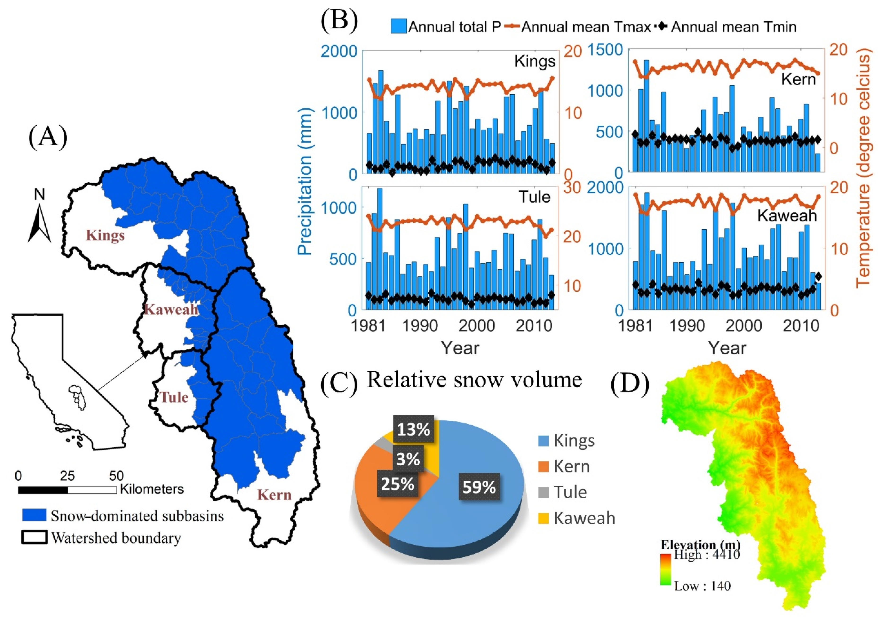
2. Study Area
3. Methods
3.1. Data
3.2. SWAT Model Implementation and Calibration
3.2.1. SWAT Model Implementation
3.2.2. SWAT Model Calibration
3.2.3. Evaluation of Calibration Scenarios
3.3. Evaluating the Impact of Parameter Equifinality on Model Predictions
4. Results
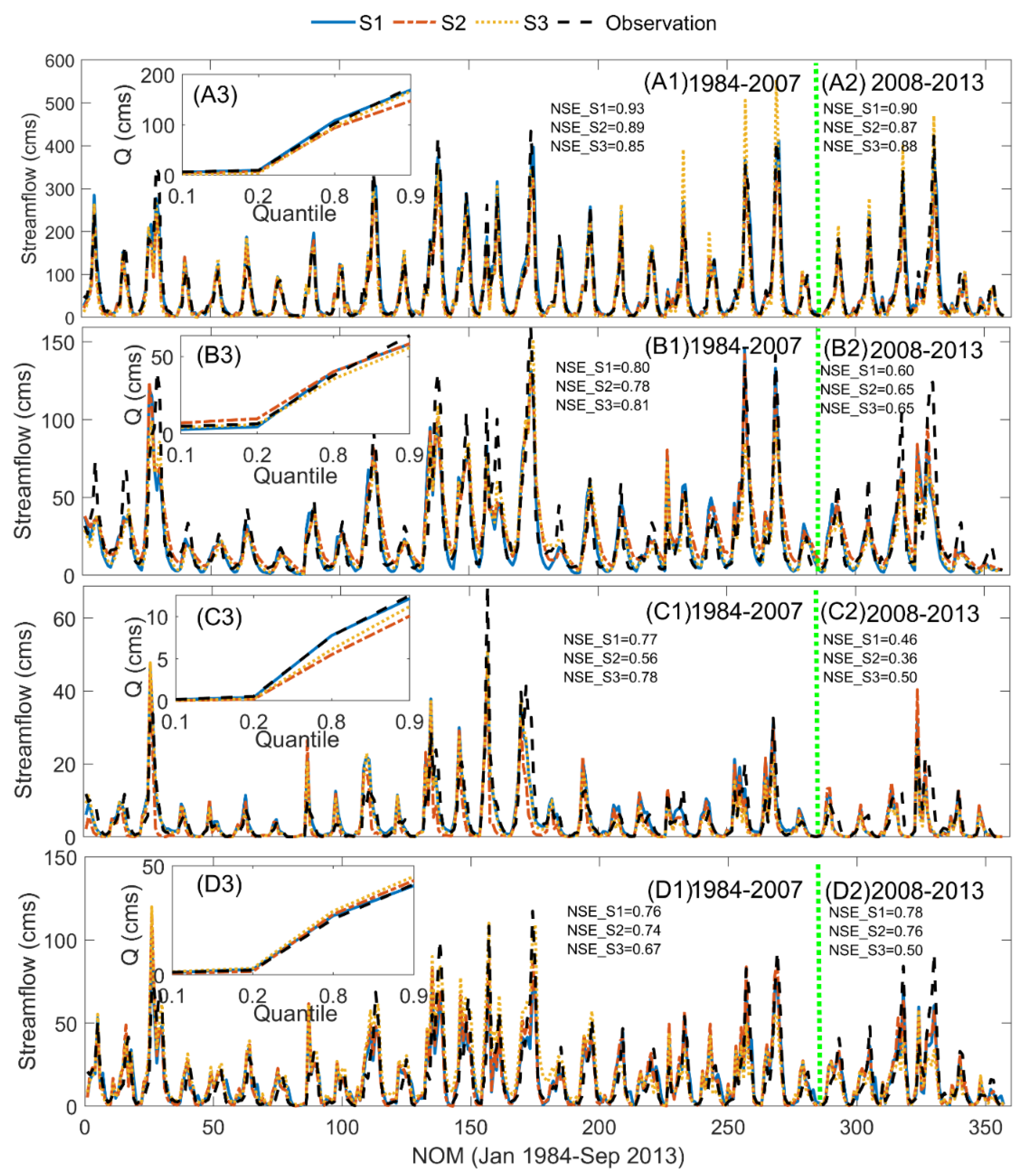
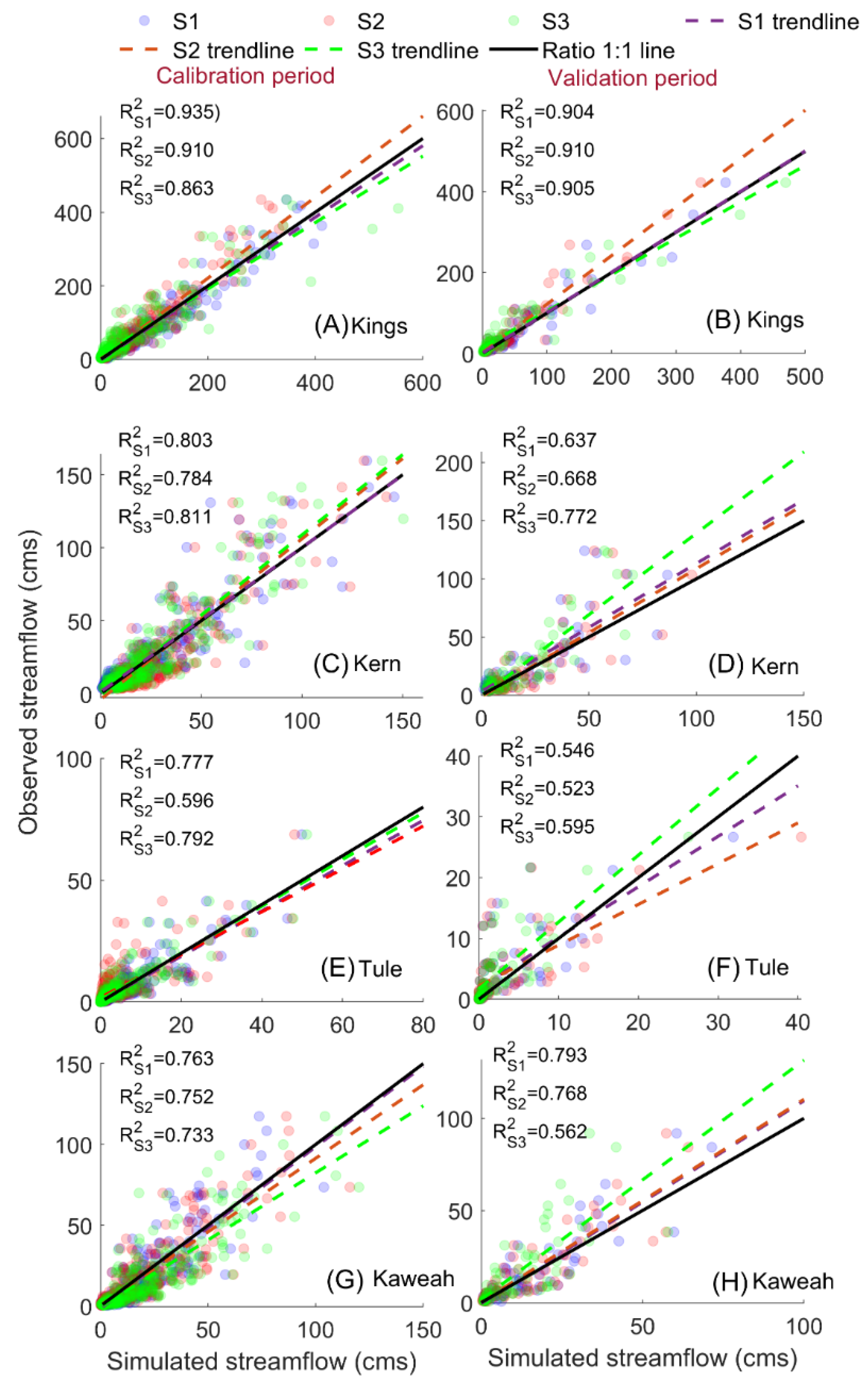
4.1. Impact of Three Model Calibration Scenarios on the Streamflow Predictions
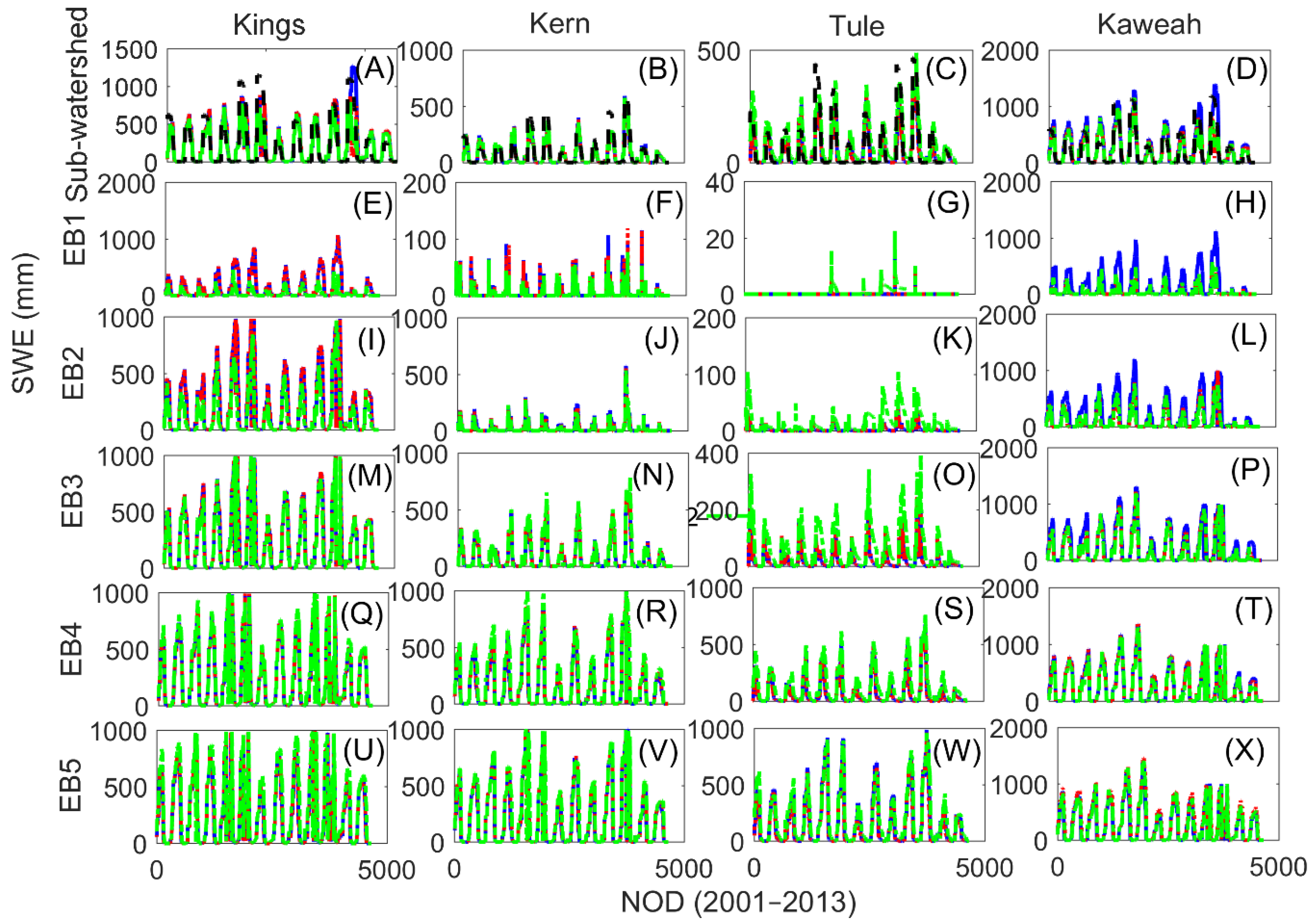
4.2. Impact of the Three Model Calibration Scenarios on the SWE Predictions
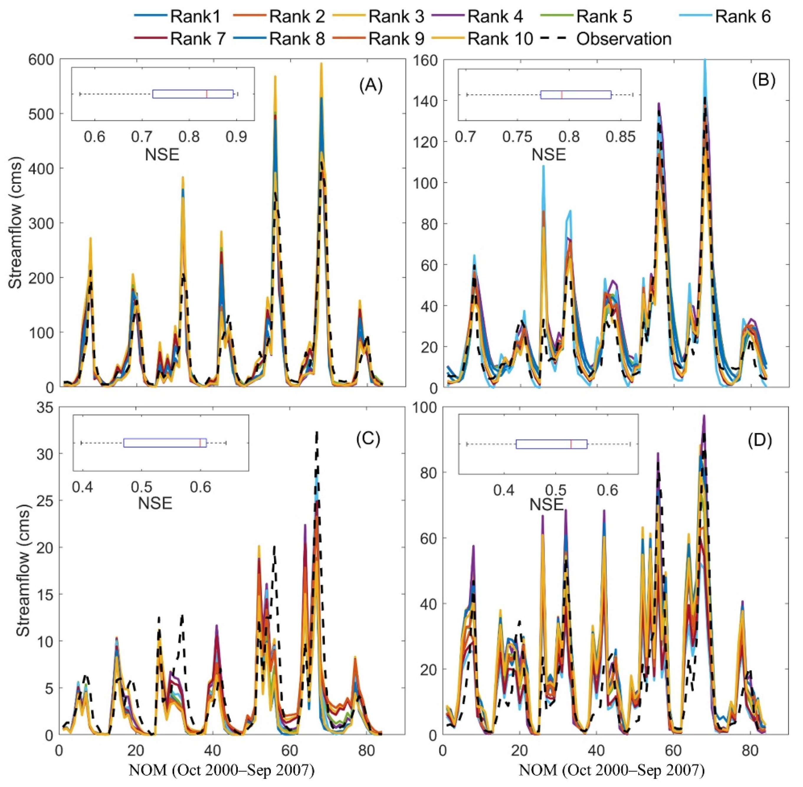
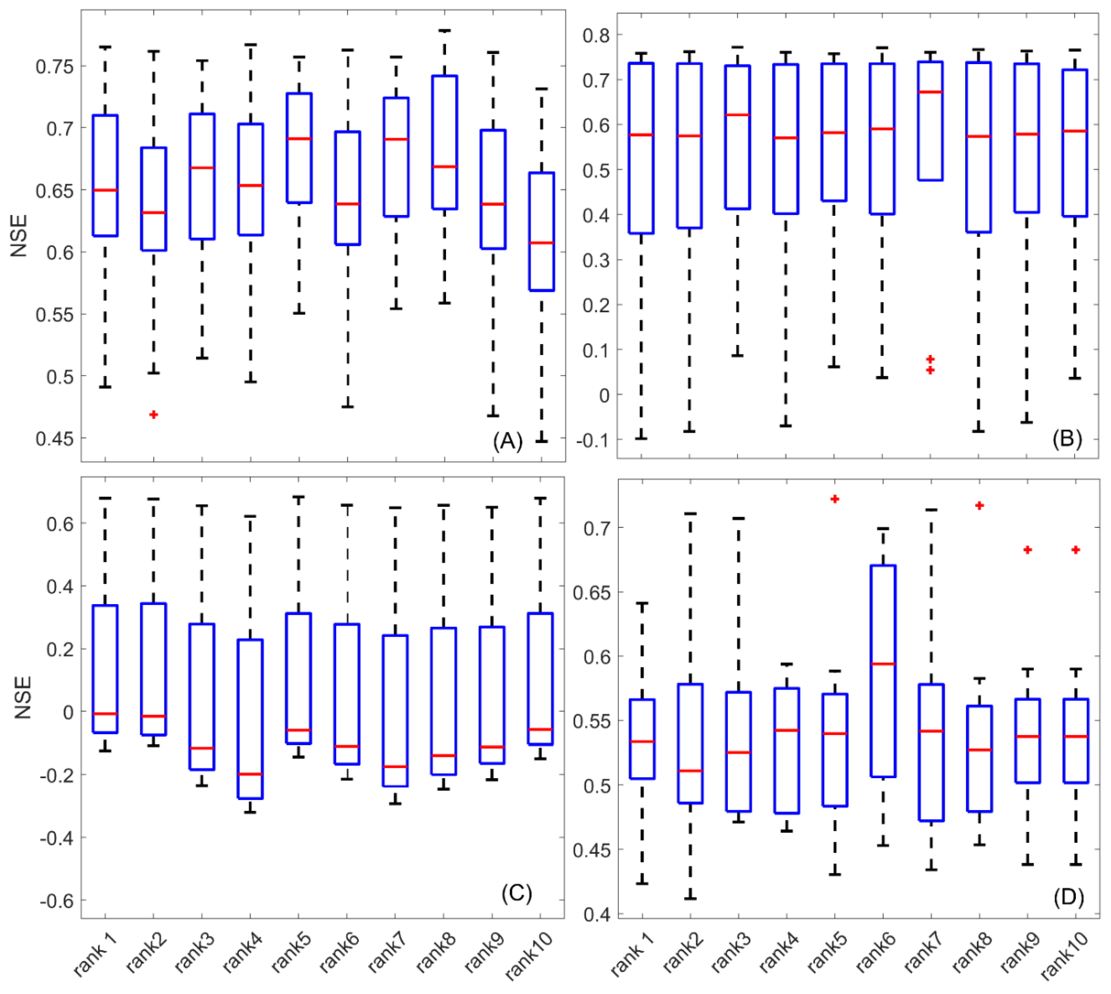
4.3. Influence of Parameter Equifinality on the Prediction Reliability
5. Discussions
5.1. Applying ParBal-Reconstructed SWE Data in the Calibration Process
5.2. The Role of Snow Parameters in SWAT Model Predictions
5.3. The Impact of Parameter Equifinality on the Model Prediction
6. Summary and Conclusions
- Although all three calibration strategies provide satisfactory streamflow predictions in general, slight differences exist among the three modeling scenarios, and the S3 calibration scenario does not always perform the best for streamflow prediction accuracy. In general, S2 performs slightly worse than the S1 scenario, which indicates that involving model parameter complexity might have a negative impact on the streamflow predictions if the model is calibrated only with a streamflow.
- The S3 calibration scenario shows its advantages for SWE predictions compared with S1 and S2. Even though, in some cases, the maximum NSE values of the sub-watersheds are not the highest after snow calibration, the variations are smaller. Therefore, the two-stage calibration strategy is recommended under the lumped calibration scheme for the upland watersheds, where snow plays a significant role.
- The S1 modeling scenario with default parameter values provides the best prediction for high flow conditions (related to floods), whereas no obvious differences exist among the three scenarios in simulating low flow conditions (droughts).
- All three scenarios work well for capturing large amounts of snow in the high elevations; however, the S3 scenario performs better than the other two scenarios in capturing small amounts of SWE in low elevations.
- The streamflow predictions are affected by the equifinality issue, and the changes of the NSE values vary between 0.2–0.3 for the ten parameter sets. Comparatively, the SWE prediction is also affected by the equifinality issue; however, the influence is slighter; the variation of the NSE is less than 0.1 for most cases.
- SWAT users are suggested to apply the appropriate number of calibration parameters and reference datasets for the goal (i.e., SWE and streamflow, in this study) that they are interested in. In most cases, there is no need to involve extra parameter complexity that is not related to the goal, and it might have a negative impact on the model predictions.
Author Contributions
Funding
Acknowledgments
Conflicts of Interest
Appendix A

| Kings Watershed | ||||||||||
| Parameter | 1 | 2 | 3 | 4 | 5 | 6 | 7 | 8 | 9 | 10 |
| V_SFTMP | 1.57 | 3.23 | 4.46 | 2.48 | 4.51 | 3.94 | 2.03 | 3.19 | 0.60 | 2.15 |
| V_SMTMP | 2.76 | 1.72 | 2.74 | 1.21 | 4.18 | 3.24 | 3.85 | 4.85 | 4.78 | 4.26 |
| V_SMFMX | 2.79 | 2.41 | 1.33 | 2.97 | 2.21 | 4.19 | 2.01 | 3.43 | 5.89 | 4.85 |
| V_SMFMN | 0.63 | 1.57 | 1.03 | 0.03 | 2.75 | 1.95 | 0.89 | 2.71 | 1.51 | 5.01 |
| V_TIMP | 0.97 | 0.82 | 0.96 | 0.82 | 0.86 | 0.90 | 0.85 | 0.89 | 0.81 | 0.89 |
| V_SNOCOVMX | 444.5 | 498.5 | 129.5 | 344.5 | 132.5 | 36.5 | 345.5 | 25.5 | 29.5 | 56.5 |
| V_SNO50COV | 0.22 | 0.03 | 0.71 | 0.19 | 0.36 | 0.68 | 0.34 | 0.67 | 0.93 | 0.59 |
| r_HRU_SLP | 0.21 | 0.82 | 0.32 | −0.41 | 0.51 | 0.53 | −0.31 | 0.74 | 0.47 | 0.70 |
| r_CN2 | 0.48 | −0.39 | 0.39 | 0.26 | 0.02 | −0.42 | 0.18 | −0.16 | −0.16 | 0.04 |
| V_ALPHA_BF | 0.92 | 0.98 | 0.95 | 0.05 | 0.68 | 0.21 | 0.79 | 0.02 | 0.76 | 0.94 |
| V_GW_DELAY | 97.5 | 437.5 | 320.5 | 478.5 | 26.5 | 259.5 | 81.5 | 54.5 | 330.5 | 486.5 |
| r_SOL_AWC | −0.36 | −0.42 | 0.08 | −0.12 | −0.34 | 0.39 | −0.30 | 0.29 | −0.36 | 0.33 |
| V_GWQMN | 4175 | 3575 | 3555 | 3065 | 4365 | 2715 | 1295 | 1145 | 4045 | 385 |
| V_RCHRG_DP | 0.20 | 0.68 | 0.82 | 0.57 | 0.65 | 0.63 | 0.61 | 0.48 | 0.68 | 0.28 |
| V_TLAPSE | −7.91 | −8.87 | −1.57 | −7.79 | −2.99 | −8.51 | −2.21 | −5.11 | −8.79 | −9.91 |
| V_PLAPSE | 16.50 | 88.70 | 58.10 | 48.5 | 17.30 | 44.5 | 98.30 | 95.90 | 5.3 | 39.5 |
| NSE | 0.886 | 0.866 | 0.864 | 0.839 | 0.833 | 0.831 | 0.828 | 0.826 | 0.817 | 0.812 |
| Kern Watershed | ||||||||||
| Parameter | 1 | 2 | 3 | 4 | 5 | 6 | 7 | 8 | 9 | 10 |
| V_SFTMP | 4.88 | 4.19 | 4.86 | 4.55 | 3.64 | 4.87 | 4.73 | 4.20 | 4.74 | 3.77 |
| V_SMTMP | 1.14 | 3.67 | 3.94 | 4.49 | 3.47 | 3.74 | 4.04 | 3.51 | 3.59 | 3.76 |
| V_SMFMX | 7.75 | 6.97 | 7.91 | 7.84 | 7.57 | 7.63 | 7.68 | 7.66 | 7.63 | 7.74 |
| V_SMFMN | 1.14 | 0.69 | 0.93 | 1.46 | 1.28 | 0.74 | 0.99 | 0.93 | 1.49 | 1.54 |
| V_TIMP | 0.92 | 0.95 | 0.93 | 0.91 | 0.92 | 0.90 | 0.95 | 0.95 | 0.91 | 0.91 |
| V_SNOCOVMX | 479.89 | 399.11 | 383.90 | 359.90 | 357.20 | 386.26 | 440.01 | 450.82 | 381.53 | 482.93 |
| V_SNO50COV | 0.45 | 0.45 | 0.39 | 0.45 | 0.40 | 0.46 | 0.33 | 0.45 | 0.29 | 0.41 |
| r_HRU_SLP | −0.83 | −0.69 | −0.74 | −0.82 | −0.80 | −0.84 | −0.78 | −0.71 | −0.77 | −0.81 |
| r_CN2 | −0.11 | −0.18 | −0.08 | −0.01 | −0.05 | −0.08 | −0.15 | −0.17 | −0.15 | 0.00 |
| V_ALPHA_BF | 0.06 | 0.05 | 0.05 | 0.05 | 0.05 | 0.15 | 0.09 | 0.05 | 0.08 | 0.05 |
| V_GW_DELAY | 168.98 | 254.04 | 313.07 | 278.35 | 319.57 | 245.79 | 145.98 | 118.20 | 222.36 | 241.89 |
| r_SOL_AWC | −0.01 | −0.11 | −0.18 | −0.11 | 0.05 | −0.10 | 0.06 | −0.14 | 0.04 | −0.08 |
| V_GWQMN | 3469 | 3710.12 | 4295.67 | 4673.77 | 3937.65 | 4948.14 | 4493.08 | 3974.45 | 3338.71 | 3994.53 |
| V_GW_REVAP | 0.10 | 0.10 | 0.08 | 0.09 | 0.12 | 0.08 | 0.10 | 0.11 | 0.08 | 0.08 |
| V_RCHRG_DP | 0.44 | 0.59 | 0.56 | 0.58 | 0.44 | 0.52 | 0.54 | 0.37 | 0.60 | 0.43 |
| V_TLAPSE | −6.54 | −6.52 | −8.28 | −6.37 | −7.59 | −7.42 | −7.30 | −6.86 | −6.74 | −7.76 |
| V_PLAPSE | 75.60 | 73.30 | 70.93 | 54.10 | 64.53 | 73.02 | 56.88 | 78.31 | 49.92 | 75.46 |
| NSE | 0.815 | 0.800 | 0.798 | 0.795 | 0.789 | 0.788 | 0.787 | 0.784 | 0.779 | 0.778 |
| Tule Watershed | ||||||||||
| Parameter | 1 | 2 | 3 | 4 | 5 | 6 | 7 | 8 | 9 | 10 |
| V_SFTMP | 4.52 | 3.91 | 4.37 | 4.36 | 4.23 | 4.28 | 3.64 | 3.77 | 3.80 | 4.06 |
| V_SMTMP | 1.98 | 1.85 | 1.21 | 3.67 | 3.11 | 2.90 | 3.70 | 1.15 | 2.98 | 3.39 |
| V_SMFMX | 5.09 | 6.30 | 5.33 | 4.27 | 5.15 | 5.40 | 2.70 | 5.70 | 6.39 | 4.44 |
| V_SMFMN | 5.69 | 5.04 | 4.72 | 5.51 | 4.40 | 5.22 | 3.00 | 4.68 | 4.49 | 6.38 |
| V_TIMP | 0.93 | 0.87 | 0.91 | 0.88 | 0.86 | 0.92 | 0.92 | 0.84 | 0.85 | 0.85 |
| V_SNOCOVMX | 336.35 | 354.82 | 417.06 | 342.85 | 391.42 | 368.16 | 375.00 | 408.17 | 448.87 | 340.46 |
| V_SNO50COV | 0.65 | 0.82 | 0.68 | 0.79 | 0.55 | 0.66 | 0.64 | 0.49 | 0.42 | 0.67 |
| r_HRU_SLP | −0.79 | −0.84 | −0.81 | −0.80 | −0.78 | −0.79 | −0.82 | −0.83 | −0.84 | −0.83 |
| r_CN2 | −0.49 | −0.33 | −0.39 | −0.48 | −0.43 | −0.48 | −0.48 | −0.46 | −0.48 | −0.24 |
| V_ALPHA_BF | 0.53 | 0.33 | 0.43 | 0.44 | 0.38 | 0.27 | 0.45 | 0.51 | 0.55 | 0.56 |
| V_GW_DELAY | 95.10 | 71.88 | 181.54 | 103 | 117.82 | 61.50 | 186.98 | 108.93 | 216.62 | 56.07 |
| r_SOL_AWC | 0.22 | 0.13 | 0.36 | 0.09 | 0.29 | 0.13 | 0.18 | 0.17 | 0.11 | 0.34 |
| V_GWQMN | 931.16 | 1431.35 | 261.26 | 288.06 | 1150 | 305.92 | 372.91 | 1918.15 | 792.72 | 1525.14 |
| V_GW_REVAP | 0.07 | 0.07 | 0.07 | 0.06 | 0.06 | 0.08 | 0.08 | 0.07 | 0.06 | 0.05 |
| V_RCHRG_DP | 0.07 | 0.11 | 0.03 | 0.27 | 0.079 | 0.27 | 0.04 | 0.13 | 0.002 | 0.14 |
| V_TLAPSE | −6.94 | −6.30 | −4.69 | −2.81 | −6.06 | −5 | −3.89 | −4.37 | −4.92 | −6.45 |
| V_PLAPSE | 27.32 | 32.91 | 29.75 | 27.02 | 18.75 | 23.06 | 15.52 | 28.17 | 19.35 | 17.35 |
| NSE | 0.808 | 0.785 | 0.774 | 0.773 | 0.771 | 0.759 | 0.758 | 0.754 | 0.749 | 0.747 |
| Kaweah Watershed | ||||||||||
| Parameter | 1 | 2 | 3 | 4 | 5 | 6 | 7 | 8 | 9 | 10 |
| V_SFTMP | 3.66 | 4.37 | 4.27642 | 3.52 | 3.46 | 2.74 | 4.12 | 4.70 | 3.23 | 3.45 |
| V_SMTMP | 2.26 | 2.45 | 0.85 | 1.07 | 0.89 | 0.97 | 1.02 | 1.61 | 1.12 | 2.35 |
| V_SMFMX | 3.81 | 4.82 | 3.01 | 3.87 | 5.27 | 4.66 | 3.18 | 2.05 | 1.95 | 5.61 |
| V_SMFMN | 0.70 | 1.93 | 0.22 | 0.79 | 0.46 | 0.50 | 1.09 | 1.10 | 1.08 | 0.11 |
| V_TIMP | 0.96 | 0.97 | 0.97 | 0.89 | 0.93 | 0.90 | 0.99 | 0.93 | 0.89 | 0.92 |
| V_SNOCOVMX | 330.56 | 498.60 | 483.98 | 419.35 | 259.75 | 267.05 | 272.67 | 323.25 | 392.94 | 378.33 |
| V_SNO50COV | 0.66 | 0.41 | 0.78 | 0.48 | 0.78 | 0.55 | 0.32 | 0.82 | 0.59 | 0.76 |
| r_HRU_SLP | −0.81 | −0.75 | −0.70 | −0.79 | −0.77 | −0.83 | −0.82 | −0.69 | −0.80 | −0.70 |
| r_CN2 | −0.34 | −0.47 | −0.19 | −0.22 | −0.27 | −0.48 | −0.36 | −0.26 | −0.28 | −0.30 |
| V_ALPHA_BF | 0.58 | 0.86 | 0.65 | 0.56 | 0.83 | 0.73 | 0.48 | 0.87 | 0.93 | 0.58 |
| V_GW_DELAY | 104.32 | 291.52 | 134.88 | 42.57 | 13.33 | 181.67 | 173.88 | 73.13 | 20.47 | 147.88 |
| r_SOL_AWC | −0.04 | 0.19 | −0.02 | −0.15 | −0.30 | −0.15 | −0.17 | 0.15 | 0.19 | −0.14 |
| V_GWQMN | 2655 | 2391.41 | 2561.47 | 2259.74 | 4174.36 | 3746.45 | 4103.04 | 4733.93 | 4212.76 | 2402.38 |
| V_GW_REVAP | 0.09 | 0.10 | 0.09 | 0.17 | 0.10 | 0.11 | 0.16 | 0.15 | 0.17 | 0.16 |
| V_RCHRG_DP | 0.40 | 0.58 | 0.58 | 0.47 | 0.42 | 0.42 | 0.36 | 0.44 | 0.22 | 0.33 |
| V_TLAPSE | −2.36 | −6.13 | −3.393 | −1.79 | −3.74 | −5.30 | −4.55 | −3.59 | −2.73 | −4.13 |
| V_PLAPSE | 55.90 | 6.06 | 37.41 | 38.16 | 15.05 | 32.42 | 14.80 | 31.92 | 5.18 | 23.30 |
| NSE | 0.697 | 0.672 | 0.657 | 0.655 | 0.648 | 0.645 | 0.645 | 0.625 | 0.621 | 0.619 |
References
- Dozier, J. Mountain hydrology, snow color, and the fourth paradigm. EOS Trans. Am. Geophys. Union 2011, 92, 373–374. [Google Scholar] [CrossRef]
- Bales, R.C.; Molotch, N.P.; Painter, T.H.; Dettinger, M.D.; Rice, R.; Dozier, J. Mountain hydrology of the western United States. Water Resour. Res. 2006, 42. [Google Scholar] [CrossRef]
- Biemans, H.; Siderius, C.; Lutz, A.; Nepal, S.; Ahmad, B.; Hassan, T.; Von Bloh, W.; Wijngaard, R.; Wester, P.; Shrestha, A. Importance of snow and glacier meltwater for agriculture on the Indo-Gangetic Plain. Nat. Sustain. 2019, 2, 594–601. [Google Scholar] [CrossRef]
- Mankin, J.S.; Viviroli, D.; Singh, D.; Hoekstra, A.Y.; Diffenbaugh, N.S. The potential for snow to supply human water demand in the present and future. Environ. Res. Lett. 2015, 10, 114016. [Google Scholar] [CrossRef]
- Simpkins, G. Snow-related water woes. Nat. Clim. Chang. 2018, 8, 945. [Google Scholar] [CrossRef]
- Gonzales-Inca, C.; Valkama, P.; Lill, J.-O.; Slotte, J.; Hietaharju, E.; Uusitalo, R. Spatial modeling of sediment transfer and identification of sediment sources during snowmelt in an agricultural watershed in boreal climate. Sci. Total Environ. 2018, 612, 303–312. [Google Scholar] [CrossRef]
- Liu, Z.; Herman, J.D.; Huang, G.; Kadir, T.; Dahlke, H. Identifying climate change impacts on surface water supply in the southern Central Valley, California. Sci. Total Environ. 2020, 143429. [Google Scholar] [CrossRef]
- Barnett, T.P.; Adam, J.C.; Lettenmaier, D.P. Potential impacts of a warming climate on water availability in snow-dominated regions. Nature 2005, 438, 303–309. [Google Scholar] [CrossRef]
- Clifton, C.F.; Day, K.T.; Luce, C.H.; Grant, G.E.; Safeeq, M.; Halofsky, J.E.; Staab, B.P. Effects of climate change on hydrology and water resources in the Blue Mountains, Oregon, USA. Clim. Serv. 2018, 10, 9–19. [Google Scholar] [CrossRef]
- Thackeray, C.W.; Derksen, C.; Fletcher, C.G.; Hall, A. Snow and Climate: Feedbacks, Drivers, and Indices of Change. Curr. Clim. Chang. Rep. 2019, 5, 322–333. [Google Scholar] [CrossRef]
- Coppola, E.; Raffaele, F.; Giorgi, F. Impact of climate change on snow melt driven runoff timing over the Alpine region. Clim. Dyn. 2018, 51, 1259–1273. [Google Scholar] [CrossRef]
- Schöner, W.; Koch, R.; Matulla, C.; Marty, C.; Tilg, A.M. Spatiotemporal patterns of snow depth within the Swiss-Austrian Alps for the past half century (1961 to 2012) and linkages to climate change. Int. J. Climatol. 2019, 39, 1589–1603. [Google Scholar] [CrossRef]
- Liu, Z.; Mehran, A.; Phillips, T.J.; Aghakouchak, A. Seasonal and regional biases in CMIP5 precipitation simulations. Clim. Res. 2014, 60, 35–50. [Google Scholar] [CrossRef]
- Dierauer, J.R.; Allen, D.M.; Whitfield, P.H. Snow drought risk and susceptibility in the western United States and southwestern Canada. Water Resour. Res. 2019, 55, 3076–3091. [Google Scholar] [CrossRef]
- Musselman, K.N.; Lehner, F.; Ikeda, K.; Clark, M.P.; Prein, A.F.; Liu, C.; Barlage, M.; Rasmussen, R. Projected increases and shifts in rain-on-snow flood risk over western North America. Nat. Clim. Chang. 2018, 8, 808–812. [Google Scholar] [CrossRef]
- Liu, Z.; Merwade, V. Accounting for model structure, parameter and input forcing uncertainty in flood inundation modeling using Bayesian model averaging. J. Hydrol. 2018, 565, 138–149. [Google Scholar] [CrossRef]
- Liu, Z.; Merwade, V. Separation and prioritization of uncertainty sources in a raster based flood inundation model using hierarchical Bayesian model averaging. J. Hydrol. 2019, 578, 124100. [Google Scholar] [CrossRef]
- Liu, Z.; Merwade, V.; Jafarzadegan, K. Investigating the role of model structure and surface roughness in generating flood inundation extents using one-and two-dimensional hydraulic models. J. Flood Risk Manag. 2019, 12, e12347. [Google Scholar] [CrossRef] [Green Version]
- Rajib, A.; Liu, Z.; Merwade, V.; Tavakoly, A.A.; Follum, M.L. Towards a large-scale locally relevant flood inundation modeling framework using SWAT and LISFLOOD-FP. J. Hydrol. 2020, 581, 124406. [Google Scholar] [CrossRef]
- Merwade, V.; Rajib, A.; Liu, Z. An integrated approach for flood inundation modeling on large scales. In Bridging Science and Policy Implication for Managing Climate Extremes; World Scientific Publication Company: Singapore, 2018; pp. 133–155. ISBN 978-981-3235-65-6. [Google Scholar] [CrossRef]
- Rajib, A.; Merwade, V.; Liu, Z. Large scale high resolution flood inundation mapping in near real-time. In Proceedings of the 40th Anniversary of the Association of State Flood Plain Managers National Conference, Gran Rapids, MI, USA, 19–24 June 2016; pp. 1–9. [Google Scholar]
- Dong, C.; Macdonald, G.M.; Willis, K.; Gillespie, T.W.; Okin, G.S.; Williams, A.P. Vegetation Responses to 2012–2016 Drought in Northern and Southern California. Geophys. Res. Lett. 2019, 46, 3810–3821. [Google Scholar] [CrossRef]
- Small, E.; Roesler, C.; Larson, K. Vegetation response to the 2012–2014 California drought from GPS and optical measurements. Remote Sens. 2018, 10, 630. [Google Scholar] [CrossRef] [Green Version]
- Mann, M.E.; Gleick, P.H. Climate change and California drought in the 21st century. Proc. Natl. Acad. Sci. USA 2015, 112, 3858–3859. [Google Scholar] [CrossRef] [PubMed] [Green Version]
- Shukla, S.; Safeeq, M.; Aghakouchak, A.; Guan, K.; Funk, C. Temperature impacts on the water year 2014 drought in California. Geophys. Res. Lett. 2015, 42, 4384–4393. [Google Scholar] [CrossRef] [Green Version]
- Stewart, I.T.; Cayan, D.R.; Dettinger, M.D. Changes in snowmelt runoff timing in western North America under abusiness as usual’climate change scenario. Clim. Chang. 2004, 62, 217–232. [Google Scholar] [CrossRef]
- Aurela, M.; Laurila, T.; Tuovinen, J.P. The timing of snow melt controls the annual CO2 balance in a subarctic fen. Geophys. Res. Lett. 2004, 31. [Google Scholar] [CrossRef]
- Lau, W.K.; Kim, M.-K.; Kim, K.-M.; Lee, W.-S. Enhanced surface warming and accelerated snow melt in the Himalayas and Tibetan Plateau induced by absorbing aerosols. Environ. Res. Lett. 2010, 5, 025204. [Google Scholar] [CrossRef]
- Kocis, T.N.; Dahlke, H.E. Availability of high-magnitude streamflow for groundwater banking in the Central Valley, California. Environ. Res. Lett. 2017, 12, 084009. [Google Scholar] [CrossRef]
- Najafi, M.; Moradkhani, H.; Jung, I. Assessing the uncertainties of hydrologic model selection in climate change impact studies. Hydrol. Process. 2011, 25, 2814–2826. [Google Scholar] [CrossRef]
- Mendoza, P.A.; Clark, M.P.; Mizukami, N.; Newman, A.J.; Barlage, M.; Gutmann, E.D.; Rasmussen, R.M.; Rajagopalan, B.; Brekke, L.D.; Arnold, J.R. Effects of hydrologic model choice and calibration on the portrayal of climate change impacts. J. Hydrometeorol. 2015, 16, 762–780. [Google Scholar] [CrossRef]
- Foster, L.M.; Bearup, L.A.; Molotch, N.P.; Brooks, P.D.; Maxwell, R.M. Energy budget increases reduce mean streamflow more than snow–rain transitions: Using integrated modeling to isolate climate change impacts on Rocky Mountain hydrology. Environ. Res. Lett. 2016, 11, 044015. [Google Scholar] [CrossRef]
- Mcnamara, J.P. Rain or snow: Hydrologic processes, observations, prediction, and research needs. Hydrol. Earth Syst. Sci. 2017, 21, 1–22. [Google Scholar]
- Wulf, H.; Bookhagen, B.; Scherler, D. Differentiating between rain, snow, and glacier contributions to river discharge in the western Himalaya using remote-sensing data and distributed hydrological modeling. Adv. Water Resour. 2016, 88, 152–169. [Google Scholar] [CrossRef] [Green Version]
- Qi, J.; Li, S.; Li, Q.; Xing, Z.; Bourque, C.P.-A.; Meng, F.-R. A new soil-temperature module for SWAT application in regions with seasonal snow cover. J. Hydrol. 2016, 538, 863–877. [Google Scholar] [CrossRef]
- Cibin, R.; Sudheer, K.; Chaubey, I. Sensitivity and identifiability of stream flow generation parameters of the SWAT model. Hydrol. Process. Int. J. 2010, 24, 1133–1148. [Google Scholar] [CrossRef]
- Thampi, S.G.; Raneesh, K.Y.; Surya, T. Influence of scale on SWAT model calibration for streamflow in a river basin in the humid tropics. Water Resour. Manag. 2010, 24, 4567–4578. [Google Scholar] [CrossRef]
- Arnold, J.G.; Moriasi, D.N.; Gassman, P.W.; Abbaspour, K.C.; White, M.J.; Srinivasan, R.; Santhi, C.; Harmel, R.; Van Griensven, A.; Van Liew, M.W. SWAT: Model use, calibration, and validation. Trans. ASABE 2012, 55, 1491–1508. [Google Scholar] [CrossRef]
- Her, Y.; Chaubey, I. Impact of the numbers of observations and calibration parameters on equifinality, model performance, and output and parameter uncertainty. Hydrol. Process. 2015, 29, 4220–4237. [Google Scholar] [CrossRef]
- Bekele, E.G.; Nicklow, J.W. Multi-objective automatic calibration of SWAT using NSGA-II. J. Hydrol. 2007, 341, 165–176. [Google Scholar] [CrossRef]
- Zhang, X.; Srinivasan, R.; Liew, M.V. On the use of multi-algorithm, genetically adaptive multi-objective method for multi-site calibration of the SWAT model. Hydrol. Process. Int. J. 2010, 24, 955–969. [Google Scholar] [CrossRef]
- Rajib, M.A.; Merwade, V.; Yu, Z. Multi-objective calibration of a hydrologic model using spatially distributed remotely sensed/in-situ soil moisture. J. Hydrol. 2016, 536, 192–207. [Google Scholar] [CrossRef] [Green Version]
- Yin, J.; Pham, H.V.; Tsai, F.T.-C. Multiobjective Spatial Pumping Optimization for Groundwater Management in a Multiaquifer System. J. Water Resour. Plan. Manag. 2020, 146, 04020013. [Google Scholar] [CrossRef]
- Schneider, D.; Molotch, N.P. Real-time estimation of snow water equivalent in the U pper C olorado R iver B asin using MODIS-based SWE Reconstructions and SNOTEL data. Water Resour. Res. 2016, 52, 7892–7910. [Google Scholar] [CrossRef]
- Troin, M.; Caya, D. Evaluating the SWAT’s snow hydrology over a Northern Quebec watershed. Hydrol. Process. 2014, 28, 1858–1873. [Google Scholar] [CrossRef]
- Dozier, J.; Bair, E.H.; Davis, R.E. Estimating the spatial distribution of snow water equivalent in the world’s mountains. Wiley Interdiscip. Rev. Water 2016, 3, 461–474. [Google Scholar] [CrossRef]
- Lettenmaier, D.P.; Alsdorf, D.; Dozier, J.; Huffman, G.J.; Pan, M.; Wood, E.F. Inroads of remote sensing into hydrologic science during the WRR era. Water Resour. Res. 2015, 51, 7309–7342. [Google Scholar] [CrossRef]
- De Gregorio, L.; Günther, D.; Callegari, M.; Strasser, U.; Zebisch, M.; Bruzzone, L.; Notarnicola, C. Improving SWE Estimation by Fusion of Snow Models with Topographic and Remotely Sensed Data. Remote Sens. 2019, 11, 2033. [Google Scholar] [CrossRef] [Green Version]
- Tedesco, M.; Narvekar, P.S. Assessment of the NASA AMSR-E SWE product. IEEE J. Sel. Top. Appl. Earth Obs. Remote Sens. 2010, 3, 141–159. [Google Scholar] [CrossRef]
- Molotch, N.P.; Painter, T.H.; Bales, R.C.; Dozier, J. Incorporating remotely-sensed snow albedo into a spatially-distributed snowmelt model. Geophys. Res. Lett. 2004, 31. [Google Scholar] [CrossRef] [Green Version]
- Rice, R.; Bales, R.C.; Painter, T.H.; Dozier, J. Snow water equivalent along elevation gradients in the Merced and Tuolumne River basins of the Sierra Nevada. Water Resour. Res. 2011, 47. [Google Scholar] [CrossRef]
- Girotto, M.; Margulis, S.A.; Durand, M. Probabilistic SWE reanalysis as a generalization of deterministic SWE reconstruction techniques. Hydrol. Process. 2014, 28, 3875–3895. [Google Scholar] [CrossRef]
- Walton, D.B.; Hall, A.; Berg, N.; Schwartz, M.; SUN, F. Incorporating snow albedo feedback into downscaled temperature and snow cover projections for California’s Sierra Nevada. J. Clim. 2017, 30, 1417–1438. [Google Scholar] [CrossRef]
- Marston, L.; Konar, M. Drought impacts to water footprints and virtual water transfers of the Central Valley of California. Water Resour. Res. 2017, 53, 5756–5773. [Google Scholar] [CrossRef]
- Faunt, C.C.; Sneed, M.; Traum, J.; Brandt, J.T. Water availability and land subsidence in the Central Valley, California, USA. Hydrogeol. J. 2016, 24, 675–684. [Google Scholar] [CrossRef] [Green Version]
- Lee, J.; De Gryze, S.; Six, J. Effect of climate change on field crop production in California’s Central Valley. Clim. Chang. 2011, 109, 335–353. [Google Scholar] [CrossRef]
- Margulis, S.A.; Cortés, G.; Girotto, M.; Durand, M. A Landsat-era Sierra Nevada snow reanalysis (1985–2015). J. Hydrometeorol. 2016, 17, 1203–1221. [Google Scholar] [CrossRef]
- Bair, E.H.; Rittger, K.; Skiles, S.M.; Dozier, J. An examination of snow albedo estimates from MODIS and their impact on snow water equivalent reconstruction. Water Resour. Res. 2019. [Google Scholar] [CrossRef]
- Rouholahnejad, E.; Abbaspour, K.C.; Vejdani, M.; Srinivasan, R.; Schulin, R.; Lehmann, A. A parallelization framework for calibration of hydrological models. Environ. Model. Softw. 2012, 31, 28–36. [Google Scholar] [CrossRef]
- Kumar, N.; Singh, S.K.; Srivastava, P.K.; Narsimlu, B. SWAT Model calibration and uncertainty analysis for streamflow prediction of the Tons River Basin, India, using Sequential Uncertainty Fitting (SUFI-2) algorithm. Model. Earth Syst. Environ. 2017, 3, 30. [Google Scholar] [CrossRef]
- Kadir, T.H.; Huang, G. Estimates of Natural and Unimpaired Flows for the Central Valley of California: Water Years 1922–2014; Report of California Department of Water Resources: Sacramento, CA, USA, 2016.
- Pradhanang, S.M.; Anandhi, A.; Mukundan, R.; Zion, M.S.; Pierson, D.C.; Schneiderman, E.M.; Matonse, A.; Frei, A. Application of SWAT model to assess snowpack development and streamflow in the Cannonsville watershed, New York, USA. Hydrol. Process. 2011, 25, 3268–3277. [Google Scholar] [CrossRef]
- Arnold, J.G.K.; Kiniry, J.R.; Srinivasan, R.; Williams, J.R.; Haney, E.B.; Neitsch, S.L. Soil & Water Assessment Tool Input/Output Documentation. Version 2012. Available online: https://swat.tamu.edu/media/69296/swat-io-documentation-2012.pdf (accessed on 13 November 2020).
- White, K.L.; Chaubey, I. Sensitivity analysis, calibration, and validations for a multisite and multivariable SWAT model 1. JAWRA J. Am. Water Resour. Assoc. 2005, 41, 1077–1089. [Google Scholar] [CrossRef]
- Abbaspour, K.C.; Rouholahnejad, E.; Vaghefi, S.; Srinivasan, R.; Yang, H.; Kløve, B. A continental-scale hydrology and water quality model for Europe: Calibration and uncertainty of a high-resolution large-scale SWAT model. J. Hydrol. 2015, 524, 733–752. [Google Scholar] [CrossRef] [Green Version]
- Xiao, M.; Koppa, A.; Mekonnen, Z.; Pagán, B.R.; Zhan, S.; CAO, Q.; Aierken, A.; Lee, H.; Lettenmaier, D.P. How much groundwater did California’s Central Valley lose during the 2012–2016 drought? Geophys. Res. Lett. 2017, 44, 4872–4879. [Google Scholar] [CrossRef]
- Griffin, D.; Anchukaitis, K.J. How unusual is the 2012–2014 California drought? Geophys. Res. Lett. 2014, 41, 9017–9023. [Google Scholar] [CrossRef] [Green Version]
- Beven, K. A manifesto for the equifinality thesis. J. Hydrol. 2006, 320, 18–36. [Google Scholar] [CrossRef] [Green Version]
- Beven, K.; Binley, A. The future of distributed models: Model calibration and uncertainty prediction. Hydrol. Process. 1992, 6, 279–298. [Google Scholar] [CrossRef]
- Ahl, R.S.; Woods, S.W.; Zuuring, H.R. Hydrologic calibration and validation of swat in a snow-dominated rocky mountain watershed, montana, USA 1. JAWRA J. Am. Water Resour. Assoc. 2008, 44, 1411–1430. [Google Scholar] [CrossRef]
- Wang, X.; Melesse, A. Evaluation of the SWAT model’s snowmelt hydrology in a northwestern Minnesota watershed. Trans. ASAE 2005, 48, 1359–1376. [Google Scholar] [CrossRef]
- Grusson, Y.; Sun, X.; Gascoin, S.; Sauvage, S.; Raghavan, S.; Anctil, F.; Sáchez-Pérez, J.-M. Assessing the capability of the SWAT model to simulate snow, snow melt and streamflow dynamics over an alpine watershed. J. Hydrol. 2015, 531, 574–588. [Google Scholar] [CrossRef]
- Stehr, A.; Debels, P.; Arumi, J.L.; Romero, F.; Alcayaga, H. Combining the Soil and Water Assessment Tool (SWAT) and MODIS imagery to estimate monthly flows in a data-scarce Chilean Andean basin. Hydrol. Sci. J. 2009, 54, 1053–1067. [Google Scholar] [CrossRef]
- Immerzeel, W.; Droogers, P. Calibration of a distributed hydrological model based on satellite evapotranspiration. J. Hydrol. 2008, 349, 411–424. [Google Scholar] [CrossRef]
- Tuo, Y.; Marcolini, G.; Disse, M.; Chiogna, G. Calibration of snow parameters in SWAT: Comparison of three approaches in the Upper Adige River basin (Italy). Hydrol. Sci. J. 2018, 63, 657–678. [Google Scholar] [CrossRef]
- Zhang, X.; Srinivasan, R.; Debele, B.; Hao, F. Runoff simulation of the headwaters of the yellow river using The SWAT model with three snowmelt algorithms 1. JAWRA J. Am. Water Resour. Assoc. 2008, 44, 48–61. [Google Scholar] [CrossRef]
- Fu, C.; James, A.L.; Yao, H. Investigations of uncertainty in SWAT hydrologic simulations: A case study of a Canadian Shield catchment. Hydrol. Process. 2015, 29, 4000–4017. [Google Scholar] [CrossRef]
- Yin, J.; Tsai, F.T.-C. Saltwater scavenging optimization under surrogate uncertainty for a multi-aquifer system. J. Hydrol. 2018, 565, 698–710. [Google Scholar] [CrossRef]
- Yin, J.; Tsai, F.T.-C. Bayesian set pair analysis and machine learning based ensemble surrogates for optimal multi-aquifer system remediation design. J. Hydrol. 2020, 580, 124280. [Google Scholar] [CrossRef]


| Parameter | Description | Initial Range | Kings | Kern | Tule | Kaweah | |
|---|---|---|---|---|---|---|---|
| Snow Parameters | V_SFTMP | Snowfall temperature (°C) | 0–5 | 4 | 4.8 | 4.58 | 4 |
| V_SMTMP | Snowmelt base temperature (°C) | 0–5 | 5 | 5 | 5 | 4.5 | |
| V_SMFMX | Melt factor for snow on June 21 (mm H2O/°C-day) | 0–10 | 5 | 8 | 4.59 | 5 | |
| V_SMFMN | Melt factor for snow on December 21 (mm H2O/°C-day) | 0–10 | 3 | 0.1 | 0.62 | 4 | |
| V_TIMP | Snow pack temperature lag factor | 0.8–1 | 0.88 | 0.9 | 0.86 | 0.8 | |
| V_SNOCOVMX | Minimum snow water content that corresponds to 100% snow cover, SNO100 (mm H2O) | 0–500 | 400 | 320 | 360.79 | 490 | |
| V_SNO50COV | Fraction of snow volume represented by SNOCOVMX that corresponds to 50% snow cover | 0.01–0.99 | 0.4 | 0.1 | 0.66 | 0.03 | |
| Watershed Parameters | r_HRU_SLP | Average slope steepness | −0.84–0.84 | 0.21 | −0.83 | −0.79 | −0.81 |
| r_CN2 | SCS curve number | −0.5–0.5 | 0.48 | −0.11 | −0.49 | −0.34 | |
| V_ALPHA_BF | Baseflow alpha factor (days) | 0–0.99 | 0.92 | 0.06 | 0.53 | 0.58 | |
| V_GW_DELAY | Groundwater Delay (days) | 0–500 | 97.5 | 169 | 95.1 | 104.32 | |
| r_SOL_AWC | Available water capacity of the soil layer (mm H2O/mm soil) | −0.5–0.5 | −0.36 | −0.013 | 0.22 | −0.044 | |
| V_GWQMN | shallow aquifer required for return flow to occur (mm) | 0–5000 | 4175 | 3469 | 931.16 | 2654.74 | |
| V_GW_REVAP | Groudwater “revap” coefficient | 0.02–0.2 | 0.18 | 0.096 | 0.073 | 0.085 | |
| V_RCHRG_DP | Deep aquifer percolation factor | 0–0.9 | 0.2 | 0.44 | 0.069 | 0.4 | |
| Elevation Lapse rate Parameters | V_TLAPSE | Temperature lapse rate (°C/km) | −10–0 | −7 | −8.5 | −9.12 | −7 |
| V_PLAPSE | Precipitation lapse rate (mm H2O/km) | 0–100 | 62.61 | 33.04 | 27.01 | 99.16 | |
| Description | Default Value in SWAT-CUP | |
|---|---|---|
| V_SFTMP | Snowfall temperature (°C) | 1.0 |
| V_SMTMP | Snowmelt base temperature (°C) | 0.5 |
| V_SMFMX | Melt factor for snow on 21 June (mm H2O/°C-day) | 4.5 |
| V_SMFMN | Melt factor for snow on 21 December (mm H2O/°C-day) | 4.5 |
| V_TIMP | Snow pack temperature lag factor | 1.0 |
| V_SNOCOVMX | Minimum snow water content that corresponds to 100% snow cover, SNO100 (mm H2O) | 1.0 |
| V_SNO50COV | Fraction of snow volume represented by SNOCOVMX that corresponds to 50% snow cover | 0.50 |
| Scenarios | S1 | S2 | S3 | |
|---|---|---|---|---|
| Streamflow calibration | Include? | YES | YES | YES |
| Period | 1981–2007 | 1981–2007 | 1981–2000 | |
| Reference data | Outlet streamflow | Outlet streamflow | Outlet streamflow | |
| Snow water equivalent calibration | Include? | No (with default snow parameter values applied) | Yes (calibration of snow parameters) | Yes (calibration of snow parameters) |
| Period | N/A | 1981–2007 | 2001–2007 | |
| Reference data | N/A | Outlet streamflow | Sub-watershed SWE | |
| Validation | Include? | YES | YES | YES |
| Period | 2008–2013 | 2008–2013 | 2008–2013 | |
| Validation objectives | Outlet Streamflow and sub-watershed SWE | Outlet Streamflow and sub-watershed SWE | Outlet Streamflow and sub-watershed SWE | |
| NSE | S1 | S2 | S3 |
|---|---|---|---|
| Kings | 0.5708 | 0.5300 | 0.6488 |
| Kern | 0.6900 | 0.6799 | 0.7204 |
| Tule | 0.6729 | 0.6554 | 0.6896 |
| Kaweah | 0.6932 | 0.6590 | 0.6478 |
Publisher’s Note: MDPI stays neutral with regard to jurisdictional claims in published maps and institutional affiliations. |
© 2020 by the authors. Licensee MDPI, Basel, Switzerland. This article is an open access article distributed under the terms and conditions of the Creative Commons Attribution (CC BY) license (http://creativecommons.org/licenses/by/4.0/).
Share and Cite
Liu, Z.; Yin, J.; E. Dahlke, H. Enhancing Soil and Water Assessment Tool Snow Prediction Reliability with Remote-Sensing-Based Snow Water Equivalent Reconstruction Product for Upland Watersheds in a Multi-Objective Calibration Process. Water 2020, 12, 3190. https://doi.org/10.3390/w12113190
Liu Z, Yin J, E. Dahlke H. Enhancing Soil and Water Assessment Tool Snow Prediction Reliability with Remote-Sensing-Based Snow Water Equivalent Reconstruction Product for Upland Watersheds in a Multi-Objective Calibration Process. Water. 2020; 12(11):3190. https://doi.org/10.3390/w12113190
Chicago/Turabian StyleLiu, Zhu, Jina Yin, and Helen E. Dahlke. 2020. "Enhancing Soil and Water Assessment Tool Snow Prediction Reliability with Remote-Sensing-Based Snow Water Equivalent Reconstruction Product for Upland Watersheds in a Multi-Objective Calibration Process" Water 12, no. 11: 3190. https://doi.org/10.3390/w12113190