Modeling River Runoff Temporal Behavior through a Hybrid Causal–Hydrological (HCH) Method
by
 , , , and
Santiago Zazo
1 ,
,
José-Luis Molina
1,* ,
,
Verónica Ruiz-Ortiz
2 ,
,
Mercedes Vélez-Nicolás
3 and
and
Santiago García-López
3 1
IGA Research Group, Higher Polytechnic School of Ávila, University of Salamanca, Av. de los Hornos Caleros, 50, 05003 Ávila, Spain
2
Department of Industrial Engineering and Civil Engineering, University of Cadiz, Campus Bay of Algeciras, Avda. Ramon Puyol s/n, 11202 Algeciras, Spain
3
Department of Earth Sciences, University of Cadiz, Campus Rio San Pedro, s/n, 11510 Puerto Real, Spain
*
Author to whom correspondence should be addressed.
Water 2020, 12(11), 3137; https://doi.org/10.3390/w12113137
Submission received: 17 September 2020
/
Revised: 4 November 2020
/
Accepted: 6 November 2020
/
Published: 9 November 2020
(This article belongs to the Special Issue Stochastic Modeling in Hydrology)
Abstract
:The uncertainty in traditional hydrological modeling is a challenge that has not yet been overcome. This research aimed to provide a new method called the hybrid causal–hydrological (HCH) method, which consists of the combination of traditional rainfall–runoff models with novel hydrological approaches based on artificial intelligence, called Bayesian causal modeling (BCM). This was implemented by building nine causal models for three sub-basins of the Barbate River Basin (SW Spain). The models were populated by gauging (observing) short runoff series and from long and short hydrological runoff series obtained from the Témez rainfall–runoff model (T-RRM). To enrich the data, all series were synthetically replicated using an ARMA model. Regarding the results, on the one hand differences in the dependence intensities between the long and short series were displayed in the dependence mitigation graphs (DMGs), which were attributable to the insufficient amount of data available from the hydrological records and to climate change processes. The similarities in the temporal dependence propagation (basin memory) and in the symmetry of DMGs validate the reliability of the hybrid methodology, as well as the results generated in this study. Consequently, water planning and management can be substantially improved with this approach.
1. Introduction
Currently, extreme events such as heavy rainfall, droughts, and floods are becoming more common and less exceptional [1,2,3,4,5], even within a particular territory [6,7], resulting in growing variability in certain hydrological processes [8,9], in addition to pressure on, and uncertainty regarding, water resources [10,11,12], which is especially noticeable using runoffs series [13]. In this sense, the frequency of droughts in Southern Europe is increasing significantly [14,15]. This is making it necessary to improve the knowledge on the temporal behavior of rivers [16,17,18], as not all the reasons that explain this increasing variability are new [16,18].
As such, there is a strong need to develop new analytical approaches capable of capturing the induced and widespread effects that these new hydrological phenomena are causing on water resource availability [19]. This is essential not only for planning and development of effective water resource management strategies [18], but also in terms of optimal dimensioning of hydraulic infrastructure, such as reservoirs [13,20].
The temporal behavior of rivers has traditionally received special attention from the scientific and engineering communities [16,20,21,22]. This topic has been developed through previous studies and approaches that are currently the benchmarks and through persistence, and is strongly related to the measurement of the long-term memory of time series using the Hurst coefficient [23], as well as storage and drought statistics [24]. This issue has mainly been addressed by models of: (1) the interactions between multiple physical factors, such as meteorological, geological, and hydrogeological factors [13]; and (2) the analysis of hydrological records [24]. Furthermore, it should firstly be noted that any model is an abstraction of reality [25], which is only partially known, and secondly, as is well-known, the scarcity of data has been a constant issue in hydrological research [26].
This has led to diverse points of view [22] on how to address these issues, which are essentially classified into two main approaches, deterministic and stochastic [27,28], as was detailed by Molina et al. [16]. Moreover, the growing global demand for water resources [29,30], negative scientific predictions of their availability due to climate change [31,32], and the partial knowledge of the underlying relationships in complex natural systems such as water systems [33,34,35,36] give this research special relevance.
Deterministic models, which are often complex, are characterized by (1) being accurate, (2) needing large amounts of data and even inputs from other models, (3) and by the data processing being time consuming and frequently based on a unique time series [16]. The above advantages allow a better understanding of the modeling process through the abstraction (i.e., simplification) of complex simulated natural phenomena [16]. This is especially useful in the case of controlled and gauged river basins that are barely affected by climate change [27]. Moreover, this general method is currently applied using software such as HEC-HMS [37] (which is widely accepted in the field of hydrological engineering [16]) by most water administrations [38]. However, the main weakness of these models is their limited capacity for analysis of certain relevant aspects, such as the temporal dependence or persistence of the basin´s memory [16,27], in addition to not being viable for basins with limited data [39].
In recent decades, stochastic-model-based approaches have emerged in the development of hydrological models as a result of advances in computer science [16,20,22,36,40]. These models are fundamentally different from the previous ones in how they deal with the uncertainty inherent in any hydrological process [27,41]. This distinctive feature makes them suitable for hydrological modeling [41]. Some relevant examples are autoregressive moving average (ARMA) and autoregressive integrated moving average (ARIMA) models, multivariate adaptive regression splines (MARS), and causal reasoning (CR). The theoretical backgrounds of all these approaches were covered in depth by Molina et al. [16,20].
In this sense, CR, as an artificial intelligence (AI) technique, is a powerful stochastic approach and is especially relevant to this research for the following reasons: (1) it uses raw data directly [42]; (2) it does not require “a priori” knowledge of the process [43]; (3) it handles a large amount of information from dynamic and non-linear systems [36]; (4) it is able to define sophisticated relationships in complex natural systems [44]; (5) it is a powerful tool for discovering causal structures in raw statistical data [45].
Additionally, as shown by the studies by Molina et al. [20] and Zazo [22], the potential for using causality to deal with temporal river behavior has recently begun to be explored using CR. This involves coupling traditional and novel methodologies through an ARMA model and Bayesian causal modeling (BCM). This has given rise to an active research area focused on increasing the knowledge of water resources and based on extracting the hidden logical time dependency structure that inherently underlies hydrological series. A comprehensive and in-depth theoretical and mathematical background and the main hydrological contributions to this research area are covered in [13,17,18,28].
The sustainability of a hydrological system as assessed through the characterization of basin memory is very relevant, especially in the short term. Consequently, this research work aims to capture that temporal signature through a hybrid causal framework, which combines the advantages of deterministic and stochastic models. This is mainly highlighted through the relationship between an input signal (rainfall) and an output signal (runoff).
Additionally, this work aims to overcome the lack of suitable and available hydrological data for CR analysis, as causal models need to be populated by as much information as possible to be representative [16]. This scarcity is largely due to several reservoirs having been built in the study basin (Almodovar, Celemín, and Barbate reservoirs) at the end of the 20th century in order to solve the problems related to recurrent droughts, floods, and water availability in this study zone.
In order to solve these challenges, a hybrid framework called the hybrid causal–hydrological (HCH) approach is developed in this study. This is done by hybridizing a BCM (stochastic platform) with a rainfall–runoff model (RRM) (deterministic module), which is the data source for the BCM platform.
Here, the RRM is the Témez RRM model (henceforth referred as T-RRM) [46,47,48]. This is an aggregate and semi-distributed model of parameters that is suitable for homogeneous basins with a reduced amount of data. The T-RRM model is well-established in hydrological engineering, particularly in Spain [15,49,50,51,52,53], and is supported here by EvalHid software [54]. The T-RRM can provide reliable and long-term natural regime runoff time series and is used here to generate synthetic series using a parsimonious and unconditioned ARMA model (first stochastic approach). Then, these equiprobable time series are used for causal reasoning (second stochastic series) and the results are analyzed in depth.
After this introductory section, this manuscript is organized as follows. A case study, dataset description, and the applied methodology are discussed in Section 2. Section 3 provides the main experimental results from the research. In Section 4, the results are discussed in detail. Lastly, Section 4 is devoted to the general conclusions drawn from the study.
2. Materials and Methods
2.1. Case Study
The Barbate River Basin is located in the province of Cadiz, southern Spain, near the Strait of Gibraltar. It covers an approximate area of 1330 km2, which includes a significant extension of Los Alcornocales Natural Park and a small sector at the SW of Breña and Marismas in the Barbate Natural Park. The basin has a smooth orography, with more than the 70% of its area ranging between 0 and 100 m; however, in its northeast sector, there are mountainous reliefs that reach 1090 m above sea level (m.a.s.l.; Figure 1a–c) [55].
The Köppen–Geiger classification describes the climate of this area as temperate, with hot, dry summers [56,57]. The basin is characterized by a Mediterranean climate with a strong oceanic influence, which is bolstered by its orography, in addition to a marked seasonal rainfall regime, with average annual values of 835 mm [55]. Additionally, the general rainfall pattern is characterized by strong interannual irregularity, with values ranging between 365 (dry years) and 1606 mm/year (wet years). The precipitation is mainly concentrated in autumn and winter months, with practically no precipitation in the summer period. The average annual temperature is 18 °C [55], with milder values in mountainous areas. In this sense, it should be noted that the study area is repeatedly affected by intense and persistent warm–dry wind periods, commonly known as Levante winds, which can last for 7 consecutive days, with an average velocity of 50 km/h and maximum velocities of up to 100 km/h [58,59]. This wind plays an important role in evaporation processes [55].
Geologically, the basin comprises a wide variety of materials. The oldest ones are Triassic Keuper facies (pre-orogenic), which are composed of multicolored gypsum-rich clays, sands, and limestones [60]. On these, tecto-sedimentary materials such as cemented siliceous sandstones and clays are overlaid, corresponding to turbiditic deposits [61]. Post-orogenic materials were subsequently deposited, filling the tertiary basins with sediments that were deposited in marine and coastal environments during the Upper Miocene and Pliocene (marls, biocalcarenites, and sands). Lastly, continental materials from the Quaternary age were deposited, with these being associated with recent sedimentary processes, aeolian and beach sands, alluvial material linked to river dynamics, and slope deposits [55].
In hydrogeological terms, two systems of a certain significance are located in the study area, named the Benalup aquifer (groundwater body GWB 062.014, of 33 km2) and the Barbate aquifer (GWB 062.013, of 93 km2). Both systems, which are constituted by biocalcarenites and sands, are characterized by an intergranular porosity that is locally increased by dissolution processes [62].
Regarding hydrological aspects, the main water course in the zone is the Barbate river, which is regulated by the Barbate dam (storage capacity of 228 Hm3) and its tributaries, the Álamo, Celemín, and Almodóvar rivers. The latter two are also regulated, in this case by the Celemín (45 Hm3) and Almodóvar (5.7 Hm3) dams, respectively (Figure 1c). The water resources for the Celemín and Barbate reservoirs are jointly used to irrigate an area measuring 122.3 Km2, whereas the Almodóvar reservoir is exploited for both irrigation (3.63 Km2) and for supply of the municipality of Tarifa. Finally, the basin’s water resources were estimated to be 247 Hm3/year for the period 1999–2016 [55], with an average annual demand of 102 Hm3 [63].
2.2. Dataset Description
The analyzed period comprises 68 years, ranging from 1951 to 2017. Monthly rainfall and temperature data were initially obtained from 67 and 35 stations, respectively. These stations were distributed throughout the Barbate river basin and adjacent catchment areas (Figure 1d), with all of them belonging to the Spanish Official Network of Hydrometeorological Records [64,65].
Given that the available time series displayed several recording periods and numerous data gaps, it was necessary to homogenize them. This was done using the following methodological processes: (1) the neighboring stations (less than 1 km) were completed directly by substitution [66] or by linear regression when the correlation coefficient between them was greater than 0.95; (2) time series with less than 180 monthly data points were removed (equivalent to 15 years record) [67,68]; (3) the resulting series were systematically completed through multivariate regression models involving previous monthly stationarization [69,70] using the free software CHAC [71].
Likewise, in order to guarantee the robustness of the data and reliability of the results, the following quality criteria were applied: (i) the prioritization exponent (0.1), which weighs the importance of the number of common data among the series used [71]; and (ii) the prioritization threshold (ranging between 0.80 to 0.64), which is the minimum value of multiple correlation coefficients and is used to establish pairs of stations and complete the gaps [72]. According to the aforementioned criteria, a total of 43 rainfall and 16 thermometric stations were subsequently considered in the T-RRM.
The existence of three reservoirs in the study area affected the availability of the runoff time series under natural regimes (Figure 1c). These data were provided by the Guadalete–Barbate River Basin Authority [73] and only cover a limited period of time ranging from October 1999 to June 2016.
Finally, given the limited data available under the natural regime, two types of input series were considered for each reservoir in this research: first, a long series ranging from 1951 to 2017 obtained from the T-RRM, comprising 67 records; and second, a short series with a length of 16 years, which was obtained from observed records from 2000 to 2015.
2.3. Justification of HCH Method Utility
The methodological framework proposed here combines a traditional approach (rainfall–runoff and ARMA models) with new strategies based on AI [20]. In this case, the AI technique comprises a Bayesian network (BN), in line with the recent research trends in the field of stochastic hydrology [22]. This is mainly due to the fact that this union of methodologies between classical and novel approaches is able to provide more accurate outcomes in the modeling of complex natural processes [43,74,75,76], such as water resources.
Furthermore, the usage of a specific RRM model represents an improvement in this research line, which is focused on causality, because it overcomes the traditional limitations related to the availability of hydrological runoff data in natural regimes [16,26]. Moreover, it is also worth highlighting the fact that causal models improve and increase the knowledge on the temporal behavior of a basin’s water resources [13,17,18,27]. For example, causal models are able to provide a specific temporal horizon of dependence, whereas correlogram outcomes are much more limited. This implies that a novel approach should be used to assess the time order of dependence of a given time series. Additionally, a new qualitative approach is provided for assessing temporal dependence by means of DMGs, taking a geometrical perspective.
Additionally, the HCH method takes advantage of the following features, among others: (1) the potential for dynamic analysis and omnidirectional step-by-step analysis along the whole network [20]; (2) the simplicity in the definition of relationships in complex natural systems [44]; and (3) the capacity to identify causal structures in raw statistical data supported by the BNs [77]. The aim of this is to study the relationships of dependence between objective variables and the previous variables. It should be noted that under this approach, every relationship between variables is a temporal relationship [13]. In this sense, the variable relationship strength is omnidirectionally quantified through its p-value, which measures the strength of evidence against the dependence relationship [20,22]. Therefore, the inverse value (1-p-value) represents the strength of the dependence relationship. Consequently, a value equal to 1 indicates strong evidence of total dependence, in contrast to 0, which represents little evidence of dependence [18].
Conceptually, BCM, as a form of Causality, is characterized by searching reasoning patterns in a hierarchical way, from top to bottom. This is supported by queries in form of conditional probability to assess the influence among the variables, which are instances of CR. This type of analysis is focused on the cause, and the objective comprises the prediction of the “downstream” consequences [77,78]. Figure 2 shows the conceptual scheme of developed causal models.
2.4. General Methodology
In this study, we develop a hybrid causal–hydrological (HCH) framework based on two modules and four sequential phases (Figure 3). The first module, a deterministic module, comprises a long-duration rainfall–runoff model definition in a natural regime (addressed entirely in phase 1) to overcome the limitation of the availability of hydrological data for posterior causal analysis. The second module, which is purely stochastic, includes all the other phases. In phase 2, a BCM design is developed, supported by the two subphases. In subphase 2a, a parsimonious and unconditioned ARMA model is defined. Next, subphase 2b is entirely devoted to the definition of BCM. After this, phase 3 is the core of this research study. This encompasses the advantages of a deterministic model with the analytical capabilities that causality offers through causal reasoning, supported by Bayesian modeling (using AI techniques). Through the hybridization of both modules, the real temporal dependence structure is revealed. This is a hidden, logical, and non-trivial interdependence structure that inherently underlies runoff data and that can be discovered, extracted, and modeled over time using BCM. Finally, in phase 4, the basin’s hydrological memory is dynamically characterized, focusing on a short time series. This is performed through an analysis of the temporal dependence strength over time through a dependence mitigation graph (DMG). This a novel and dynamic qualitative approach for assessing the temporal dependence of hydrological series from a geometrical perspective [17].
2.4.1. Phase 1 Deterministic Module: Rainfall–Runoff Model Definition
In order to estimate the monthly runoff series, and given the lack of complete and reliable runoff data available for causal analysis, a specific rainfall–runoff model was applied. In this case, the T-RRM was selected [46] according to criteria related to gauging data availability. This is an aggregate model of a semi-distributed application, whose use is restricted to homogeneous basins without exhaustive information [50,79]. This rainfall–runoff model is well-established in the field of hydrological engineering, particularly in Spain [15,49,50,51,52,53], and here it is supported by EvalHid software [54]. The T-RRM conceptual framework is shown in Figure 4a.
In this case, three gauging control points were considered, located in the three reservoirs of the study areas: Barbate (Q1), Celemín (Q2), and Almodóvar (Q3). Therefore, according to the availability of gauging data and the applied homogeneity criteria, five (5) sub-basins were finally selected (Figure 4b).
Regarding the 5 sub-basins, Figure 4c and Table 1 summarize the key factors considered, such as the hypsometric curves, geological materials, and sub-basin extension, as well as the maximum, minimum, average, and median heights.
In the T-RRM, the calculation process is controlled by the hydraulic principle of continuity and the hydrological principle of mass balance. The calculation of the excess (Ti) is a function of the precipitation (Pi), soil moisture deficit (Hmax–Hi–1), evapotranspiration (ETi), and the surplus parameter (C):
where:
and
The soil moisture (Hi) and real evapotranspiration (ETi) can be obtained from the following expressions:
The infiltration to the aquifer, which corresponds to the recharge by direct precipitation (Ii), is a function of the excess (Ti) and maximum infiltration parameter (Imax):
The excess (QS) that does not infiltrate to the aquifer becomes runoff and is obtained through the following expression:
For the saturated zone, the T-RRM uses a single-cell aggregated model, whose defining parameter is the aquifer depletion curve (α, expressed as month−1). The evolution of the volume stored in the aquifer and the discharge to the surface drainage network or to the sea can be obtained through the following expressions:
The total contribution (Qt) corresponds to the excess water that does not infiltrate (T − I) plus the groundwater contribution:
In the T-RRM, the input data for each sub-basin were series of monthly precipitation and potential evapotranspiration data. The first series was obtained through weighted averages of the precipitation series from the rainfall stations belonging to or surrounding each sub-basin after filling their data gaps, as indicated in the previous section. Weighting for each sub-basin was carried out according to the station influence–area criterion (Thiessen polygons) using GIS software. Since potential evapotranspiration (ETP) cannot be determined instrumentally, an empirical estimation method based on temperature was applied; more concretely, the Thornthwaite framework was used, a well-established and widely accepted method in the fields of hydrological engineering and soil science [80]:
where ETPSC is the unadjusted monthly evapotranspiration value (mm/month), d is the number of days in a month, h is the light hours depending on the latitude, t is the monthly average temperature (°C), I is the annual heat index (mm/year), i is the monthly heat index (mm/month), and a is the dimensionless parameter. For each sub-basin, monthly temperature series were obtained from the thermometric records belonging to nearby stations, following a similar procedure to that used for precipitation. In this case, however, it was necessary to apply a correction coefficient based on the altitude–temperature gradient in order to compensate for the discrepancies between a sub-basin’s average altitude and the average altitude of the thermometric stations considered.
Finally, the model was calibrated and validated by comparing the output values obtained using EvalHid software with the standard values from the gauging control points. As in the Barbate basin, there was only one control point available; basins 1, 2, and 3 were grouped after the calibration process. Subsequently, a backward validation technique was applied [63,81]. In this technique, the most recent periods (2000–2015) are used to calibrate the model, while the oldest (1950–1999) are used for validation. The calibration parameters of the T-RRM were the maximum moisture (Hmax), coefficient of runoff (C), maximum infiltration (Imax), and aquifer depletion curve (α). These parameters depend mainly on the land uses, geology, lithology, and morphology of the terrain [82,83].
2.4.2. Phase 2 Stochastic Module
This phase comprised two other subphases. On the one hand, subphase 2a produced a equiprobable synthetic runoff series using a parsimonious and unconditioned ARMA model (the first stochastic approach). This information was exclusively generated from the T-RRM runoff outcomes. On the other hand, in subphase 2b, the BCM design was developed (second stochastic approach).
Subphase 2a ARMA Model Definition
In order to generate an ARMA model, first it is necessary to determine the main statistical parameters of the runoff time series. This was addressed by using a traditional statistical analysis approach based on the mean, standard deviation, and variation and skewness coefficients [24]. Additionally, the measure of persistence for the runoff time series (inherent statistical property of time series) was evaluated using the Hurst coefficient, which is expressed as [23]:
where the term (R/S) is the rescaled range (with zero average, expressed in terms of standard deviation), n is the number of data points per interval, c is a constant of proportionality, and H is the Hurst coefficient. Accordingly, H values in the range of [0, 0.5) indicate a negative autocorrelation (switching between high and low values in the future); H values in the range of (0.5, 1] indicate a positive autocorrelation (persistent series). In contrast, H = 0.5 indicates a series with independent data (without memory), and finally H = 1 implies a deterministic series. Furthermore, the Hurst coefficient, also known as the index of dependence, is a classical temporal indicator that is widely accepted in the hydrology community for assessing the memory of a basin [26,84]. This was performed following the general framework proposed by Salas et al. [24].
Subsequently, a set of 200 equiprobable synthetic runoffs were generated exclusively from T-RRM runoff outcomes, supported by a parsimonious and unconditioned ARMA (1,1). The procedure was implemented according to the method used by Molina et al. [20]. The synthetic series were obtained based on the classical and well-established scheme shown in the paper by Salas et al. [24]. In addition, the ARMA (1,1) model confers a high level of freedom for subsequent analysis by maintaining the “a priori” structure of consecutive relationships between years. This is extremely useful in seeking out non-trivial relationships [13,20,22]. Furthermore, according to Molina et al. [20] and Molina and Zazo [13,28], the “boundary effects” were avoided by using a warm-up period of 20 years. Under these circumstances, the whole process of generation of synthetic series was “non-conditioned”.
Although ARMA models are widely used in hydrological modeling, a brief description of these models seems appropriate. It is well-known that an autoregressive moving average (ARMA) (p,q) model is the result of the union of two components or models. The first model, the autoregressive (AR) model (“p” part), is the temporal correlation of a time series [24], representing the temporal dependence delay within a series. The second component, the moving average (MA) model (“q” part), uses delays of the forecast errors to improve the process [20]. Mathematically speaking, an ARMA (p,q) has the following formulation [85]:
where Xt is the value of the variable at a certain time step t; p is the number of autoregressive parameters; q is the number of moving average parameters; and are the coefficient of autoregressive and moving average model, respectively; and at is a random variable that represents the historical residuals (error term).
Subphase 2b Bayesian Causal Modeling (BCM) Design
Firstly, it should be pointed out that BCM is a type of probabilistic graphical model based on a direct acyclic graph (DAG) that implements the theorem of Bayes throughout a network (named a Bayesian network), whereby conditional probability is propagated omnidirectionally [22]. In this sense, BNs, which were first proposed by Pearl [86], are types of probabilistic reasoning networks based on Bayesian conditional probability and graph theory [87]. Furthermore, they offer a compact representation of the joint probability distribution over sets of random variables [88,89]. Indeed, they are the most commonly used types of PGMs [90]. Formally, a BN N = (G, P) defines a joint probability distribution P(V) over a set of nodes V (or variables) present in the graph. For each variable X V, there is a conditional probability distribution P(X|pa(X)) that belongs to a set of probability distributions. According to Madsen [91], this is expressed as:
On the other hand, BCM is addressed here through a causal reasoning (CR) framework, which is characterized by searching reasoning patterns focused on the cause and where the objective is the prediction of the effect [78]. This kind of methodological approach is based on conditional probability queries, which are performed hierarchically from top to bottom [18]. In this way, BCM is performed over a set of random decision variables, known as “nodes”, which are consecutively interconnected by means of “links”, in addition to a set of conditional probability tables between the decision variables [86,92]. One of the main advantages of this methodological strategy is that it computes inference omnidirectionally throughout the BN [22]. Therefore, given an observation with any type of evidence for any of the network’s nodes (or a subset of nodes), BNs have the ability to compute the posterior probabilities of all other nodes in the network, regardless of the arc direction, through observational inference [93]. This enables “dynamic quantification” of the strength of the relationships between these decision variables over time by assessing both the “a priori” and “a posteriori” probability distribution for each of them [88]. On this point, it is important to note that decision variables in this study are represented by hydrological years, as well as noting that each variable can influence the previous and following ones (trivial and natural relationships) through their dependence strength [18]. In essence, and according to Bayes´ theorem, this is formally expressed as [94]:
where P(B|A) is the conditional probability of B for a given state of variable A; P(A|B) is the inverse conditional probability; P(B) is the probability of B; and P(A) is the probability of A.
On the other hand, the BCM design, based on the design used by Madsen [91], involved the following key substeps: (1) the learning process involved 200 synthetic runoff series obtained from ARMA models; (2) the preprocessing process involved discretization of the synthetic data into discrete probability distributions by means of five intervals of same length; (3) the development of a structure constraints process, considering that the main “a priori” relationship among variables is natural, i.e., between consecutive years (hydrological years in this case). This method was performed using HUGIN Expert software version 7.3 [95]. In this way, the causal design respects the inherent temporal nature of the income information from the ARMA model, as well as its high degree of freedom.
2.4.3. Phase 3 Hybrid Causal–Hydrological (HCH) Modeling
This is the key phase in this study, as it combines the advantages offered by deterministic models with the analytical power from AI techniques based on PGMs. Furthermore, this highlights the suitability of the BCM for the dynamic and multitemporal analysis of the behavior of the water resources of a basin, which is especially useful in a context of lack of reliable observed data.
From the BCM design obtained in the previous phase, a structure learning process was developed, which is the real core of this methodological approach. This allows for discovering, extracting, and modeling the hidden, non-trivial, and logical interdependence temporal structures with time lag > 1 [22], which inherently underlies the hydrological series [18]. That hidden structure reveals the real and general temporal behavior of water resources in the recorded point.
The structure learning process was supported by a necessary path condition (NPC) algorithm. This is an improvement over the PC algorithm [91], which is similar to the inductive causation (IC) algorithm [96] proposed by Bonissone et al. [97]. In this regard, it should be noted that the PC algorithm is based on conditional independence decisions [98]. Conceptually, and according to Madsen [91], in a DAG dataset, the NPC is based on the principle that “in order for two variables X and Y to be independently conditional on a set S and no subset S’ ⊂ S, a path must exist between X and every Z ∈ S (not crossing Y) and between Y and every Z ∈ S (not crossing X). Otherwise, the inclusion of each Z in S is unexplained”. This is explained here by the fact that all variables are considered a-priori-dependent in this research. The structure learning process significance level was established at a value of 0.05. Given that an exhaustive explanation of the NPC algorithm is not the objective of this research, please refer to Madsen [91] for a complete explanation.
Afterwards, a temporal dependence process was carried out through a dependence analysis of the relative percentage of change in runoff that a time lag produces on the following variables (throughout the network). According to Molina et al. [20], this can be done by means of the maximization of the highest interval of the “a priori” discrete probability distribution of the analyzed decision variable and the observation of its impact across the BN. According to this approach, large modifications are associated with strong dependence between variables, even among non-consecutive ones (non-trivial relationships; in other words, time lag > 1), while slight modifications reveal weak relationships. In this way, for each decision variable a propagation curve (mitigation) of temporal dependence across the BN [17] can be obtained. The resulting set of curves was encompassed by two dependence propagation wrap-around functions, one positive (named “W-MAX”) and one negative (named “W-MIN”), which were fitted to mathematical functions. Both final functions (W-MAX and W-MIN jointly) define the dependence mitigation graph (DMG), which summarizes the general temporal behavior of water resources at the analyzed point. In this sense, DMG is a novel qualitative approach for assessing the time dependence from a geometrical perspective, in a dynamic and continuous manner, against the classical, static, and punctual analysis that the correlogram technique offers. The analysis of the symmetry of the whole graph indicates dependent temporal behavior in the case of an asymmetric graph. In contrast, an independent behavior is indicated by symmetric graphs [17]. More details on the theoretical foundations of DMG can be found in [13,17,18,20,28].
On the other hand, it is also worth noting the number of causal models built in this research. This was mainly done in concordance with the input series considered for each reservoir (long and short ones), which define the multitemporal and homogeneous analysis. However, regarding the backward validation technique applied to calibrate the T-RRM (see Section 2.3), two causal models were built, which were focused on the time period ranging from 2000 to 2015. In this way, it was possible to validate both the reliability of the T-RRM and the suitability of the hybrid causal–hydrological (HCH) approach in order to overcome the well-known limitation regarding the availability of hydrological data. Therefore, nine (9) causal models were defined—three (3) for each sub-basin (reservoir), one over a long series (from 1951 to 2017) and the other two over a short series (from 2000 to 2015).
2.4.4. Phase 4 Assessment of the Basin’s Hydrological Runoff Memory
This is the last phase of the research. It comprises the assessment of the hydrological memory, given the particular relevance of this aspect to the sustainability of the hydrological system, especially in the short term.
The hydrological memory was characterized in detail through an analysis of the temporal dependence strength over time using DMG and according to the temporal horizon of the behavior revealed through BCM. In this sense, DMG is a novel qualitative approach for assessing the temporal dependence of a hydrological series based exclusively on a geometrical perspective, in a dynamic and continuous manner against the classical, static, and punctual analysis that the correlogram technique offers [17].
Using the DMG analysis technique, the symmetry between the W-MAX and W-MIN functions leads to independent temporal behavior, while the asymmetric graph displays temporal dependence behavior, which is greater if the graph is more asymmetrical. Furthermore, DMG presents other important advantages compared to classical approaches such as correlograms by: (1) providing a clear temporal horizon of dependence defined by the convergence of W-MAX and W-MIN to 0 on X axis (time lags); (2) providing a joint analysis of short-, medium-, and long-term dependence; (3) highlighting the specific region of temporal behavior based on a detailed analysis of the W-MAX and W-MIN slope functions (which is especially useful in the case of temporal dependence basins). For a complete definition of the DMG approach, the reader is invited to refer to Molina et al. [18,20], Molina and Zazo [13], and Zazo et al. [17].
3. Results
3.1. T-RRM Outputs
The T-RRM model obtained the monthly runoff in natural regime of the studied sub-basin (Barbate, Celemín, and Almodóvar) reservoirs for the study period (1951–2017). Figure 5 shows the results of the backward validation technique and Table 2 displays the results of the calibration process for the maximum moisture (Hmax), coefficient of runoff (C), maximum infiltration (Imax), and aquifer depletion curve (α) parameters. The modeled runoff fits very well with the observed data for the validation period (Figure 5 and Figure 6).
An average difference between the estimated and the observed contributions of 3.3 Hm3/month was detected in the case of the Barbate reservoir, of 1 Hm3/month for Celemín, and of 0.2 Hm3/month for the Almodóvar reservoir. Considering the maximum contribution of each reservoir, the average deviation was 2.9% for Barbate, 3.9% for Celemín, and 3.5% for Almodóvar.
Table 3 shows that the monthly average contribution values ranged between 0.5 and 10.8 Hm3/month, implying annual values of between 6 and 130 Hm3. The greatest contributions are from the Barbate sub-basin, owing to its physiography and more abundant rainfall, which enable greater surface runoff. On the contrary, the Almodóvar basin gave the lowest contributions, mainly due to the reduced surface area of its basin (16.6 Km2, see Table 1).
Figure 6 shows the regression adjustments and provides linear correlation coefficients (R) ranging between 0.90003 and 0.9618, with determination coefficients (R2) ranging between 0.8106 and 0.92514.
Finally, Figure 7 displays the annual flow hydrographs for the three studied sub-basins. The storage capacity of the Barbate reservoir is 228 Hm3, for Celemín it is 45 Hm3, and for the Almodóvar reservoir it is 5.7 Hm3. Considering the average contributions, it can be deduced that the only infrastructure with multiannual regulation capacity within the basin (approximately 2 years of storage) is the Barbate reservoir. Moreover, for 11 of the 68 years of study (16%), the inputs exceeded the storage capacity. This situation accounts for 26% of the years in the case of Celemín and 46% for Almodóvar, showing the reduced capacity of the latter. In addition, the hydrographs also show pronounced dry periods. The first took place in the 1950s, while the two most extreme periods in terms of length and volume took place in the 1990s and in the 2000s. During these decades, there were also contribution peaks, which evidence greater irregularity in the precipitation events during the last decades.
3.2. Stochastic Module: Statistical Parameters and Design of Bayesian Causal Modeling (BCM)
Table 4 shows the main statistical parameters of the considered time series (long and short series), as well as the Hurst coefficient as a dependence indicator. It can be clearly observed that the ARMA (1,1) model is able to preserve the main statistical parameters of historical time series. Equally remarkable are the differences in the statistical parameters of short series (obtained from the T-RRM and observed records) in the case of the Barbate sub-basin (mean: 110.98 Hm3 and 88.82 Hm3; standard deviation: 69.92 Hm3 and 56.08 Hm3), which is in agreement with the results shown in the previous section.
Regarding the Hurst coefficient obtained from the T-RRM time series, in the case of the long series (1951–2017), all sub-basins had a value of 0.66, while the short ones (2000–2015), for which the results were less homogeneous, were in the range of [0.61,0.69] (0.65 Barbate/Q1; 0.61 Celemín/Q2; 0.69 Almodóvar/Q3). However, the average value (H = 0.65) was practically the same. In contrast, this observed trend was not observed for the gauging data (short series exclusively). In this case, the variability of result was larger ([0.57, 0.77]; 0.74 Barbate/Q1; 0.77 Celemín/Q2; 0.57 Almodóvar/Q3), although the average value was similar to the other two (H = 0.69 versus 0.66 and 0.65, respectively). Furthermore, it should be noted that all H coefficients display values greater than 0.50, implying a positive correlation and a persistent trend (long-term memory).
On the other hand, Figure 8 summarizes the conceptual scheme of the design of BCM using HUGIN© software, which may also be seen as a result in itself. On the left side, the learning and preprocessing processes are shown. Here, the synthetic data were discretized into five intervals of the same length. On the other hand, the right side shows the developed hierarchical structure from top to bottom (initial to final year). Here, each decision variable is connected in such a way that it can influence the previous and following one in a natural way (trivial relationships). This defines the structure constraints process, in which the main “a priori” relationship among variables is considered as the natural behavior, i.e., between consecutive years. Subsequently, and by means of the analysis of the “a posteriori” probability distributions, non-trivial dependence relationships (time lag > 1) were extracted, owing to the power of analysis that CR supported by DMG offers. This information is implicitly present in hydrological data.
3.3. Runoff Basin Memory Assessment through Hybrid Causal–Hydrological (HCH) Modeling
Given the availability of both the T-RRM results and gauging data and inspired by the backward validation technique, the temporal behavior was validated. This was possible thanks to the qualitative approach that DMGs offer and was focused on the short series (time period ranging from 2000 to 2015). Furthermore, both a reliability analysis of the T-RRM results and a suitability analysis of the hybrid causal–hydrological (HCH) approach were performed. Figure 9 shows a comparative analysis of the results based on both DMGs. In this sense, it is worth noting that the determination coefficients (R2) of the resulting mathematical functions were almost 1.00 (0.99 in all cases), demonstrating the robustness of the adjustment process.
In general, all the graphs present important asymmetry results, with the minimum result being obtained for the Celemín sub-basin from the T-RRM (time lag = 0 127.27 versus −161.72; see Figure 9b), which is highlighted through a dominant wrap-around function (basically W-MAX). In addition, the behavior trends are maintained (convergence to 0 on X axis-temporal horizon), with a practically equal dependence propagation range. The difference in the Almodóvar sub-basin (see Figure 9c, T-RRM [0, 3] versus gauging [0, 4] ranges) is not significant, because the relative percentage of change for time lag 3 is practically 0 in both cases.
Although the DMGs show differences in absolute values, (1) the relationship between W-MAX and W-MIN, (2) the temporal horizons, and (3) the range of relative percentage change are homogeneous and essentially maintain the observed trends. In particular, in the case of the Barbate sub-basin (Figure 9a), the relationship between W-MAX and W-MIN remains practically constant (3.3/1 versus 3.1/1; T-RRM = [+500.21, −150.90]; gauging records = [+861.50, −276.89]), being equal to the temporal horizon ([0, 4]). In the Celemín sub-basin (Figure 9b), the dependence propagation range is the same ([0, 3]), as well as the pattern of mitigation, with a strong dependence on the interval [0, 1] and symmetry between W-MAX and W-MIN in the remaining time lags. Finally, the Almodóvar sub-basin (Figure 9c) is the case with the lowest difference. Here, even the range is roughly the same (T-RRM: 740.99 versus 686.72 from gauging records).
Therefore, a general analysis shows a more than reasonable concordance between the resulting DMGs (Figure 9), which validates both the T-RRM results and the suitability of HCH approach.
Figure 10 shows the results based on long series. As in the case of the short series, all DMGs display asymmetric graphs with distinctly dominant wrap-around functions (basically W-MAX versus W-MIN), except in the case of the Celemin sub-basin, where this general trend is inversed and the graph shows a certain symmetry (see Figure 9b), thus evidencing clearly dependent behavior. In addition, here all determination coefficients (R2) for W-MAX and W-MIN mathematical functions (polynomial in all cases) show values close to 1.00, with 0.98 being the lowest value (Figure 10a), demonstrating the excellent fit of the mathematical functions.
As mentioned above, the convergence of all series and W-MAX and W-MIN to 0 on the X axis (time lags) defines the temporal horizon of the dependence influence. In the case of the long series, the temporal horizons are mainly focused in the short term, with dependence propagation values ranging between [0, 4] (Figure 10a,b) and [0, 5] (Figure 10c). In this case, all W-MIN values present a practically constant convergence trend, whilst W-MAX values display different behavior.
Similarly, based on the DMG gradient, two regions can be clearly observed—the first region, where there is rapid mitigation (high gradient) and therefore greater dependence; and the second region, in which the gradient is lower, characterized by a gradual dissipation or mitigation of the dependence up to a relative percentage of change of 0.
Barbate Q1 and Celemín Q2 sub-basins (Figure 10a,b) present a similar pattern of behavior, both with a temporal horizon of four (4) years (time lags), whereby the first region of rapid mitigation is located in time lags [0, 1] and the second between [1,4]. In contrast, the Almodóvar Q3 sub-basin (Figure 10c) displays slightly different behavior, with a temporal horizon of up to five (5) years, a high-gradient region situated in the interval [0, 2], and a low-gradient region between [2,5].
Generally, the temporal patterns in all cases are clearly dependent; in line with the values of H coefficients, which reveal a high degree of dependence. This is mainly focused on the [0, 1] interval, which has a similar range for the relative percentage of change (maximum 1353.60 and minimum −345.77) and an average relationship that is four times greater for W-MAX than W-MIN (relationship 4:1).
Furthermore, the analytical power and suitability of BCM for discovering, extracting, and modeling hidden relationships is highlighted through the two regions of the DMGs (based on an analysis of the gradient). BCM was used to define a short qualitative indicator of behavior (general) and also a very short-term indicator through the greater influence region (particular). This characteristic is especially useful in the current context of the increasing variability of water resources.
4. Discussion and Conclusions
The effective inclusion of uncertainty in hydrological modeling is a challenging topic. There have been attempts at doing this before, but this is still a challenge that must be overcome. In this context, it seems obvious and rational to merge physical rainfall–runoff models with stochastic developments.
In this sense, this paper presents the hybridization process of traditional hydrological rainfall–runoff modeling (T-RRM) with hydrological Bayesian causal modeling (BCM), which is a prominent, innovative, and productive research field. This research work has generated a tool that the authors have termed the hybrid causal–hydrological” (HCH) method, which can provide the hydrological response of a basin and can stochastically characterize the studied hydrological processes.
This research paper has addressed the methodological process involved in this combination of models and produced results through its implementation in the Barbate River Basin, located in SW Spain. Regarding the first point, the aforementioned iterative process was technically satisfactory, given the outcome obtained from the HCH tool. Regarding the results, from a hydrological perspective, in the very short term (within the first year lag), the long series obtained from the T-RRM model had more dependent hydrological behavior, as the relative percentage of change in the DMG was higher than for the short series generated from the T-RRM model and gauging (observed) records. The gauging data had more dependent behavior than the short series produced by the T-RRM, except for in the Almodóvar sub-basin. This can be attributed to several factors, such as the insufficient amount of consistent data in the hydrological records and climate change processes, which might alter the general hydrological behavior of a basin when a long record period is analyzed. The results for the temporal propagation of the dependence (hydrological memory) are quite similar for the three analyses (long series, short series, and gauging series) as well as for the three sub-basins. In addition, the symmetry or asymmetry of the DMGs remains quite constant across the nine causal models. This outcome should be seen as a validation itself of the usefulness and reliability of the T-RRM and the hydrological causal modeling based on BCM, and therefore of the new HCH tool.
Questions remain regarding the optimal dimensioning of hydraulic infrastructure and efficient water resource planning, for which management approaches can successfully assist in providing dynamic and continuous analysis of the temporal dependence of a basin´s runoff.
There are upcoming research topics based on this work, one of which is especially important given the similarity of the topic to the one addressed here. This topic involves the multitemporal analysis of hydrological behavior across river basins. Ingeniería y Gestión del Agua (IGA) Research Group and their associates are currently studying the optimum parameters from hydrological series, such as the length of the analysis period or the volume of data required for the BCM.
Author Contributions
S.Z., S.G.-L., and J.-L.M. conceived and designed the research. S.Z. led the research. V.R.-O. and M.V.-N. performed the T-RRM process. S.G.-L., V.R.-O., and M.V.-N. analyzed the data from deterministic models. S.Z. and J.-L.M. analyzed the data from stochastic models. The Discussion and Conclusions sections were addressed by all authors, and all authors wrote the paper. All authors have read and agreed to the published version of the manuscript.
Funding
This research was partially funded by the Biodiversity Foundation of the Ministry for Ecological Transition and through the research group RNM373-Geoscience-UCA of Junta de Andalucía.
Acknowledgments
This work was partially developed within the framework of the REMABAR project, supported by the Biodiversity Foundation of the Ministry for Ecological Transition. The authors thank the Universities of Cádiz and Salamanca for the facilities made available in order to jointly undertake this research.
Conflicts of Interest
The authors declare no conflict of interest.
References
- Botai, J.O.; Botai, C.M.; de Wit, J.P.; Muthoni, M.; Adeola, A.M. Analysis of Drought Progression Physiognomies in South Africa. Water 2019, 11, 299. [Google Scholar] [CrossRef] [Green Version]
- Jyrkama, M.I.; Sykes, J.F. The Impact of Climate Change on Spatially Varying Groundwater Recharge in the Grand River Watershed (Ontario). J. Hydrol. 2007, 338, 237–250. [Google Scholar] [CrossRef]
- Lepori, F.; Pozzoni, M.; Pera, S. What Drives Warming Trends in Streams? A Case Study from the Alpine Foothills. River Res. Appl. 2015, 31, 663–675. [Google Scholar] [CrossRef]
- Praskievicz, S. Impacts of Projected Climate Changes on Streamflow and Sediment Transport for Three Snowmelt-Dominated Rivers in the Interior Pacific Northwest. River Res. Appl. 2016, 32, 4–17. [Google Scholar] [CrossRef]
- Zazo, S.; Molina, J.L.; Rodriguez-Gonzalvez, P. Analysis of Flood Modeling through Innovative Geomatic Methods. J. Hydrol. 2015, 524, 522–537. [Google Scholar] [CrossRef]
- Berg, P.; Moseley, C.; Haerter, J.O. Strong Increase in Convective Precipitation in Response to Higher Temperatures. Nat. Geosci. 2013, 6, 181–185. [Google Scholar] [CrossRef]
- Trenberth, K.E. Changes in Precipitation with Climate Change. Clim. Res. 2011, 47, 123–138. [Google Scholar] [CrossRef] [Green Version]
- O’Gorman, P.A. Precipitation Extremes under Climate Change. Curr. Clim. Chang. Rep. 2015, 1, 49–59. [Google Scholar] [CrossRef] [Green Version]
- Pfahl, S.; O’Gorman, P.A.; Fischer, E.M. Understanding the Regional Pattern of Projected Future Changes in Extreme Precipitation. Nat. Clim. Chang. 2017, 7, 423–427. [Google Scholar] [CrossRef]
- Chávez Jiménez, A. Propuesta Metodológica Para la Identificación de Medidas de Adaptación al Cambio Climático en Sistemas de Recursos Hídricos. Ph.D. Thesis, Universidad Politécnica de Madrid, Madrid, Spain, 2013; 232p. [Google Scholar]
- Merritt, W.S.; Alila, Y.; Barton, M.; Taylor, B.; Cohen, S.; Neilsen, D. Hydrologic Response to Scenarios of Climate Change in Sub Watersheds of the Okanagan Basin, British Columbia. J. Hydrol. 2006, 326, 79–108. [Google Scholar] [CrossRef]
- Pulido-Velazquez, D.; Luis Garcia-Arostegui, J.; Molina, J.; Pulido-Velazquez, M. Assessment of Future Groundwater Recharge in Semi-Arid Regions under Climate Change Scenarios (Serral-Salinas Aquifer, SE Spain). Could increased Rainfall Variability Increase the Recharge Rate? Hydrol. Process. 2015, 29, 828–844. [Google Scholar] [CrossRef]
- Molina, J.L.; Zazo, S. Assessment of Temporally Conditioned Runoff Fractions in Unregulated Rivers. J. Hydrol. Eng. 2018, 23, 04018015. [Google Scholar] [CrossRef]
- Voss, R.; May, W.; Roeckner, E. Enhanced Resolution Modelling Study on Anthropogenic Climate Change: Changes in Extremes of the Hydrological Cycle. Int. J. Clim. 2002, 22, 755–777. [Google Scholar] [CrossRef]
- Marcos, P.; Lopez-Nicolas, A.; Pulido-Velazquez, M. Analysis of Climate Change Impact on Meteorological and Hydrological Droughts through Relative Standardized Indices. In Proceedings of the 19th EGU General Assembly, Vienna, Austria, 23–28 April 2017; p. 1391. [Google Scholar]
- Molina, J.L.; Zazo, S.; Martín-Casado, A.; Patino-Alonso, M. Rivers’ Temporal Sustainability through the Evaluation of Predictive Runoff Methods. Sustainability 2020, 12, 1720. [Google Scholar] [CrossRef] [Green Version]
- Zazo, S.; Macian-Sorribes, H.; Sena-Fael, C.M.; Martín-Casado, A.M.; Molina, J.L.; Pulido-Velazquez, M. Qualitative Approach for Assessing Runoff Temporal Dependence through Geometrical Symmetry. In Proceedings of the ICEUBI 2019 International Congress on Engineering, Covilhã, Portugal, 27–29 November 2019. [Google Scholar]
- Molina, J.L.; Zazo, S.; Martín-Casado, A.M. Causal Reasoning: Towards Dynamic Predictive Models for Runoff Temporal Behavior of High Dependence Rivers. Water 2019, 11, 877. [Google Scholar] [CrossRef] [Green Version]
- Vogel, K.; Weise, L.; Schroeter, K.; Thieken, A.H. Identifying Driving Factors in Flood-Damaging Processes using Graphical Models. Water Resour. Res. 2018, 54, 8864–8889. [Google Scholar] [CrossRef]
- Molina, J.L.; Zazo, S.; Rodriguez-Gonzalvez, P.; Gonzalez-Aguilera, D. Innovative Analysis of Runoff Temporal Behavior through Bayesian Networks. Water 2016, 8, 484. [Google Scholar] [CrossRef] [Green Version]
- Molina, J.L.; Garcia-Arostegui, J.L.; Bromley, J.; Benavente, J. Integrated Assessment of the European WFD Implementation in Extremely Overexploited Aquifers through Participatory Modelling. Water Resour. Manag. 2011, 25, 3343–3370. [Google Scholar] [CrossRef]
- Zazo, S. Analysis of the Hydrodynamic Fluvial Behaviour through Causal Reasoning and Artificial Vision. Ph.D. Thesis, University of Salamanca, Ávila, Spain, 12 May 2017. [Google Scholar]
- Hurst, H.E. Long-Term Storage Capacity of Reservoirs. Trans. Am. Soc. Civ. Eng. 1951, 116, 770–808. [Google Scholar]
- Salas, J.; Delleur, J.; Yevjevich, V.; Lane, W.L. Applied Modeling of Hydrologic Time Series, 1st ed.; Water Resources Publications: Littleton, CO, USA, 1980; p. 484. [Google Scholar]
- Díaz Caballero, F.F. Selección de Modelos Mediante Criterios de Información en Análisis Factorial: Aspectos Teóricos Y Computacionales; Editorial de la Universidad de Granada: Granada, Spain, 2011. [Google Scholar]
- Tyralis, H.; Koutsoyiannis, D. Simultaneous Estimation of the Parameters of the Hurst-Kolmogorov Stochastic Process. Stoch. Environ. Res. Risk Assess. 2011, 25, 21–33. [Google Scholar] [CrossRef]
- Farmer, W.H.; Vogel, R.M. On the Deterministic and Stochastic use of Hydrologic Models. Water Resour. Res. 2016, 52, 5619–5633. [Google Scholar] [CrossRef] [Green Version]
- Molina, J.L.; Zazo, S. Causal Reasoning for the Analysis of Rivers Runoff Temporal Behavior. Water Resour. Manag. 2017, 31, 4669–4681. [Google Scholar] [CrossRef]
- Koutroumanidis, T.; Sylaios, G.; Zafeiriou, E.; Tsihrintzis, V.A. Genetic Modeling for the Optimal Forecasting of Hydrologic Time-Series: Application in Nestos River. J. Hydrol. 2009, 368, 156–164. [Google Scholar] [CrossRef]
- Molina, J.L.; Bromley, J.; Garcia-Arostegui, J.L.; Sullivan, C.; Benavente, J. Integrated Water Resources Management of Overexploited Hydrogeological Systems using Object-Oriented Bayesian Networks. Environ. Model. Softw. 2010, 25, 383–397. [Google Scholar] [CrossRef] [Green Version]
- Zhang, H.; Wang, B.; Liu, D.L.; Zhang, M.; Feng, P.; Cheng, L.; Yu, Q.; Eamus, D. Impacts of Future Climate Change on Water Resource Availability of Eastern Australia: A Case Study of the Manning River Basin. J. Hydrol. 2019, 573, 49–59. [Google Scholar] [CrossRef]
- Versini, P.-A.; Pouget, L.; McEnnis, S.; Custodio, E.; Escaler, I. Climate Change Impact on Water Resources Availability: Case Study of the Llobregat River Basin (Spain). Hydrol. Sci. J. 2016, 61, 2496–2508. [Google Scholar] [CrossRef]
- Giupponi, C.; Sgobbi, A. Decision Support Systems for Water Resources Management in Developing Countries: Learning from Experiences in Africa. Water 2013, 5, 798–818. [Google Scholar] [CrossRef] [Green Version]
- Sivapalan, M.; Savenije, H.H.G.; Bloeschl, G. Socio-Hydrology: A New Science of People and Water. Hydrol. Process. 2012, 26, 1270–1276. [Google Scholar] [CrossRef]
- Liu, D.; Tian, F.; Lin, M.; Sivapalan, M. A Conceptual Socio-Hydrological Model of the Co-Evolution of Humans and Water: Case Study of the Tarim River Basin, Western China. Hydrol. Earth Syst. Sci. 2015, 19, 1035–1054. [Google Scholar] [CrossRef] [Green Version]
- Aqil, M.; Kita, I.; Yano, A.; Nishiyama, S. A Comparative Study of Artificial Neural Networks and Neuro-Fuzzy in Continuous Modeling of the Daily and Hourly Behaviour of Runoff. J. Hydrol. 2007, 337, 22–34. [Google Scholar] [CrossRef]
- USACE. US Army Corps of Engineers. Hydrologic Engineering Center. Available online: https://www.hec.usace.army.mil/software/hec-hms/ (accessed on 10 August 2020).
- MITECO Ministerio para la Transición Ecológica. Modelo SIMPA 2019. Periodo de Simulación:1940/41 a 2017/18. Available online: https://www.miteco.gob.es/es/agua/temas/evaluacion-de-los-recursos-hidricos/evaluacion-recursos-hidricos-regimen-natural/ (accessed on 26 September 2019).
- Graf, R.; Zhu, S.; Sivakumar, B. Forecasting River Water Temperature Time Series using a Wavelet-Neural Network Hybrid Modelling Approach. J. Hydrol. 2019, 578, 124115. [Google Scholar] [CrossRef]
- Jayakrishnan, R.; Srinivasan, R.; Santhi, C.; Arnold, J.G. Advances in the Application of the SWAT Model for Water Resources Management. Hydrol. Process. 2005, 19, 749–762. [Google Scholar] [CrossRef]
- Koutsoyiannis, D. Hydrology, Society, Change and Uncertainty. Geophys. Res. 2014, 16, 1–31. [Google Scholar] [CrossRef]
- Zounemat-Kermani, M.; Teshnehlab, M. Using Adaptive Neuro-Fuzzy Inference System for Hydrological Time Series Prediction. Appl. Soft Comput. 2008, 8, 928–936. [Google Scholar] [CrossRef]
- Nourani, V.; Kisi, O.; Komasi, M. Two Hybrid Artificial Intelligence Approaches for Modeling Rainfall-Runoff Process. J. Hydrol. 2011, 402, 41–59. [Google Scholar] [CrossRef]
- Molina, J.L.; Pulido-Velazquez, D.; Garcia-Arostegui, J.-L.; Pulido-Velazquez, M. Dynamic Bayesian Networks as a Decision Support Tool for Assessing Climate Change Impacts on Highly Stressed Groundwater Systems. J. Hydrol. 2013, 479, 113–129. [Google Scholar] [CrossRef] [Green Version]
- Spirtes, P. Introduction to Causal Inference. J. Mach. Learn. Res. 2010, 11, 1643–1662. [Google Scholar]
- Témez, J.R. Modelo Matemático de Trasformación “Precipitación-Escorrentía”. Comisión de “Explotación y Garantía”. Grupo de Trabajo de Predicción de Precipitaciones y Relación Entre Precipitaciones y Caudales; Asociación de Investigación Industrial Eléctrica (ASINTEL): Madrid, Spain, 1977. [Google Scholar]
- Témez, J.R. Cálculo Hidrometeorológico de Caudales Máximos en Pequeñas Cuencas Naturales; Ministerio de Obras Públicas y Urbanismo; Gobierno de España: Madrid, Spain, 1978. [Google Scholar]
- Témez, J. Extended and Improved Rational Method. Version of the Highways Administration of Spain. In Proceedings of the XXIV Congress IAHR, Madrid, Spain, 9–13 September 1991; pp. 33–40. [Google Scholar]
- Escriva-Bou, A.; Pulido-Velazquez, M.; Pulido-Velazquez, D. Economic Value of Climate Change Adaptation Strategies for Water Management in Spain’s Jucar Basin. J. Water Resour. Plann. Manag. 2017, 143, 04017005. [Google Scholar] [CrossRef]
- Estrela Monreal, T.; Cabezas Calvo-Rubio, F.; Estrada Lorenzo, F. La Evaluación De Los Recursos Hídricos En El Libro Blanco Del Agua En España. Ingeniería Agua 1999, 6, 125–138. [Google Scholar] [CrossRef] [Green Version]
- Perez-Sanchez, J.; Senent-Aparicio, J.; Segura-Mendez, F.; Pulido-Velazquez, D.; Srinivasan, R. Evaluating Hydrological Models for Deriving Water Resources in Peninsular Spain. Sustainability 2019, 11, 2872. [Google Scholar] [CrossRef] [Green Version]
- Rico, M.T.; Benito, G. Estimación de caudales de crecida en pequeñas cuencas de montaña: Revisión Metodológica y Aplicación a la cuenca de Montardit (Pirineos Centrales, España). Revista Cuaternario & Geomorfología 2002, 16, 127–138. [Google Scholar]
- Murillo, J.M.; Navarro, J.A. Aplicación Del Modelo De Témez a La Determinación De La Aportación Superficial Y Subterránea Del Sistema Hidrológico Cornisa-Vega De Granada Para Su Implementación En Un Modelo De Uso Conjunto. Boletín Geológico Minero 2011, 122, 363–388. [Google Scholar]
- Paredes-Arquiola, J.; Solera, A.; Álvarez, J.; Elvira, N. Manual Técnico Herramienta EvalHid Para la Evaluación de Recursos Hídricos Versión 1.1; 3 De Octubre 2017; Universidad Politécnica de Valencia: Valencia, Spain, 2017. [Google Scholar]
- UCA. Universidad de Cadiz. Departamento de Ciencias de la Tierra. Proyecto REMABAR: Análisis de Estrategias para reducir las pérdidas por evaporación y mejora del estado de los acuíferos bajo un contexto de Cambio Climático en la cuenca del río Barbate. In Informe de Modelización y Simulación de la Cuenca del río Barbate; Reina Sofía Cultural Center: Cádiz, Spain, 2019; pp. 2–3. [Google Scholar]
- Kottek, M.; Grieser, J.; Beck, C.; Rudolf, B.; Rubel, F. World Map of the Köppen-Geiger Climate Classification Updated. Meteorol. Z. 2006, 15, 259–263. [Google Scholar] [CrossRef]
- Peel, M.C.; Finlayson, B.L.; McMahon, T.A. Updated World Map of the Köppen-Geiger Climate Classification. Hydrol. Earth Syst. Sci. 2007, 11, 1633–1644. [Google Scholar] [CrossRef] [Green Version]
- Lobo, F.J.; Hernandez-Molina, F.J.; Somoza, L.; Rodero, J.; Maldonado, A.; Barnolas, A. Patterns of Bottom Current Flow Deduced from Dune Asymmetries Over the Gulf of Cadiz Shelf (Southwest Spain). Mar. Geol. 2000, 164, 91–117. [Google Scholar] [CrossRef]
- Gomez-Pina, G.; Munoz-Perez, J.J.; Ramirez, J.L.; Ley, C. Sand Dune Management Problems and Techniques, Spain. J. Coast. Res. 2002, 36, 325–332. [Google Scholar] [CrossRef]
- Perez-Lopez, A.; Perez-Valera, F. Palaeogeography, Facies and Nomenclature of the Triassic Units in the Different Domains of the Betic Cordillera (S Spain). Palaeogeogr. Palaeoclimatol. Palaeoecol. 2007, 254, 606–626. [Google Scholar] [CrossRef]
- Luján, M.; Crespo-Blanc, A.; Balanyá, J.C. The Flysch Trough Thrust Imbricate (Betic Cordillera): A Key Element of the Gibraltar Arc Orogenic Wedge. Tectonics 2006, 25. [Google Scholar] [CrossRef]
- Vélez-Nicolás, M.; García-López, S.; Ruiz-Ortiz, V.; Sánchez-Bellón, Á. Towards a Sustainable and Adaptive Groundwater Management: Lessons from the Benalup Aquifer (Southern Spain). Sustainability 2020, 12, 5215. [Google Scholar] [CrossRef]
- Ruiz-Ortiz, V.; Garcia-Lopez, S.; Solera, A.; Paredes, J. Contribution of Decision Support Systems to Water Management Improvement in Basins with High Evaporation in Mediterranean Climates. Hydrol. Res. 2019, 50, 1020–1036. [Google Scholar] [CrossRef]
- Junta de Andalucia. Estaciones Agroclimáticas. Available online: https://www.juntadeandalucia.es/agriculturaypesca/ifapa/ria/servlet/FrontController (accessed on 10 January 2019).
- MITECO. Agencia Estatal de Meteorología. Estaciones Climáticas. Available online: https://www.miteco.gob.es/es/cartografia-y-sig/ide/descargas/otros/default.aspx (accessed on 10 January 2019).
- Karl, T.R.; Williams, C.N. An Approach to Adjusting Climatological Time-Series for Discontinuous Inhomogeneities. J. Clim. Appl. Meteorol. 1987, 26, 1744–1763. [Google Scholar] [CrossRef] [Green Version]
- Akbar, R.; Gianotti, D.S.; McColl, K.A.; Haghighi, E.; Salvucci, G.D.; Entekhabi, D. Hydrological Storage Length Scales Represented by Remote Sensing Estimates of Soil Moisture and Precipitation. Water Resour. Res. 2018, 54, 1476–1492. [Google Scholar] [CrossRef]
- Zhang, C.; Zhou, X.; Lei, W. Necessary Length of Daily Precipitation Time Series for Different Entropy Measures. Earth Sci. Inform. 2019, 12, 475–487. [Google Scholar] [CrossRef]
- Hidalgo, J.C.G.; de Luis Arrillaga, M.; Stepánek, P.; Bonvehi, J.R.; Prats, J.M.C. Reconstrucción, Estabilidad y Proceso de Homogeneizado de Series de Precipitación en ambientes de elevada Variabilidad Pluvial. In La Información Climática como herramienta de gestión ambiental Bases de Datos y Tratamiento de Series Climatólogicas: Reunión Nacional De Climatología (7th 2002 Albarracín, España); Universidad de Zaragoza: Zaragoza, Spain, 2002; pp. 47–58. ISBN 9788495480699. [Google Scholar]
- Squintu, A.A.; van der Schrier, G.; van den Besselaar, E.J.M.; Cornes, R.C.; Tank, A.M.G.K. Building Long Homogeneous Temperature Series Across Europe: A New Approach for the Blending of Neighboring Series. J. Appl. Meteorol. Climatol. 2020, 59, 175–189. [Google Scholar] [CrossRef]
- CEDEX. Centro de Estudios y Experimentación de Obras Públicas. Cálculo Hidrometeorológico De Aportaciones Y Crecidas (CHAC). Ministerio De Fomento Y Ministerio Para La Transición Ecológica. Gobierno De España. 2013. Available online: https://ceh.cedex.es/chac/ (accessed on 12 February 2019).
- Barrera Escoda, A. Técnicas de completado de series mensuales y aplicación al estudio de la influencia de la NAO en la distribución de la precipitación en España. In Trabajo para la obtención del Diploma de Estudios Avanzados (DEA). Programa de doctorado de Astronomía y Meteorología (Bienio 2002–2004); Universidad de Barcelona, Departamento de Astronomía y Meteorología: Barcelona, Spain, 2002; p. 96. [Google Scholar]
- HIDROSUR. Junta de Andalucía. Consejería de Agricultura, Ganadería, Pesca y Desarrollo Sostenible. Dirección General de Infraestructuras del Agua. Available online: http://www.redhidrosurmedioambiente.es/saih/ (accessed on 13 January 2019).
- Sang, Y.; Shang, L.; Wang, Z.; Liu, C.; Yang, M. Bayesian-Combined Wavelet Regressive Modeling for Hydrologic Time Series Forecasting. Chin. Sci. Bull. 2013, 58, 3796–3805. [Google Scholar] [CrossRef] [Green Version]
- See, L.; Openshaw, S. A Hybrid Multi-Model Approach to River Level Forecasting. Hydrol. Sci. J. 2000, 45, 523–536. [Google Scholar] [CrossRef]
- Jain, A.; Kumar, A.M. Hybrid Neural Network Models for Hydrologic Time Series Forecasting. Appl. Soft Comput. 2007, 7, 585–592. [Google Scholar] [CrossRef]
- Pearl, J. Graphical models for probabilistic and causal reasoning. In Computing Handbook, 3rd ed.; Tucker, A., Gonzalez, T., Topi, H., Diaz-Herrera, J., Eds.; Computer Science and Software Engineering: Boca Raton, FL, USA, 2014; Volume 1. [Google Scholar]
- Pearl, J. Causality: Models, Reasoning, and Inference, 2nd ed.; Cambridge University Press: New York, NY, USA, 2009; p. 484. ISBN 978-0-521-89560-6. [Google Scholar]
- Garcia, A.; Sainz, A.; Revilla, J.A.; Alvarez, C.; Juanes, J.A.; Puente, A. Surface Water Resources Assessment in Scarcely Gauged Basins in the North of Spain. J. Hydrol. 2008, 356, 312–326. [Google Scholar] [CrossRef]
- Rao, K.H.V.D.; Rao, V.V.; Dadhwal, V.K. Improvement to the Thornthwaite Method to Study the Runoff at a Basin Scale using Temporal Remote Sensing Data. Water Resour. Manag. 2014, 28, 1567–1578. [Google Scholar]
- Paredes, J.; Andreu, J.; Solera, A. A Decision Support System for Water Quality Issues in the Manzanares River (Madrid, Spain). Sci. Total Environ. 2010, 408, 2576–2589. [Google Scholar] [CrossRef] [PubMed] [Green Version]
- Moghadam, E.; Boroumand, N.; Jalali, V.; Sanjari, S. Evaluation the Effect of Different Land use and Soil Characteristics on Saturated Hydraulic Conductivity. J. Water Soil 2017, 31, 1302–1312. [Google Scholar]
- Welde, K.; Gebremariam, B. Effect of Land use Land Cover Dynamics on Hydrological Response of Watershed: Case Study of Tekeze Dam Watershed, Northern Ethiopia. Int. Soil Water Conserv. Res. 2017, 5, 1–16. [Google Scholar] [CrossRef]
- Rea, W.; Oxley, L.; Reale, M.; Brown, J. Estimators for Long Range Dependence: An Empirical Study. arXiv 2009, arXiv:0901.0762. [Google Scholar]
- TRASERO. Tratamiento y Gestión de Series Temporales Hidrológicas; Diputación Provincial de Alicante-Departamento de Ciclo Hídrico: Alicante, Spain, 2015; pp. 28–30. ISBN 978-84-15327-28-8. [Google Scholar]
- Pearl, J. Probabilistic Reasoning in Intelligent Systems: Networks of Plausible Inference; Morgan Kaufmann: San Francisco, CA, USA, 1988; p. 552. [Google Scholar]
- Hanea, A.M.; Gheorghe, M.; Hanea, R.; Ababei, D. Non-Parametric Bayesian Networks for Parameter Estimation in Reservoir Simulation: A Graphical Take on the Ensemble Kalman Filter (Part I). Comput. Geosci. 2013, 17, 929–949. [Google Scholar] [CrossRef]
- Castelletti, A.; Soncini-Sessa, R. Bayesian Networks and Participatory Modelling in Water Resource Management. Environ. Model. Softw. 2007, 22, 1075–1088. [Google Scholar] [CrossRef]
- Said, A. The Implementation of a Bayesian Network for Watershed Management Decisions. Water Resour. Manag. 2006, 20, 591–605. [Google Scholar] [CrossRef]
- Cabañas de Paz, R. New Methods and Data Structures for Evaluating Influence Diagrams. Ph.D. Thesis, University of Granada, Granada, Spain, 2017; 360p. [Google Scholar]
- Madsen, A.L.; Lang, M.; Kjærulff, U.B.; Jensen, F. The Hugin Tool for Learning Bayesian Networks. In European Conference on Symbolic and Quantitative Approaches to Reasoning and Uncertainty; Springer: Berlin/Heidelberg, Germany, 2003; pp. 594–605. [Google Scholar]
- Jensen, F.V. An Introduction to Bayesian Networks; UCL Press: London, UK, 1996. [Google Scholar]
- Cain, J. Planning Improvements in Natural Resources Management; Centre for Ecology and Hydrology: Wallingford, UK, 2001; Volume 124, pp. 1–123. [Google Scholar]
- Bayes, T. LII. An Essay towards Solving a Problem in the Doctrine of Chances. By the Late Rev. Mr. Bayes, FRS Communicated by Mr. Price, in a Letter to John Canton, AMFR S. Philos. Trans. R. Soc. Lond. 1763, 53, 370–418. [Google Scholar]
- HUGIN. Hugin Expert A/S. 7.3. 2010. Available online: http://www.hugin.com (accessed on 23 April 2020).
- Verma, T.; Pearl, J. An Algorithm for Deciding if a Set of Observed Independencies has a Causal Explanation. In Proceedings of the 8th Conference on Uncertainty in Artificial Intelligence, Stanford, CA, USA, 17–19 July 1992; pp. 323–330. [Google Scholar]
- Bonissone, P.; Henrion, M.; Kanal, L.; Lemmer, J. Proceedings of the Sixth Conference on Uncertainty in Artificial Intelligence, 1990. arXiv 2013, arXiv:1304.3854. [Google Scholar]
- Le, T.; Hoang, T.; Li, J.; Liu, L.; Liu, H.; Hu, S. A Fast PC Algorithm for High Dimensional Causal Discovery with Multi-Core PCs. IEEE/ACM Trans. Comput. Biol. Bioinform. 2019, 16, 1483–1495. [Google Scholar] [CrossRef] [Green Version]
Figure 1.
(a) Situation map. (b) Barbate River Basin orography map. (c) Land occupation and hydrological elements. (d) Rainfall and thermometric stations map [6].
Figure 1.
(a) Situation map. (b) Barbate River Basin orography map. (c) Land occupation and hydrological elements. (d) Rainfall and thermometric stations map [6].

Figure 2.
Causal model. Conceptual scheme for the case of a runoff time series of 69 years (from the initial year, Y1, to the final year, Y69). The visible threshold of independence between variables is 5% (0.05), which means that up to 95% (0.95) of the dependence relationships between the variables are displayed. Each link between variables (consecutive or not, trivial or not) denotes a relationship.

Figure 3.
Methodological framework.

Figure 4.
(a) The T-RRM conceptual scheme. (b) Barbate River Basin. Sub-basin scheme associated with the availability of gauging data (Qi): Barbate reservoir (Q1, sub-basins 1, 2, and 3); Celemín reservoir (Q2, sub-basin 4); Almodóvar reservoir (Q3, sub-basin 5). (c) Hypsometric curves of the 5 sub-basins.

Figure 5.
Flow hydrographs of calculated and observed contributions for the period 2000–2015.


Figure 6.
Linear correlation between calculated and observed data for the period 2000–2015.


Figure 7.
Annual runoff time series from the T-RRM (time period ranging from 1951 to 2017).

Figure 8.
Conceptual design of BCM. (Left) Schemes of learning, preprocessing, and structure constraints processes. (Right) Hierarchical structure from top to bottom (from initial year to final one). Note: This scheme was replicated in each of the 9 causal models. For this reason, just one causal model is shown (gauging records for Barbate Q1 from 2000 to 2015).

Figure 9.
Dependence mitigation graphs (DMGs) for a short series (2000–2015). Comparison of causal model results from T-RRM versus gauging records: (a) Barbate Q1 sub-basin; (b) Celemín Q2 sub-basin; (c) Almodóvar Q3 sub-basin).
Figure 9.
Dependence mitigation graphs (DMGs) for a short series (2000–2015). Comparison of causal model results from T-RRM versus gauging records: (a) Barbate Q1 sub-basin; (b) Celemín Q2 sub-basin; (c) Almodóvar Q3 sub-basin).

Figure 10.
Dependence mitigation graphs (DMGs) for a long series (1951–2017) using the T-RRM: (a) Barbate Q1 sub-basin; (b) Celemín Q2 sub-basin; (c) Almodóvar Q3 sub-basin.
Figure 10.
Dependence mitigation graphs (DMGs) for a long series (1951–2017) using the T-RRM: (a) Barbate Q1 sub-basin; (b) Celemín Q2 sub-basin; (c) Almodóvar Q3 sub-basin.


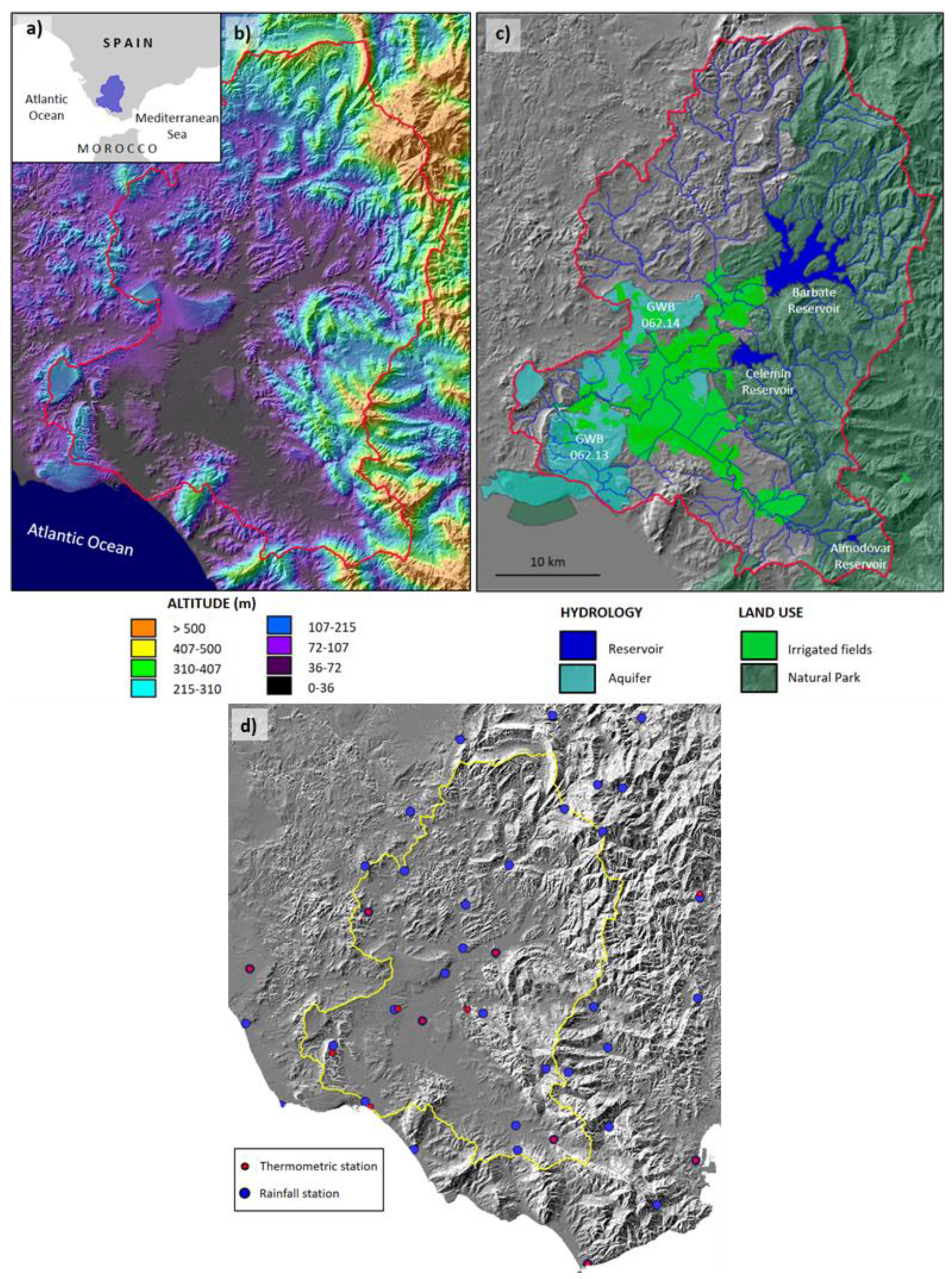
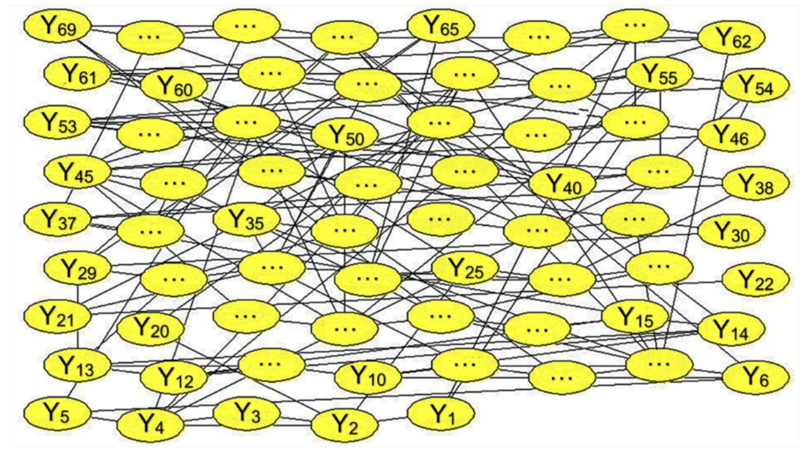
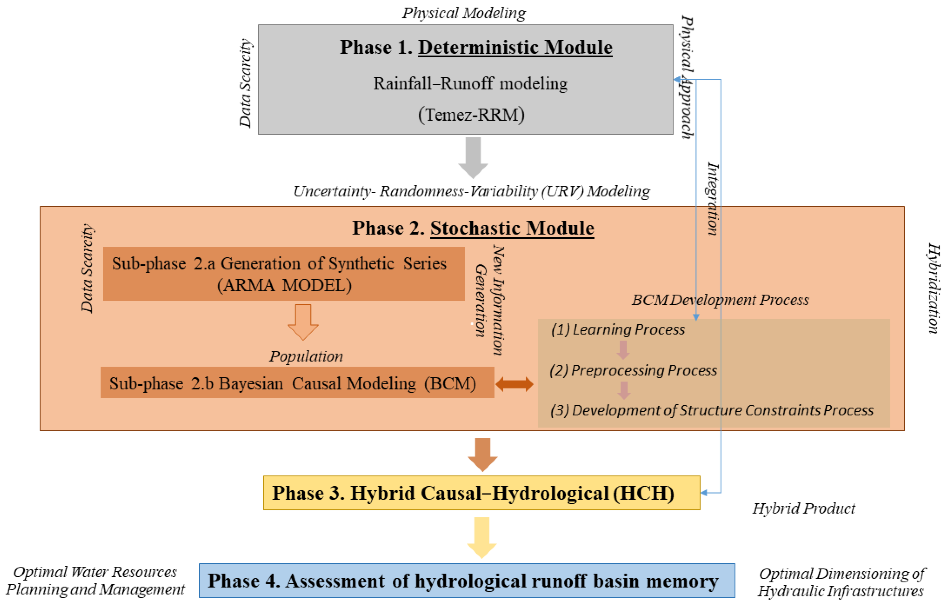
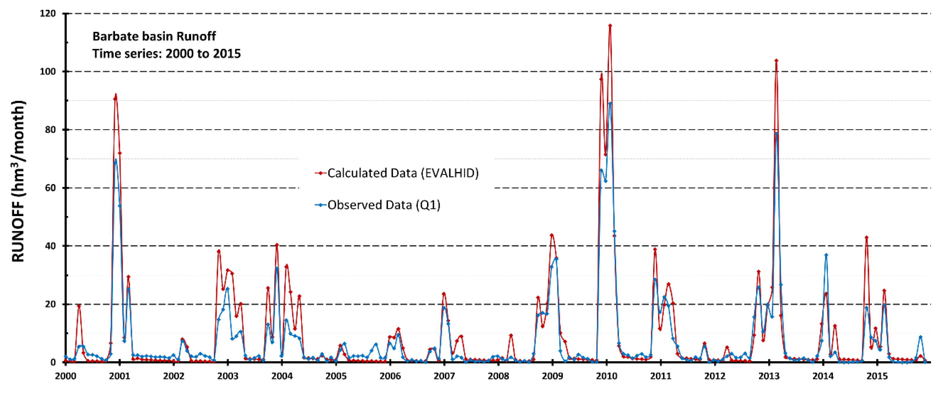
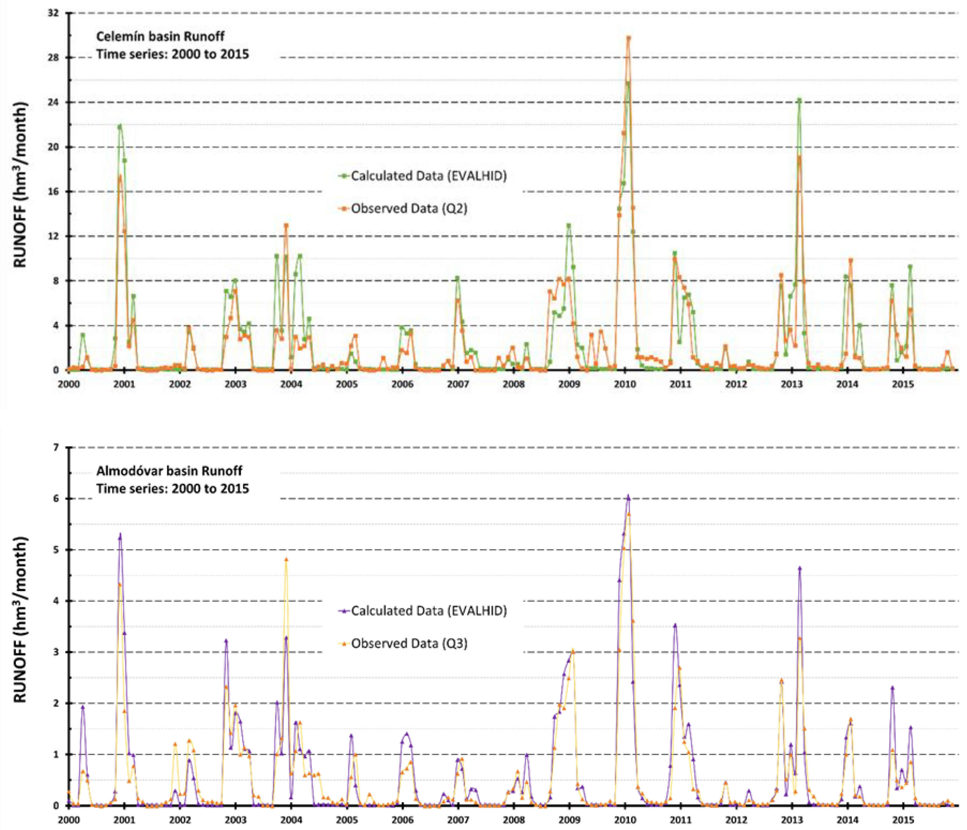
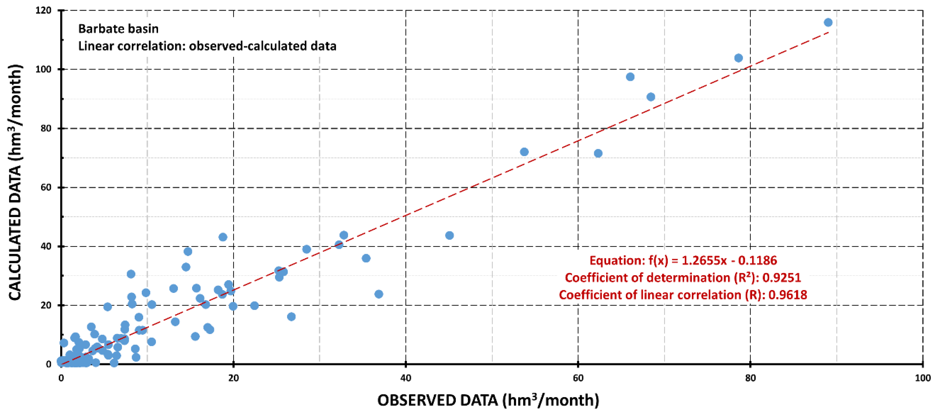
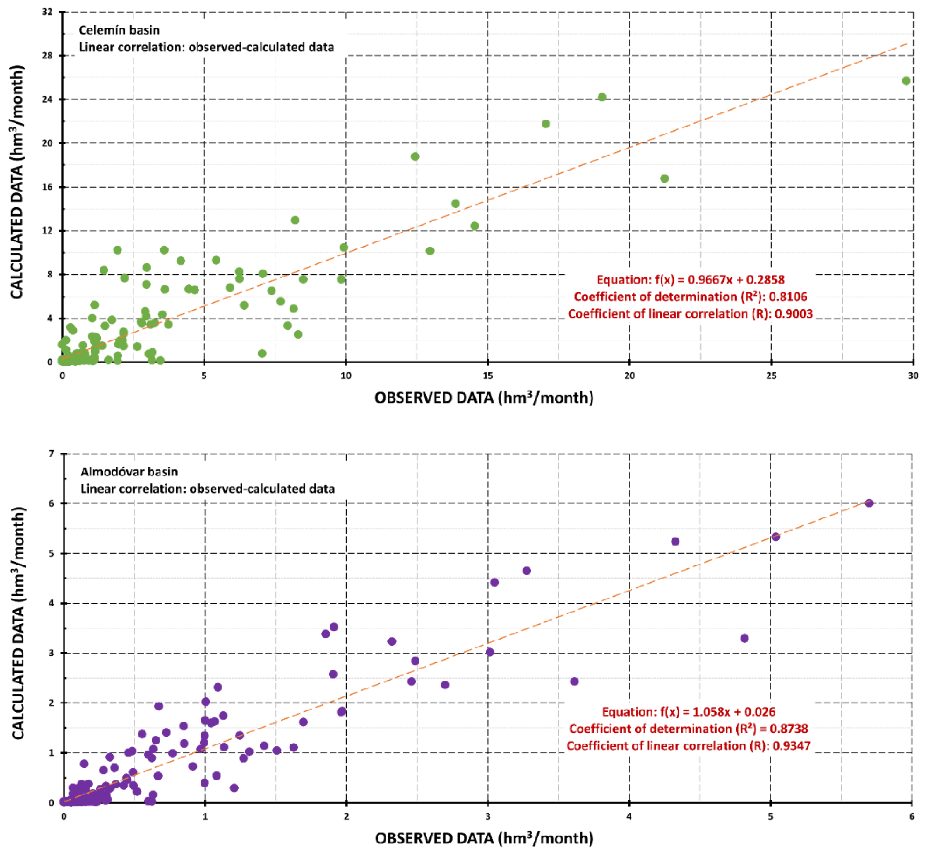
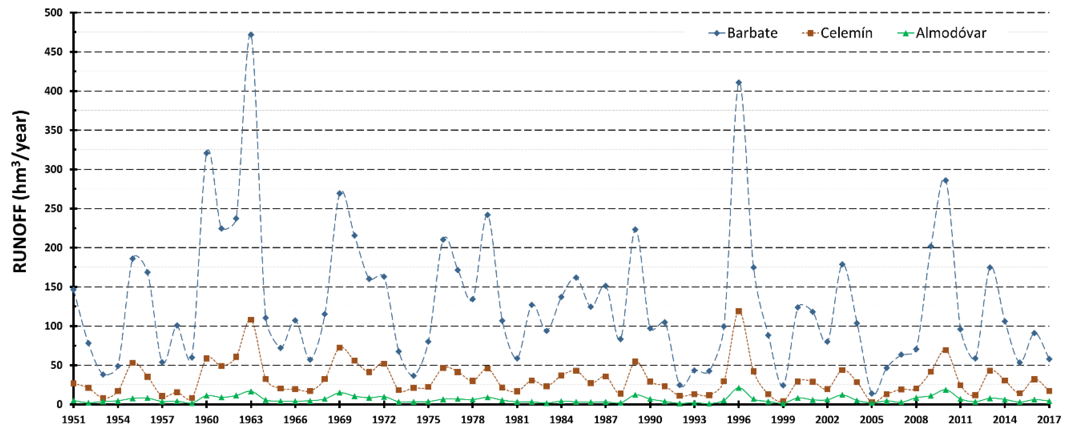
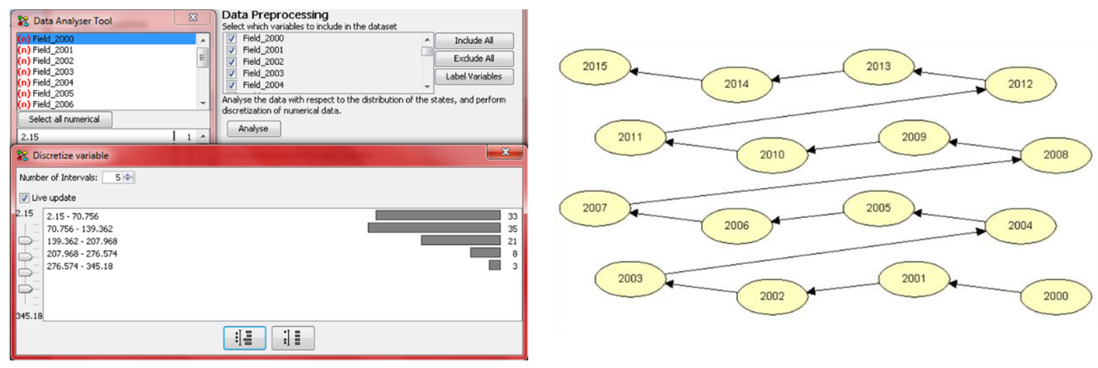
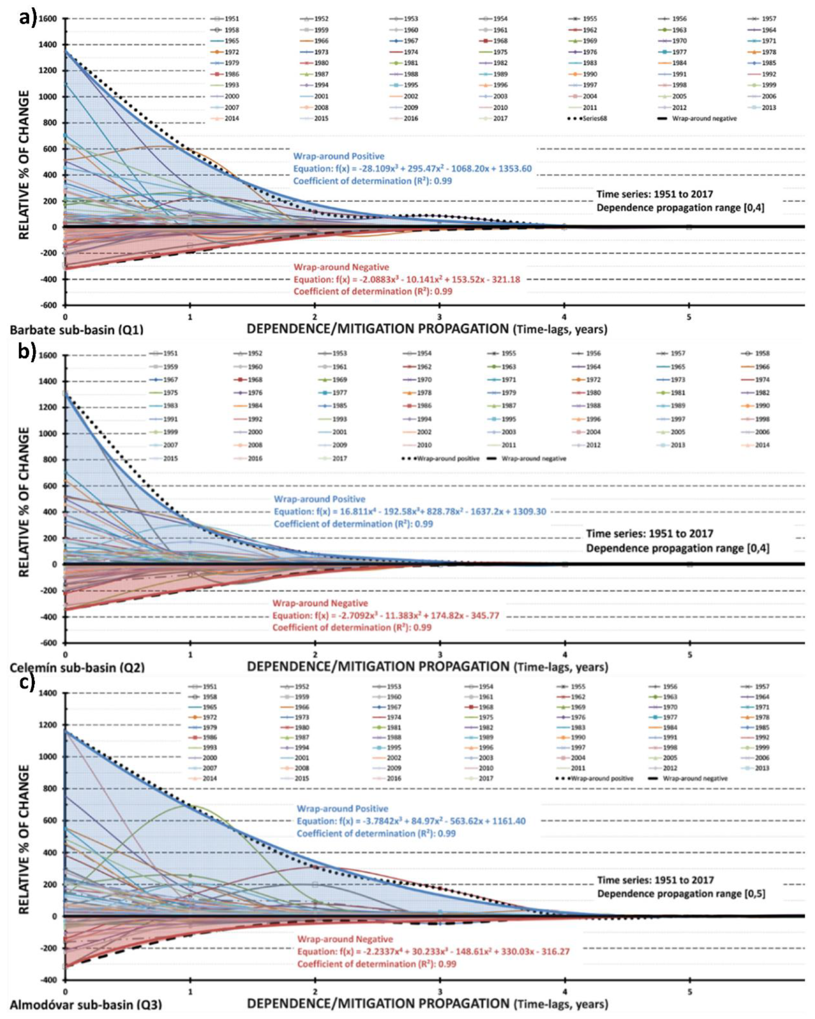
Table 1.
Main morphometric characteristics of the studied sub-basins.
| Sub-Basins/ | Qi 1 | Geological Materials | Extension (Km2) | Elevation (m) | ||||
|---|---|---|---|---|---|---|---|---|
| Code Number | Maximum | Minimum | Mean | Median | ||||
| /1 | Q1 | 2 Flysch. Trias, Jurassic | 149.7 | 1087.4 | 11.3 | 209.1 | 181.2 | |
| Barbate | /2 | Flysch | 59.7 | 1089.6 | 18.0 | 290.2 | 198.9 | |
| /3 | Flysch | 141.8 | 911.8 | 18.0 | 202.2 | 180.9 | ||
| Celemín | /4 | Q2 | Flysch | 94.1 | 630.3 | 19.4 | 196.7 | 185.1 |
| Almodóvar | /5 | Q3 | Flysch | 16.6 | 763.4 | 98.0 | 283.2 | 248.4 |
1 Gauging control points (see Figure 4b). 2 Triassic-Jurassic period.
Table 2.
Parameters after T-RRM calibration.
| Sub-Basin 1/Code Number | Hmax | C | Imax | α (Month−1) |
|---|---|---|---|---|
| /1 | 350 mm | 0.4 | 20 mm | 0.1 |
| Barbate/2 Q1 | 280 mm | 0.3 | 3 mm | 0.1 |
| /3 | 280 mm | 0.3 | 3 mm | 0.1 |
| Celemín/4 Q2 | 280 mm | 0.3 | 3 mm | 0.1 |
| Almodóvar/5 Q3 | 280 mm | 0.3 | 3 mm | 0.1 |
1 Gauging control points (see Figure 4b).
Table 3.
Average monthly and annual runoff values for the Barbate, Celemín, and Almodóvar reservoirs (period: 1951–2017).
Table 3.
Average monthly and annual runoff values for the Barbate, Celemín, and Almodóvar reservoirs (period: 1951–2017).
| Sub-Basins | Month | Average (Hm3) | ||||||||||||
|---|---|---|---|---|---|---|---|---|---|---|---|---|---|---|
| January | February | March | April | May | June | July | August | September | October | November | December | Monthly | Annual | |
| Barbate | 25.0 | 24.5 | 18.8 | 10.5 | 5.5 | 1.2 | 1.0 | 0.9 | 0.9 | 4.2 | 11.3 | 25.2 | 10.8 | 129.1 |
| Celemín | 6.7 | 6.3 | 5.0 | 2.3 | 1.1 | 0.2 | 0.1 | 0.1 | 0.1 | 0.8 | 2.8 | 6.3 | 2.7 | 31.8 |
| Almodóvar | 1.1 | 1.2 | 0.9 | 0.5 | 0.2 | 0.0 | 0.0 | 0.0 | 0.0 | 0.2 | 0.6 | 1.3 | 0.5 | 6.2 |
Table 4.
Main statistical parameters applied in the development of the 9 causal models.
| Sub-Basins 1 | Parameters | T-RRM Results | Average SS 3 | |
|---|---|---|---|---|
| Long series: From 1951 to 2017 | Barbate/Q1 | Mean: | 129.10 Hm3 | 129.71 Hm3 |
| Standard deviation: | 87.78 Hm3 | 93.87 Hm3 | ||
| Skewness coefficient 2: | 1.64 | 1.83 | ||
| Variation coefficient: | 68% | 72% | ||
| Hurst coefficient: | 0.66 | ---------- | ||
| Celemín/Q2 | Mean: | 31.77 Hm3 | 31.89 Hm3 | |
| Standard deviation: | 21.47 Hm3 | 22.39 Hm3 | ||
| Skewness coefficient 2: | 1.84 | 1.73 | ||
| Variation coefficient: | 68% | 70% | ||
| Hurst coefficient: | 0.66 | ---------- | ||
| Almodóvar/Q3 | Mean: | 6.22 Hm3 | 6.16 Hm3 | |
| Standard deviation: | 4.14 Hm3 | 3.92 Hm3 | ||
| Skewness coefficient 2: | 1.54 | 1.42 | ||
| Variation coefficient: | 67% | 64% | ||
| Hurst coefficient: | 0.66 | ---------- | ||
| Sub-basins 1 | Parameters | T-RRM results | Average SS 3 | |
| Short series: From 2000 to 2015 | Barbate/Q1 | Mean: | 110.98 Hm3 | 111.71 Hm3 |
| Standard deviation: | 69.62 Hm3 | 62.46 Hm3 | ||
| Skewness coefficient 2: | 1.13 | 0.58 | ||
| Variation coefficient: | 63% | 56% | ||
| Hurst coefficient: | 0.66 | ---------- | ||
| Celemín/Q2 | Mean: | 27.50 Hm3 | 27.76 Hm3 | |
| Standard deviation: | 16.10 Hm3 | 15.62 Hm3 | ||
| Skewness coefficient 2: | 1.06 | 0.70 | ||
| Variation coefficient: | 59% | 56% | ||
| Hurst coefficient: | 0.61 | ---------- | ||
| Almodóvar/Q3 | Mean: | 7.05 Hm3 | 7.25 Hm3 | |
| Standard deviation: | 4.24 Hm3 | 4.23 Hm3 | ||
| Skewness coefficient 2: | 1.45 | 1.09 | ||
| Variation coefficient: | 60% | 58% | ||
| Hurst coefficient: | 0.69 | ---------- | ||
| Sub-basins 1 | Parameters | Gauging data | Average SS 3 | |
| Short series (Observed data): From 2000 to 2015 | Barbate/Q1 | Mean: | 88.82 Hm3 | 87.83 Hm3 |
| Standard deviation: | 56.08 Hm3 | 52.16 Hm3 | ||
| Skewness coefficient 2: | 1.69 | 1.28 | ||
| Variation coefficient: | 63% | 59% | ||
| 0.74 | ---------- | |||
| Celemín/Q2 | Mean: | 26.58 Hm3 | 28.08 Hm3 | |
| Standard deviation: | 18.54 Hm3 | 20.48 Hm3 | ||
| Skewness coefficient 2: | 1.89 | 1.54 | ||
| Variation coefficient: | 70% | 73% | ||
| 0.77 | ---------- | |||
| Almodóvar/Q3 | Mean: | 6.71 Hm3 | 6.53 Hm3 | |
| Standard deviation: | 4.30 Hm3 | 4.13 Hm3 | ||
| Skewness coefficient 2: | 1.14 | 1.11 | ||
| Variation coefficient: | 64% | 63% | ||
| Hurst coefficient: | 0.57 | ---------- |
1 Gauging Control Point (see Figure 4b). 2 Classic skewness coefficient. 3 Synthetic series from ARMA (1,1).
Publisher’s Note: MDPI stays neutral with regard to jurisdictional claims in published maps and institutional affiliations. |
© 2020 by the authors. Licensee MDPI, Basel, Switzerland. This article is an open access article distributed under the terms and conditions of the Creative Commons Attribution (CC BY) license (http://creativecommons.org/licenses/by/4.0/).
Share and Cite
MDPI and ACS Style
Zazo, S.; Molina, J.-L.; Ruiz-Ortiz, V.; Vélez-Nicolás, M.; García-López, S. Modeling River Runoff Temporal Behavior through a Hybrid Causal–Hydrological (HCH) Method. Water 2020, 12, 3137. https://doi.org/10.3390/w12113137
AMA Style
Zazo S, Molina J-L, Ruiz-Ortiz V, Vélez-Nicolás M, García-López S. Modeling River Runoff Temporal Behavior through a Hybrid Causal–Hydrological (HCH) Method. Water. 2020; 12(11):3137. https://doi.org/10.3390/w12113137
Chicago/Turabian StyleZazo, Santiago, José-Luis Molina, Verónica Ruiz-Ortiz, Mercedes Vélez-Nicolás, and Santiago García-López. 2020. "Modeling River Runoff Temporal Behavior through a Hybrid Causal–Hydrological (HCH) Method" Water 12, no. 11: 3137. https://doi.org/10.3390/w12113137
Note that from the first issue of 2016, this journal uses article numbers instead of page numbers. See further details here.