Implementation of the Kalman Filter for a Geostatistical Bivariate Spatiotemporal Estimation of Hydraulic Conductivity in Aquifers

Abstract

The estimation of the hydraulic parameters of an aquifer such as the hydraulic conductivity is somehow complicated due to its heterogeneity, on the other hand field and laboratory tests are both time consuming and costly. The use of geostatistical-based techniques for data assimilation could represent an alternative tool that allows the use of space-time aquifer behaviour to characterize hydraulic conductivity heterogeneity. In this paper, a spatiotemporal bivariate methodology was implemented combining historical hydraulic head data with hydraulic conductivity sparse data in order to obtain an estimate of the spatial distribution of the latter variable. This approach takes advantage of the correlation between the hydraulic conductivity (K) and the hydraulic head (H) behaviour through time. In order to evaluate this approach, a synthetic experiment was constructed through a transitory numerical flow-model that simulates hydraulic head values in a horizontally-heterogeneous aquifer. Geostatistical tools were used to describe the correlation between simulated spatiotemporal data of hydraulic head and the spatial distribution of the hydraulic conductivity in a group of model nodes. Subsequently, the Kalman filter was used to estimate the hydraulic conductivity values at nonsampled sites. The results showed acceptable differences between estimated and synthetic hydraulic conductivity data, with low estimate error variances (predominating the 1 m²/day² value for K for all the cases, however, the smallest number of cells with values above 2 m²/day² correspond to the bivariate spatiotemporal case) and the best agreement between the estimated errors and the selected model variance (SMSE values of 0.574 and 0.469) were found for the bivariate cases, which suggests that the implemented methodology could be used for reducing calibration efforts, particularly when the hydraulic parameters data are scarce.

1. Introduction

Hydraulic conductivity (K) represents a fundamental parameter in the drainage and irrigation systems design, agricultural engineering, soil science and industry, among others [1,2,3]. Other applications can be found in construction and building materials; some other examples of infrastructures where the K is essential are heat-insulation walls, permeable embankments, soil barriers, and backfill engineering on soft ground [4,5,6]. Zhong et al. [7] proposed a modification to an existing model in order to improve the K prediction with measured data in pervious concrete taking into account the pore size and tortuosity. Turco et al. [8] calibrated a reservoir element model with experimental data of different rain falls (water retention curve and saturated hydraulic conductivity) on an experimental five layers permeable pavement.

On the other hand, there are many applications referred to the use of the K for estimating groundwater yield and prospection, groundwater flow, contaminant transport dynamics and soil electrical characteristics [9,10,11]. For example, Luo et al. [12] presented a method based on the effective groundwater drainage length concept and a dynamic equilibrium condition for predicting the K in a northwest USA valley with similar results to those obtained in previous works at a few observation points. Brunetti et al. [13] used data from a Cosmic-Ray Neutron probe to inversely estimate the soil hydraulic properties such as the hydraulic conductivity and the volumetric water content on a 200 cm deep homogeneous loamy sand soil profile covered by grass. Hörning et al. [14] presented a modification of a geostatistical simulation technique based on Monte Carlo approach in order to reduce the computational cost in the calibration phase using two groundwater examples. Different variables such as the hydraulic head, transmissivity and conductivity were used for inverse modelling.

Numerical flow models are considered as one of the most reliable methods to evaluate groundwater resources; for its construction, it is necessary to specify the lateral and vertical spatial aquifer limits, the initial and boundary conditions (including recharge and discharge, whether it is natural or artificial) as well as the K and the storage coefficient.

In flow modelling, reliable and known hydraulic parameters are required; however, these data are commonly scarce and presented a high spatial variability due to the local properties heterogeneity for each geological system. These values are usually obtained on-site from aquifer tests (by pumping, which provide the most representative values for field conditions), in laboratories through permeability tests, or alternatively from reference tables. Batlle-Aguilar et al. [15] reviewed some hydraulic and chemical methods in order to estimate K and the porewater velocity. Likewise, geoelectrical methods have been used for the estimation of the hydraulic conductivity since they are relatively faster and cheaper than other tests.

The estimation of the aquifer hydraulic parameters through on-site tests are representative only for a limited area around the pumping well used, besides, its inherent execution cost and field implementation difficulties. On the other hand, the values estimated from laboratory permeability tests do not reflect the aquifer field conditions. Another possibility is to use the values from reference tables that presented ranges for different geological materials but it is not easy to select an appropriate value for a specific aquifer because of its several materials. This estimation can be complemented with resistivity data in areas where the information revealed by the wells and the pumping tests are not enough, or even missing [16]. Another proposal for estimating soils’ hydraulic conductivity is the use of pedotransfer functions [17].

As an alternative, different calibration methods are used to predict the hydraulic parameters of a groundwater model, the selection of the method depends on the study approach. For a manual model calibration, the boundary conditions must be established in order to minimize the differences between simulated and observed values. If the conceptual model or the initial and boundary conditions are not properly defined, it is highly probable that the estimated hydraulic parameters will be far from reality after the calibration process. In the calibration stage, the use of an optimization algorithm is essential to minimize the objective function. Besides, different spatial distributions of the hydraulic parameters (between predefined lower and upper limits) are proposed, so the procedure usually requires repeatedly evaluating the objective function till the lowest error between observed–predicted values is found [18]. Some other approaches have focused on the deterministic inverse approach considering the solute transport parameters [19].

The conditioning problem for direct measurements has been addressed to geostatistics through data assimilation, which refers to the process of combining a prediction model of a state variable with a set of discrete measurements [20]. The objective of data assimilation, in the context of inverse modelling, is to estimate a random field of state variables, extracting or filtering as much information as possible from noisy observations, leading to the best possible statistical estimation of the variable field.

Spatial interpolation methods such as kriging are frequently used to estimate the spatial distribution of hydraulic conductivity (K) at nonsampled locations based on scarce data. Geostatistical methods based on spatial correlation do not give good results at model validation [21]. For that reason, some authors have solved the inverse problem by obtaining the K distribution based on secondary variables. Inverse modelling generates valuable data mainly when the analysed variable is scarce and heterogeneous.

The Kalman filter (KF) has been widely used in different fields of science, it allows obtaining, through a recursive procedure, linear unbiased estimates with a minimum variance for the state of a system using noisy data [22]. If the dynamic system is nonlinear, it is possible to use modifications of the Kalman filter (i.e., Extended Kalman filter (EKF), Ensemble Kalman filter (EnKF) [23] or Ensemble Smoother (ES) [24,25]). Monte Carlo (MC) simulation is used in both EnKF and ES to define the state vector. In the Herrera’s thesis [25], ES was applied for solving groundwater problems in parameters estimation. Bailey and Baù [26] estimated the hydraulic conductivity through ES using two variables: hydraulic head data and flow returns. The EnKF based on a Bayesian sequential update rule produces similar results to those obtained by MC but with a significantly shorter computational time due to its flexibility for incorporating multiple sources of uncertainty [27,28]. Franssen and Kinzelbach [29] analysed a synthetic groundwater case with two variables (recharge rate and transmissivity) and demonstrated that the EnKF requires 80% less computation time than the inverse modelling methods. Due to the robustness of the EnKF against nonlinearity systems of the state transition function, it has been successfully used for modelling groundwater flow and transport [20]. Several applications of the EnKF can be found in the literature to simultaneously estimate the hydraulic parameters, the hydraulic head and, in some cases contaminant concentrations within aquifers by using numerical flow and transport models [29,30,31,32,33,34,35]. Before any calibration effort, it is desirable to have a good initial spatial distribution of the hydraulic parameters; therefore, different estimation methods have been implemented (univariate and bivariate geostatistical techniques).

The objective of this paper was to implement a bivariate spatiotemporal geostatistical-based methodology that combines spatiotemporal hydraulic head data with hydraulic conductivity (K) sparse data in order to obtain the spatial distribution of K. Covariances were strictly derived from geostatistical analyses, not from numerical flow model simulations. This approach was compared with estimated values using univariate (hydraulic conductivity data only) and spatial bivariate (hydraulic conductivity as the main variable and hydraulic head data for a single time as secondary variable) geostatistical approaches.

2. Materials and Methods

In order to evaluate the performance of the proposed approach to estimate hydraulic conductivity, data from a synthetic numerical flow model was used. It was assumed that in some cells of the model, hydraulic conductivity values were available, then, a geostatistical analysis was done with these data to estimate hydraulic conductivity in the remaining cells employing the static Kalman filter as estimator. In this manner, it was possible to evaluate the proposed approach by comparing the model input data and the estimated K values.

Even though the traditional estimation of univariate and bivariate cases is done with kriging interpolation, in the case study, the Kalman filter is used as the estimation method due to its ease to incorporate the bivariate spatiotemporal case.

The hydraulic conductivity was estimated by three different geostatistical-based methods:

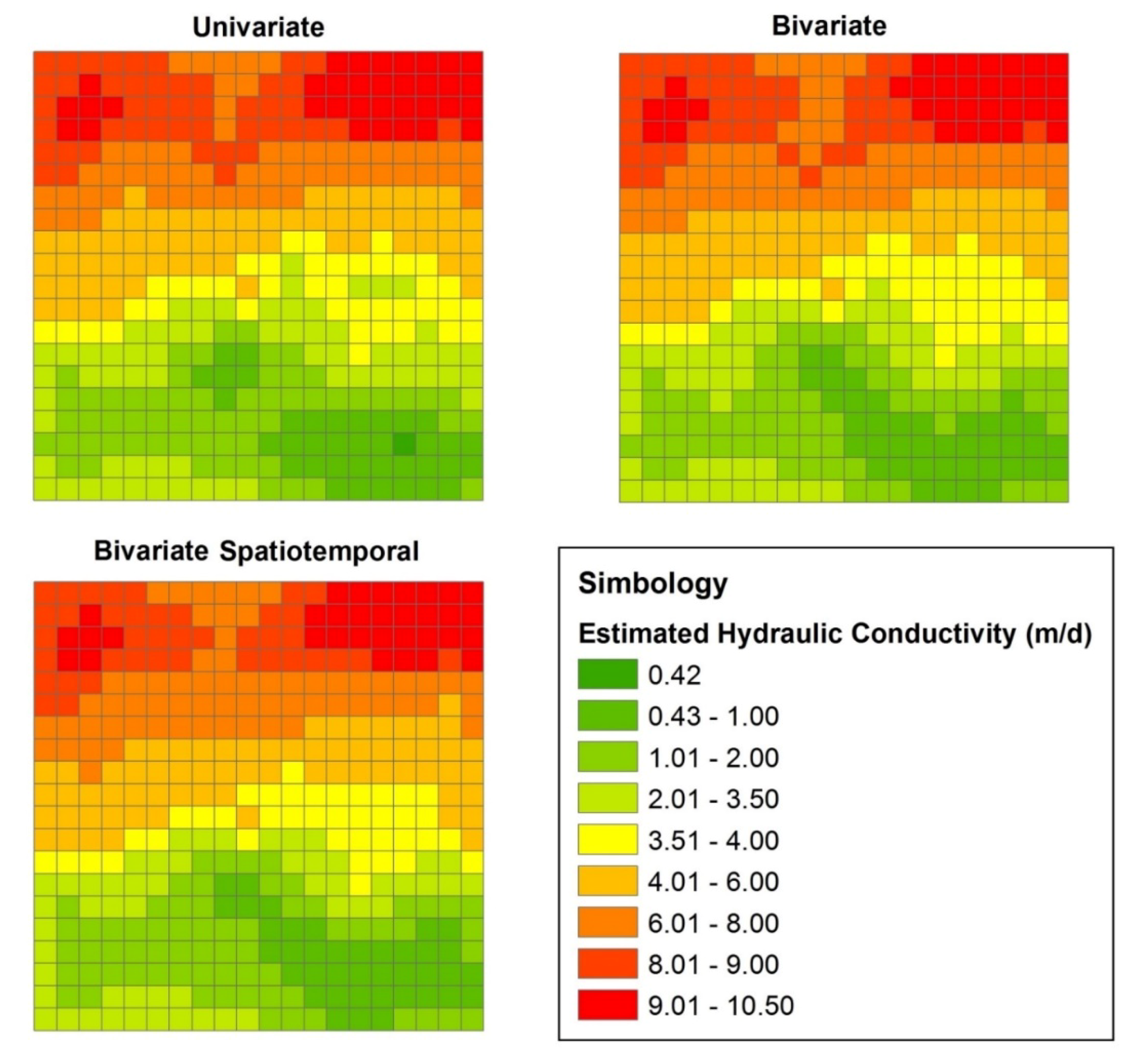
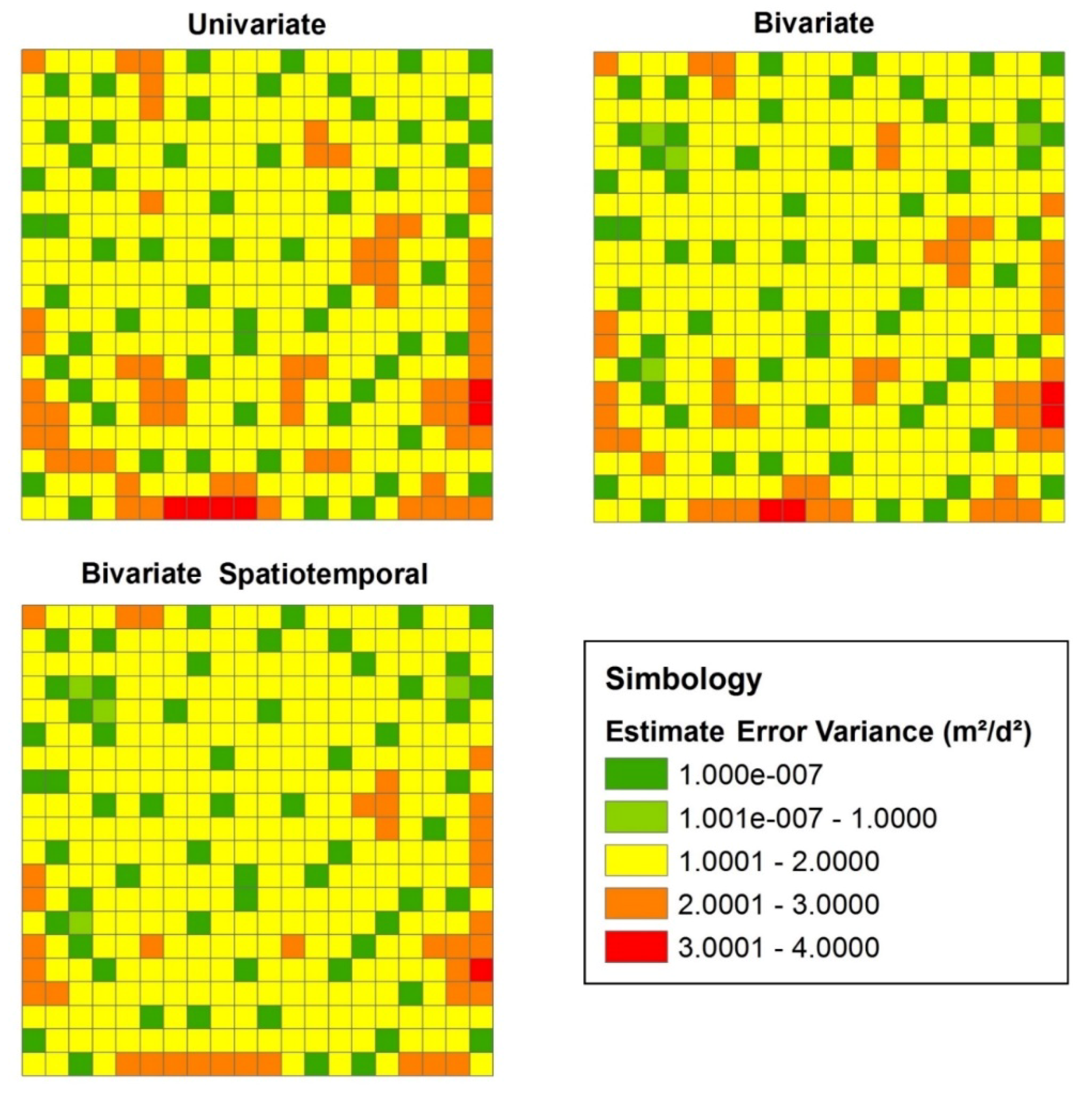
• Univariate estimation (based on the spatial correlation of hydraulic conductivity data only).
• Bivariate or cross estimation (hydraulic conductivity as the primary variable and hydraulic head for a single time as the secondary).
• Multivariate spatiotemporal estimation (based on the correlation between the hydraulic conductivity data and the hydraulic head spatiotemporal data).

In the following subsections, a description of the geostatistical procedure to derive the univariate, cross and spatiotemporal covariance matrices is presented, then, the scheme for the multivariable covariance matrix is shown. Finally, relevant aspects of the Kalman filter theory and its implementation for the proposed methodology are included.

2.1. Geostatistical Theory

Geostatistical analyses were followed in order to determine the spatial, cross and spatiotemporal structures of covariance matrices derived from variograms.

The sampling variograms were defined as follows:

2.1.1. The Spatial Variogram

The sample variogram is calculated with:

$${\mathsf{\gamma }}_{\mathrm{s}}^{*}=\frac{1}{2\mathrm{N}\left(\mathrm{h}\right)}{{\displaystyle \sum }}_{\mathrm{i}=1}^{\mathrm{N}\left(\mathrm{h}\right)}{\left[\mathrm{Z}\left({\mathrm{x}}_{\mathrm{i}}\right)-\mathrm{Z}\left({\mathrm{x}}_{\mathrm{i}}+\mathrm{h}\right)\right]}^2,$$

(1)

where N(h) is the number of pairs, Z(x_i) and Z(x_i + h) are the tail and head values, respectively. i is the position of coordinates (x_i, y_i). The separation vector h is specified with some direction and distance (lag) tolerance [36].

When the variogram model is selected, the covariance matrix can be derived by using the following property for a second-order stationary spatial random field:

$${\mathrm{C}}_{\mathrm{s}}\left({\mathrm{h}}_{\mathrm{s}}\right)={\mathrm{C}}_{\mathrm{s}}\left(0\right)-{\mathsf{\gamma }}_{\mathrm{s}}\left({\mathrm{h}}_{\mathrm{s}}\right),$$

(2)

where ${\mathrm{C}}_{\mathrm{s}}\left({\mathrm{h}}_{\mathrm{s}}\right)$ is the spatial covariance, ${\mathrm{C}}_{\mathrm{s}}\left(0\right)$ is the variance and ${\mathsf{\gamma }}_{\mathrm{s}}\left({\mathrm{h}}_{\mathrm{s}}\right)$ is the spatial variogram model. ${\mathrm{h}}_{\mathrm{s}}$ is the spatial distance between two positions of the covariance matrix. The structure of the spatial covariance matrix is shown in

Table 1. Structure of the univariate spatial covariance matrix.

$\mathrm{C}\left({\mathrm{x}}_{\mathrm{i}},{\mathrm{x}}_{\mathrm{i}}\right)$	$\mathrm{C}\left({\mathrm{x}}_{\mathrm{i}},{\mathrm{x}}_{\mathrm{i}+1}\right)$	$\dots$	$\mathrm{C}\left({\mathrm{x}}_{\mathrm{i}},{\mathrm{x}}_{\mathrm{N}}\right)$
$\mathrm{C}\left({\mathrm{x}}_{\mathrm{i}+1},{\mathrm{x}}_{\mathrm{i}}\right)$	$\mathrm{C}\left({\mathrm{x}}_{\mathrm{i}+1},{\mathrm{x}}_{\mathrm{i}+1}\right)$	$\dots$	$\mathrm{C}\left({\mathrm{x}}_{\mathrm{i}+1},{\mathrm{x}}_{\mathrm{N}}\right)$
⋮	⋮	⋮	⋮
$\mathrm{C}\left({\mathrm{x}}_{\mathrm{N}},{\mathrm{x}}_{\mathrm{i}}\right)$	$\mathrm{C}\left({\mathrm{x}}_{\mathrm{N},}{\mathrm{x}}_{\mathrm{i}+1}\right)$	$\dots$	$\mathrm{C}\left({\mathrm{x}}_{\mathrm{N}},{\mathrm{x}}_{\mathrm{N}}\right)$

.

2.1.2. The Cross Variogram

The sample cross-variogram for variables $\mathrm{Z}$ and $\mathrm{Y}$ is:

$${\mathsf{\gamma }}_{\mathrm{ZY}}^{*}\left(\mathrm{h}\right)=\frac{1}{2\mathrm{N}\left(\mathrm{h}\right)}{{\displaystyle \sum }}_{\mathrm{i}=1}^{\mathrm{N}\left(\mathrm{h}\right)}\left[\mathrm{Z}\left({\mathrm{x}}_{\mathrm{i}}\right)-\mathrm{Z}\left({\mathrm{x}}_{\mathrm{i}}+\mathrm{h}\right)\right]\left[\mathrm{Y}\left({\mathrm{x}}_{\mathrm{i}}\right)-\mathrm{Y}\left({\mathrm{x}}_{\mathrm{i}}+\mathrm{h}\right)\right],$$

(3)

For second-order stationary processes, the cross-covariance and the pseudo-cross-variogram are related with Webster and Oliver [37]:

$${\mathrm{C}}_{\mathrm{ZY}}\left(\mathrm{h}\right)=\frac{1}{2}\left\{{\mathrm{C}}_{\mathrm{ZZ}}\left(0\right)+{\mathrm{C}}_{\mathrm{YY}}\left(0\right)\right\}-{\mathsf{\gamma }}_{\mathrm{ZY}}^{\mathrm{P}}\left(\mathrm{h}\right)$$

(4)

The structure of the cross covariance is shown in

Table 2. Structure of the cross-covariance matrix.

${\mathrm{C}}_{\mathrm{ZY}}\left({\mathrm{x}}_{\mathrm{i}},{\mathrm{x}}_{\mathrm{i}}\right)$	${\mathrm{C}}_{\mathrm{ZY}}\left({\mathrm{x}}_{\mathrm{i}},{\mathrm{x}}_{\mathrm{i}+1}\right)$	$\dots$	${\mathrm{C}}_{\mathrm{ZY}}\left({\mathrm{x}}_{\mathrm{i}},{\mathrm{x}}_{\mathrm{N}}\right)$
${\mathrm{C}}_{\mathrm{ZY}}\left({\mathrm{x}}_{\mathrm{i}+1},{\mathrm{x}}_{\mathrm{i}}\right)$	${\mathrm{C}}_{\mathrm{ZY}}\left({\mathrm{x}}_{\mathrm{i}+1},{\mathrm{x}}_{\mathrm{i}+1}\right)$	$\dots$	${\mathrm{C}}_{\mathrm{ZY}}\left({\mathrm{x}}_{\mathrm{i}+1},{\mathrm{x}}_{\mathrm{N}}\right)$
⋮	⋮	⋮	⋮
${\mathrm{C}}_{\mathrm{ZY}}\left({\mathrm{x}}_{\mathrm{N}},{\mathrm{x}}_{\mathrm{i}}\right)$	${\mathrm{C}}_{\mathrm{ZY}}\left({\mathrm{x}}_{\mathrm{N},}{\mathrm{x}}_{\mathrm{i}+1}\right)$	$\dots$	${\mathrm{C}}_{\mathrm{ZY}}\left({\mathrm{x}}_{\mathrm{N}},{\mathrm{x}}_{\mathrm{N}}\right)$

.

2.1.3. The Spatiotemporal Variogram

In the space–time conceptualization, the sample variogram for the spatial and temporal lags (h_s and h_t, respectively) is based on the following expression:

$${\mathsf{\gamma }}_{\mathrm{st}}^{*}({\mathrm{h}}_{\mathrm{s}},{\mathrm{h}}_{\mathrm{t}})=\frac{1}{2\mathrm{N}({\mathrm{h}}_{\mathrm{s}},{\mathrm{h}}_{\mathrm{t}})}{{\displaystyle \sum }}_{\mathrm{i}=1}^{\mathrm{T}}{{\displaystyle \sum }}_{\mathrm{k}=1}^{\mathrm{N}({\mathrm{h}}_{\mathrm{s}},{\mathrm{h}}_{\mathrm{t}})}{\left[\mathrm{Z}\left({\mathrm{x}}_{\mathrm{k}},{\mathrm{t}}_{\mathrm{i}}\right)-\mathrm{Z}\left({\mathrm{x}}_{\mathrm{k}}+{\mathrm{h}}_{\mathrm{s}},{\mathrm{t}}_{\mathrm{i}}+{\mathrm{h}}_{\mathrm{t}}\right)\right]}^2,$$

(5)

where N(h_s,h_t) is the number of pairs Z(x_i,t_k) and Z(x_i + h_s,t_k + h_t) separated by increments h_s and h_t, T is the total number of times with data. h_t is the temporal distance between two spatiotemporal positions.

In an analogue way to the spatial case, the spatiotemporal covariance matrix is derived from the following equation for a second-order stationary space-time random field [38]:

$${\mathrm{C}}_{\mathrm{st}}\left({\mathrm{h}}_{\mathrm{s}},{\mathrm{h}}_{\mathrm{t}}\right)={\mathrm{C}}_{\mathrm{st}}\left(0,0\right)-{\mathsf{\gamma }}_{\mathrm{st}}\left({\mathrm{h}}_{\mathrm{s}},{\mathrm{h}}_{\mathrm{t}}\right)$$

(6)

The structure of the derived space-time covariance is as shown in

Table 3. Structure of the space–time covariance matrix.

$\mathrm{C}\left({\mathrm{x}}_{\mathrm{i},\mathrm{t}},{\mathrm{x}}_{\mathrm{i},\mathrm{t}}\right)$

$\mathrm{C}\left({\mathrm{x}}_{\mathrm{i},\mathrm{t}},{\mathrm{x}}_{\mathrm{i}+1,\mathrm{t}}\right)$

…

$\mathrm{C}\left({\mathrm{x}}_{\mathrm{i},\mathrm{t}},{\mathrm{x}}_{\mathrm{NP},\mathrm{t}}\right)$

$\mathrm{C}\left({\mathrm{x}}_{\mathrm{i},\mathrm{t}},{\mathrm{x}}_{\mathrm{i},\mathrm{t}+1}\right)$

$\mathrm{C}\left({\mathrm{x}}_{\mathrm{i},\mathrm{t}},{\mathrm{x}}_{\mathrm{i}+1,\mathrm{t}+1}\right)$

…

$\mathrm{C}\left({\mathrm{x}}_{\mathrm{i},\mathrm{t}},{\mathrm{x}}_{\mathrm{NP},\mathrm{t}+1}\right)$

…

$\mathrm{C}\left({\mathrm{x}}_{\mathrm{i},\mathrm{t}},{\mathrm{x}}_{\mathrm{i},\mathrm{NT}}\right)$

$\mathrm{C}\left({\mathrm{x}}_{\mathrm{i},\mathrm{t}},{\mathrm{x}}_{\mathrm{i}+1,\mathrm{NT}}\right)$

…

$\mathrm{C}\left({\mathrm{x}}_{\mathrm{i},\mathrm{t}},{\mathrm{x}}_{\mathrm{NP},\mathrm{NT}}\right)$

$\mathrm{C}\left({\mathrm{x}}_{\mathrm{i}+1,\mathrm{t}},{\mathrm{x}}_{\mathrm{i},\mathrm{t}}\right)$

$\mathrm{C}\left({\mathrm{x}}_{\mathrm{i}+1,\mathrm{t}},{\mathrm{x}}_{\mathrm{i}+1,\mathrm{t}}\right)$

…

$\mathrm{C}\left({\mathrm{x}}_{\mathrm{i},\mathrm{t}},{\mathrm{x}}_{\mathrm{NP},\mathrm{t}}\right)$

$\mathrm{C}\left({\mathrm{x}}_{\mathrm{i}+1,\mathrm{t}},{\mathrm{x}}_{\mathrm{i},\mathrm{t}+1}\right)$

$\mathrm{C}\left({\mathrm{x}}_{\mathrm{i}+1,\mathrm{t}},{\mathrm{x}}_{\mathrm{i}+1,\mathrm{t}+1}\right)$

…

$\mathrm{C}\left({\mathrm{x}}_{\mathrm{i}+1,\mathrm{t}},{\mathrm{x}}_{\mathrm{NP},\mathrm{t}+1}\right)$

…

$\mathrm{C}\left({\mathrm{x}}_{\mathrm{i}+1,\mathrm{t}},{\mathrm{x}}_{\mathrm{i},\mathrm{NT}}\right)$

$\mathrm{C}\left({\mathrm{x}}_{\mathrm{i}+1,\mathrm{t}},{\mathrm{x}}_{\mathrm{i}+1,\mathrm{NT}}\right)$

…

$\mathrm{C}\left({\mathrm{x}}_{\mathrm{i}+1,\mathrm{t}},{\mathrm{x}}_{\mathrm{NP},\mathrm{NT}}\right)$

⋮

⋮

⋮

⋮

⋮

⋮

⋮

⋮

⋮

⋮

⋮

⋮

⋮

$\mathrm{C}\left({\mathrm{x}}_{\mathrm{NP},\mathrm{t}},{\mathrm{x}}_{\mathrm{i},\mathrm{t}}\right)$

$\mathrm{C}\left({\mathrm{x}}_{\mathrm{NP},\mathrm{t}},{\mathrm{x}}_{\mathrm{i}+1,\mathrm{t}}\right)$

…

$\mathrm{C}\left({\mathrm{x}}_{\mathrm{NP},\mathrm{t}},{\mathrm{x}}_{\mathrm{NP},\mathrm{t}}\right)$

$\mathrm{C}\left({\mathrm{x}}_{\mathrm{NP},\mathrm{t}},{\mathrm{x}}_{\mathrm{i},\mathrm{t}+1}\right)$

$\mathrm{C}\left({\mathrm{x}}_{\mathrm{NP},\mathrm{t}},{\mathrm{x}}_{\mathrm{i}+1,\mathrm{t}+1}\right)$

…

$\mathrm{C}\left({\mathrm{x}}_{\mathrm{NP},\mathrm{t}},{\mathrm{x}}_{\mathrm{NP},\mathrm{t}+1}\right)$

…

$\mathrm{C}\left({\mathrm{x}}_{\mathrm{NP},\mathrm{t}},{\mathrm{x}}_{\mathrm{i},\mathrm{NT}}\right)$

$\mathrm{C}\left({\mathrm{x}}_{\mathrm{NP},\mathrm{t}},{\mathrm{x}}_{\mathrm{i}+1,\mathrm{NT}}\right)$

…

$\mathrm{C}\left({\mathrm{x}}_{\mathrm{NP},\mathrm{t}},{\mathrm{x}}_{\mathrm{NP},\mathrm{NT}}\right)$

$\mathrm{C}\left({\mathrm{x}}_{\mathrm{i},\mathrm{t}+1},{\mathrm{x}}_{\mathrm{i},\mathrm{t}}\right)$

$\mathrm{C}\left({\mathrm{x}}_{\mathrm{i},\mathrm{t}+1},{\mathrm{x}}_{\mathrm{i}+1,\mathrm{t}}\right)$

…

$\mathrm{C}\left({\mathrm{x}}_{\mathrm{i},\mathrm{t}+1},{\mathrm{x}}_{\mathrm{NP},\mathrm{t}}\right)$

$\mathrm{C}\left({\mathrm{x}}_{\mathrm{i},\mathrm{t}+1},{\mathrm{x}}_{\mathrm{i},\mathrm{t}+1}\right)$

$\mathrm{C}\left({\mathrm{x}}_{\mathrm{i},\mathrm{t}+1},{\mathrm{x}}_{\mathrm{i}+1,\mathrm{t}+1}\right)$

…

$\mathrm{C}\left({\mathrm{x}}_{\mathrm{i},\mathrm{t}+1},{\mathrm{x}}_{\mathrm{NP},\mathrm{t}+1}\right)$

…

$\mathrm{C}\left({\mathrm{x}}_{\mathrm{i},\mathrm{t}+1},{\mathrm{x}}_{\mathrm{i},\mathrm{NT}}\right)$

$\mathrm{C}\left({\mathrm{x}}_{\mathrm{i},\mathrm{t}+1},{\mathrm{x}}_{\mathrm{i}+1,\mathrm{NT}}\right)$

…

$\mathrm{C}\left({\mathrm{x}}_{\mathrm{i},\mathrm{t}+1},{\mathrm{x}}_{\mathrm{NP},\mathrm{NT}}\right)$

$\mathrm{C}\left({\mathrm{x}}_{\mathrm{i}+1,\mathrm{t}+1},{\mathrm{x}}_{\mathrm{i},\mathrm{t}}\right)$

$\mathrm{C}\left({\mathrm{x}}_{\mathrm{i}+1,\mathrm{t}+1},{\mathrm{x}}_{\mathrm{i}+1,\mathrm{t}}\right)$

…

$\mathrm{C}\left({\mathrm{x}}_{\mathrm{i}+1,\mathrm{t}+1},{\mathrm{x}}_{\mathrm{NP},\mathrm{t}}\right)$

$\mathrm{C}\left({\mathrm{x}}_{\mathrm{i}+1,\mathrm{t}+1},{\mathrm{x}}_{\mathrm{i},\mathrm{t}+1}\right)$

$\mathrm{C}\left({\mathrm{x}}_{\mathrm{i}+1,\mathrm{t}+1},{\mathrm{x}}_{\mathrm{i}+1,\mathrm{t}+1}\right)$

…

$\mathrm{C}\left({\mathrm{x}}_{\mathrm{i}+1,\mathrm{t}+1},{\mathrm{x}}_{\mathrm{NP},\mathrm{t}+1}\right)$

…

$\mathrm{C}\left({\mathrm{x}}_{\mathrm{i}+1,\mathrm{t}+1},{\mathrm{x}}_{\mathrm{i},\mathrm{NT}}\right)$

$\mathrm{C}\left({\mathrm{x}}_{\mathrm{i}+1,\mathrm{t}+1},{\mathrm{x}}_{\mathrm{i}+1,\mathrm{NT}}\right)$

…

$\mathrm{C}\left({\mathrm{x}}_{\mathrm{i}+1,\mathrm{t}+1},{\mathrm{x}}_{\mathrm{NP},\mathrm{NT}}\right)$

⋮

⋮

⋮

⋮

⋮

⋮

⋮

⋮

⋮

⋮

⋮

⋮

⋮

$\mathrm{C}\left({\mathrm{x}}_{\mathrm{NP},\mathrm{t}+1},{\mathrm{x}}_{\mathrm{i},\mathrm{t}}\right)$

$\mathrm{C}\left({\mathrm{x}}_{\mathrm{NP},\mathrm{t}+1},{\mathrm{x}}_{\mathrm{i}+1,\mathrm{t}}\right)$

…

$\mathrm{C}\left({\mathrm{x}}_{\mathrm{NP},\mathrm{t}+1},{\mathrm{x}}_{\mathrm{NP},\mathrm{t}}\right)$

$\mathrm{C}\left({\mathrm{x}}_{\mathrm{NP},\mathrm{t}+1},{\mathrm{x}}_{\mathrm{i},\mathrm{t}+1}\right)$

$\mathrm{C}\left({\mathrm{x}}_{\mathrm{NP},\mathrm{t}+1},{\mathrm{x}}_{\mathrm{i}+1,\mathrm{t}+1}\right)$

…

$\mathrm{C}\left({\mathrm{x}}_{\mathrm{NP},\mathrm{t}+1},{\mathrm{x}}_{\mathrm{NP},\mathrm{t}+1}\right)$

…

$\mathrm{C}\left({\mathrm{x}}_{\mathrm{NP},\mathrm{t}+1},{\mathrm{x}}_{\mathrm{i},\mathrm{NT}}\right)$

$\mathrm{C}\left({\mathrm{x}}_{\mathrm{NP},\mathrm{t}+1},{\mathrm{x}}_{\mathrm{i}+1,\mathrm{NT}}\right)$

…

$\mathrm{C}\left({\mathrm{x}}_{\mathrm{NP},\mathrm{t}+1},{\mathrm{x}}_{\mathrm{NP},\mathrm{NT}}\right)$

⋮

⋮

⋮

⋮

⋮

⋮

⋮

⋮

⋮

⋮

⋮

⋮

⋮

$\mathrm{C}\left({\mathrm{x}}_{\mathrm{i},\mathrm{NT}},{\mathrm{x}}_{\mathrm{i},\mathrm{t}}\right)$

$\mathrm{C}\left({\mathrm{x}}_{\mathrm{i},\mathrm{NT}},{\mathrm{x}}_{\mathrm{i}+1,\mathrm{t}}\right)$

…

$\mathrm{C}\left({\mathrm{x}}_{\mathrm{i},\mathrm{NT}},{\mathrm{x}}_{\mathrm{NP},\mathrm{t}}\right)$

$\mathrm{C}\left({\mathrm{x}}_{\mathrm{i},\mathrm{NT}},{\mathrm{x}}_{\mathrm{i},\mathrm{t}+1}\right)$

$\mathrm{C}\left({\mathrm{x}}_{\mathrm{i},\mathrm{NT}},{\mathrm{x}}_{\mathrm{i}+1,\mathrm{t}+1}\right)$

…

$\mathrm{C}\left({\mathrm{x}}_{\mathrm{i},\mathrm{NT}},{\mathrm{x}}_{\mathrm{NP},\mathrm{t}+1}\right)$

…

$\mathrm{C}\left({\mathrm{x}}_{\mathrm{i},\mathrm{NT}},{\mathrm{x}}_{\mathrm{i},\mathrm{NT}}\right)$

$\mathrm{C}\left({\mathrm{x}}_{\mathrm{i},\mathrm{NT}},{\mathrm{x}}_{\mathrm{i}+1,\mathrm{NT}}\right)$

…

$\mathrm{C}\left({\mathrm{x}}_{\mathrm{i},\mathrm{NT}},{\mathrm{x}}_{\mathrm{NP},\mathrm{NT}}\right)$

$\mathrm{C}\left({\mathrm{x}}_{\mathrm{i}+1,\mathrm{NT}},{\mathrm{x}}_{\mathrm{i},\mathrm{t}}\right)$

$\mathrm{C}\left({\mathrm{x}}_{\mathrm{i}+1,\mathrm{NT}},{\mathrm{x}}_{\mathrm{i}+1,\mathrm{t}}\right)$

…

$\mathrm{C}\left({\mathrm{x}}_{\mathrm{i}+1,\mathrm{NT}},{\mathrm{x}}_{\mathrm{NP},\mathrm{t}}\right)$

$\mathrm{C}\left({\mathrm{x}}_{\mathrm{i}+1,\mathrm{NT}},{\mathrm{x}}_{\mathrm{i},\mathrm{t}+1}\right)$

$\mathrm{C}\left({\mathrm{x}}_{\mathrm{i}+1,\mathrm{NT}},{\mathrm{x}}_{\mathrm{i}+1,\mathrm{t}+1}\right)$

…

$\mathrm{C}\left({\mathrm{x}}_{\mathrm{i}+1,\mathrm{NT}},{\mathrm{x}}_{\mathrm{NP},\mathrm{t}+1}\right)$

…

$\mathrm{C}\left({\mathrm{x}}_{\mathrm{i}+1,\mathrm{NT}},{\mathrm{x}}_{\mathrm{i},\mathrm{NT}}\right)$

$\mathrm{C}\left({\mathrm{x}}_{\mathrm{i}+1,\mathrm{NT}},{\mathrm{x}}_{\mathrm{i}+1,\mathrm{NT}}\right)$

…

$\mathrm{C}\left({\mathrm{x}}_{\mathrm{i}+1,\mathrm{NT}},{\mathrm{x}}_{\mathrm{NP},\mathrm{NT}}\right)$

⋮

⋮

⋮

⋮

⋮

⋮

⋮

⋮

⋮

⋮

⋮

⋮

⋮

$\mathrm{C}\left({\mathrm{x}}_{\mathrm{NP},\mathrm{NT}},{\mathrm{x}}_{\mathrm{i},\mathrm{t}}\right)$

$\mathrm{C}\left({\mathrm{x}}_{\mathrm{NP},\mathrm{NT}},{\mathrm{x}}_{\mathrm{i}+1,\mathrm{t}}\right)$

…

$\mathrm{C}\left({\mathrm{x}}_{\mathrm{NP},\mathrm{NT}},{\mathrm{x}}_{\mathrm{NP},\mathrm{t}}\right)$

$\mathrm{C}\left({\mathrm{x}}_{\mathrm{NP},\mathrm{NT}},{\mathrm{x}}_{\mathrm{i},\mathrm{t}+1}\right)$

$\mathrm{C}\left({\mathrm{x}}_{\mathrm{NP},\mathrm{NT}},{\mathrm{x}}_{\mathrm{i}+1,\mathrm{t}+1}\right)$

…

$\mathrm{C}\left({\mathrm{x}}_{\mathrm{NP},\mathrm{NT}},{\mathrm{x}}_{\mathrm{NP},\mathrm{t}+1}\right)$

…

$\mathrm{C}\left({\mathrm{x}}_{\mathrm{NP},\mathrm{NT}},{\mathrm{x}}_{\mathrm{i},\mathrm{NT}}\right)$

$\mathrm{C}\left({\mathrm{x}}_{\mathrm{NP},\mathrm{NT}},{\mathrm{x}}_{\mathrm{i}+1,\mathrm{NT}}\right)$

…

$\mathrm{C}\left({\mathrm{x}}_{\mathrm{NP},\mathrm{NT}},{\mathrm{x}}_{\mathrm{NP},\mathrm{NT}}\right)$

x_i,t = spatiotemporal position that corresponds to the spatial position i of coordinates (x_i,y_i) and time t. NP = number of spatial positions. NT = number of times. C(x_i,t1,x_j,t2) Covariance value between the spatiotemporal position that corresponds to the spatial position i of coordinates (x_i,y_i) and time t₁ and the spatiotemporal position that corresponds to the spatial position j of coordinates (x_j,y_j) and time t_2.

.

2.2. Multivariate Spatiotemporal Methodology

For the estimation of the hydraulic conductivity, it is proposed to use its correlation with hydraulic head spatiotemporal data, employing the Kalman filter as the estimation method. The values of this parameter are estimated in a regular grid composed by estimation nodes (for the case study, they correspond to the centre of the discretization cells of the numerical flow model where the hydraulic conductivity is considered unknown). It is true that spatiotemporal geostatistical methods have been used in several works to estimate environmental variables for a single variable [39,40,41]. However, to our knowledge, it is the first time that a bivariate estimation is done using spatiotemporal correlations in a geostatistical context (this can be corroborated in our revision of the state of the art included in the introduction). Specifically, in our work, spatiotemporal hydraulic head correlated with hydraulic conductivity data are used to estimate the latter variable.

The method consists of four steps:

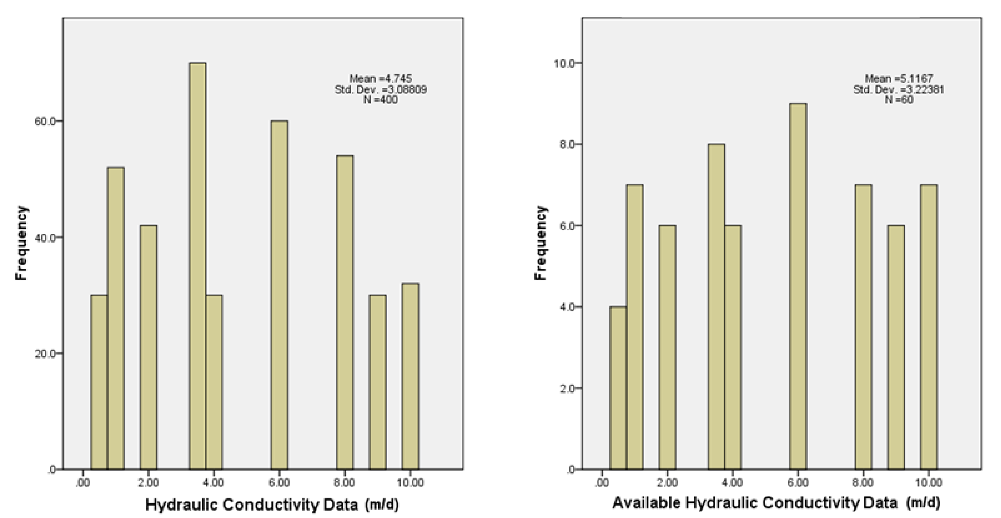
• From geostatistical analyses, obtain the spatial variogram model for the hydraulic conductivity with the available data (in the case study, it is assumed that only 60 of the total 400 hydraulic conductivity data of the model are known), the spatiotemporal variogram model for hydraulic head with the values simulated each 4 months for a 2-year period (2400 values in total), and the cross variograms for each simulation time of the model between the hydraulic conductivity (60 data) and the corresponding hydraulic head data (400 values).
• Derive separately the covariance matrices for the hydraulic conductivity, the spatiotemporal hydraulic head data and the cross covariances between the hydraulic conductivity and the hydraulic head for each time. The covariance values are obtained for all the estimation and sampling nodes.
• Integrate a multivariable covariance matrix that includes the spatial, spatiotemporal and cross covariances (

  Table 4. Structure of the multivariate spatiotemporal covariance matrix.

  Univariate spatial covariance matrix (hydraulic conductivity only)	Cross-covariance matrix (hydraulic conductivity–hydraulic head for time 1)	Cross-covariance matrix (hydraulic conductivity–hydraulic head for time 2)	…	Cross-covariance matrix (hydraulic conductivity–hydraulic head for time NT)
  Cross-covariance matrix (hydraulic head for time 1–hydraulic conductivity)	Space–time covariance matrix (hydraulic head from time 1 to time NT)
  Cross-covariance matrix (hydraulic head for time 2–hydraulic conductivity)
  …
  Cross-covariance matrix (hydraulic head for time NT–hydraulic conductivity)

  ).
• Estimate using the static Kalman filter, the hydraulic conductivity in all the nodes where these data were not available for the geostatistical analyses.

2.3. The Static Kalman Filter

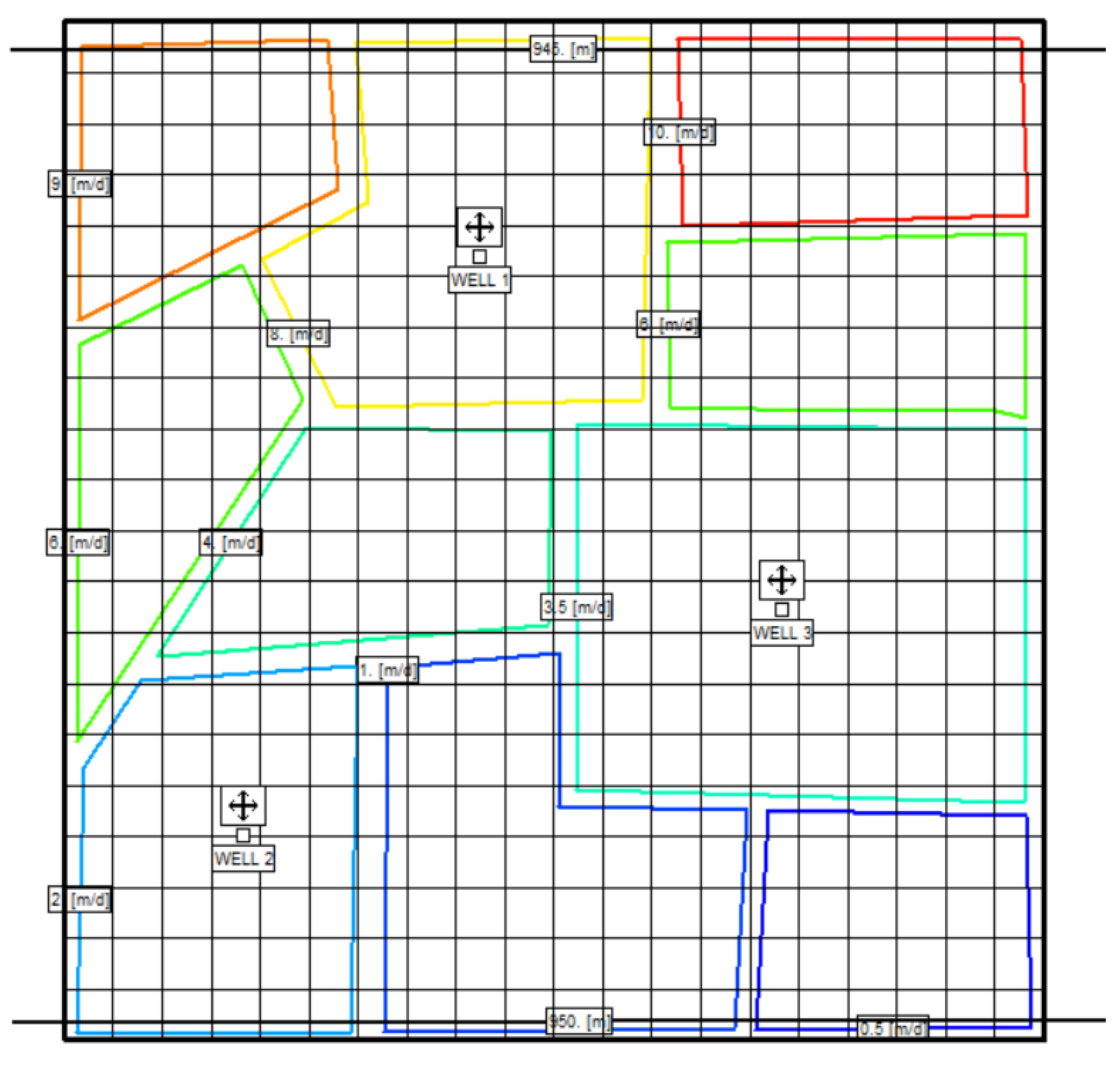
The Kalman filter is a linear, unbiased and optimal estimator for the state of a system at time t, based on available information at time t-1, that estimate is updated with additional available data at time t. The discrete Kalman filter aims to solve the general problem of estimating the state of a discrete-time process, which is represented by a linear stochastic differential equation of the form:

$${\mathrm{X}}_{\mathrm{t}+1}={\mathrm{AX}}_{\mathrm{t}}+{\mathrm{w}}_{\mathrm{t}},$$

(7)

Equation (7) is called the system model, it describes the evolution over time of the quantity to be estimated, expressed by means of a state vector X_t. The transition between states X_t⟶X_t+1 is characterized by the transition matrix A and the addition of a Gaussian white noise vector w_t with covariance matrix Q_t. The vectors and matrices are composed by N and N×N elements, respectively; the same applies for the subsequent cases.

The measurement model relates linearly the measurement vector Z_t to the state of the system X_t through the measurement matrix H and the addition of a Gaussian white noise vector v_t with covariance matrix R_t. Both random variables w_t and v_r are assumed to be independent of each other. The measurement model is as follows:

$${\mathrm{Z}}_{\mathrm{t}}={\mathrm{HX}}_{\mathrm{t}}+{\mathrm{v}}_{\mathrm{t}},$$

(8)

The covariance matrices of the process error Q_t and the measurement error R_t in the most general form of the filter may change over time; however, for simplicity they can be assumed as constants.

The equations for the forecast of the discrete Kalman filter are:

$${\hat{\mathrm{X}}}_{\mathrm{t}+1}^{\mathrm{r}}={\mathrm{A} \hat{\mathrm{X}}}_{\mathrm{t}}^{\mathrm{r}},$$

(9)

$${\mathrm{P}}_{\mathrm{t}+1}^{\mathrm{r}}={\mathrm{AP}}_{\mathrm{t}}^{\mathrm{r}}{\mathrm{A}}^{\mathrm{T}}+{\mathrm{Q}}_{\mathrm{t}},$$

(10)

The equations for correcting the state of the discrete Kalman filter are:

$${\mathrm{K}}_{\mathrm{t}+1}={\mathrm{P}}_{\mathrm{t}+1}^{\mathrm{r}}{\mathrm{H}}^{\mathrm{T}}{\left({\mathrm{HP}}_{\mathrm{t}+1}^{\mathrm{r}}{\mathrm{H}}^{\mathrm{T}}+{\mathrm{R}}_{\mathrm{t}}\right)}^{-1},$$

(11)

$${\hat{\mathrm{X}}}_{\mathrm{t}+1}^{\mathrm{r}+1}={\hat{\mathrm{X}}}_{\mathrm{t}+1}^{\mathrm{r}}+{\mathrm{K}}_{\mathrm{t}+1}\left({\mathrm{Z}}_{\mathrm{t}+1}{\mathrm{H} \hat{\mathrm{X}}}_{\mathrm{t}+1}^{\mathrm{r}}\right),$$

(12)

$${\mathrm{P}}_{\mathrm{t}+1}^{\mathrm{r}+1}=\left(\mathrm{I}-{\mathrm{K}}_{\mathrm{t}+1}\mathrm{H}\right){\mathrm{P}}_{\mathrm{t}+1}^{\mathrm{r}},$$

(13)

where the superscript $\mathrm{r}$ follows the order in which the vectors of the measurements $\{{\mathrm{Z}}_1,{\mathrm{Z}}_2,\dots {\mathrm{Z}}_{\mathrm{N}}\}$ are processed, i.e., $\mathrm{r}=1$ when the measurement ${\mathrm{Z}}_1$ is employed. ${\hat{\mathrm{X}}}_{\mathrm{t}+1}^{\mathrm{r}}$ is the forecast of the state vector at time $\mathrm{t}+1$ using the state vector ${\hat{\mathrm{X}}}_{\mathrm{t}}^{\mathrm{r}}$ at time $\mathrm{t}$, and ${\mathrm{P}}_{\mathrm{t}+1}^{\mathrm{r}}$ is the forecast of the covariance matrix of data at $\mathrm{t}+1$ using the forecast of the covariance matrix of data ${\mathrm{P}}_{\mathrm{t}}^{\mathrm{r}}$ at time $\mathrm{t}$, ${\mathrm{K}}_{\mathrm{t}+1}$ is the Kalman gain and $\mathrm{I}$ is the identity matrix. ${\hat{\mathrm{X}}}_{\mathrm{t}+1}^{\mathrm{r}+1}$ and ${\mathrm{P}}_{\mathrm{t}+1}^{\mathrm{r}+1}$ are, respectively, the corrected state vector and covariance matrix for time $\mathrm{t}+1$, and using $\mathrm{r}+1$ measurements.

For the recursive implementation of these equations, an a priori estimate of the state $\left({\hat{\mathrm{X}}}^{\mathrm{o}}\right)$ and an initial final covariance matrix of the error $\left({\mathrm{P}}^{\mathrm{o}}\right)$ are required. After each update of both time and measurement, the process is repeated taking as a starting point the new estimates of the state and the error covariance [31].

In the way the Kalman filter is implemented in this paper, the state vector does not evolve following a dynamic model, but it is modified by the sampling data (in this case the available hydraulic conductivity and/or hydraulic head data). It is then implemented the static Kalman filter since it employs the measurement and correcting equations only, incorporating time through the use of spatiotemporal vectors [24].

The general form of the measurement vector to be used in this paper for the bivariate spatiotemporal methodology is:

$${\mathrm{Z}}_{\mathrm{t}}={\left[{\mathrm{Z}}_1^1,{\mathrm{Z}}_2^1,\dots ,{\mathrm{Z}}_{\mathrm{NP}1}^1|{\mathrm{Z}}_{1,1}^2,{\mathrm{Z}}_{2,1}^2,\dots ,{\mathrm{Z}}_{\mathrm{NP}2,1}^2|\dots ,\dots ,\dots ,\dots |{\mathrm{Z}}_{1,\mathrm{NT}}^2,{\mathrm{Z}}_{2,\mathrm{NT}}^2,\dots ,{\mathrm{Z}}_{\mathrm{NP}2,\mathrm{NT}}^2\right]}^{\mathrm{T}},$$

(14)

where ${\mathrm{Z}}_{\mathrm{n}}^{\mathrm{m}}$ is the measurement of variable m in position n (it is assumed that this variable does not change through time), ${\mathrm{Z}}_{\mathrm{n},\mathrm{t}}^{\mathrm{m}}$ is the measurement of variable m in position n and time t. The first subvector has a length NP1 that corresponds to the sum of points where the hydraulic conductivity has been sampled (data) and those where it is going to be estimated (unknown data), the others subvectors correspond to the hydraulic head data (all of these have the same length, NP2, equal to the number of data for each of the NT times). The total number of elements of vector ${\mathrm{Z}}_{\mathrm{t}}$ is equal to $\mathrm{N}=\mathrm{NP}1+\mathrm{NP}2\times \mathrm{NT}$, which is also the same number of files and rows of the covariance matrix. In the position for an unknown value, the average value of the elements of the corresponding subvector was used.

In this manner, for the univariate case it is only necessary the first subvector, for the bivariate case the measurement vector should include the first vector and any of the other subvectors (it depends on the selected time to use), and finally, for the multivariate spatiotemporal case it will include the first subvector for the hydraulic conductivity and all the other NT subvectors for the hydraulic head data.

The state vector is built in a similar fashion, but the whole elements for a subvector will be equal to the mean value of the available data for that variable in the corresponding time.

The prior estimate error covariance matrix $\left({\mathrm{P}}^0\right)$ is obtained through geostatistical analyses. In the spatiotemporal geostatistical analysis, a product-sum model is fitted to the sample variogram of pre-existing data (details of the product-sum model can be found in [38,39].

To our knowledge, the implementation of kriging for multivariate spatial-spatiotemporal cases has not been reported; the development of the theory in that sense represents an area of opportunity. In this case, the static Kalman filter is selected as the estimation method since its implementation is simple for the proposed multivariate spatial-spatiotemporal case as is shown in Section 2.2.

2.4. Case Study

The synthetic flow model consists of a confined aquifer in transitory state with a thickness of 500 m that occupies a 5000 m × 5000 m area (2500 hectares) (Figure 1). The storage coefficient has a constant value of 0.15 m³/³, and the hydraulic conductivity ($\mathrm{K}$) values are in the range of 0.2–10 m/day corresponding to clays and sands. The domain was discretized in a block-centered finite difference grid composed by 20 columns and 20 rows (the size of the mesh cells is 250 m × 250 m), so information of hydraulic (hydraulic conductivity and storage coefficient) and hydrogeological (initial conditions) parameters were needed for 400 nodes. The boundary conditions were constant hydraulic head values of 900 m and 950 m at the north and south, respectively, and no-flow boundaries at east and west. Three fully-penetrating pumping wells were included with flow rates of 1000 m³/day each (Figure 1). The initial head was of 1000 m for all the modelled area.

The total simulation period was 2 years; considering 4-month time step, 6 realizations of spatially-distributed hydraulic head data were simulated (400 data for each time).

The groundwater flow equation was solved using the MODFLOW transient flow simulator [42]. The flow equation for an incompressible or slightly compressible fluid in a saturated porous medium can be expressed by combining Darcy’s Law and the continuity equation [43,44]:

$$\nabla ·\left(\mathrm{K}\nabla \mathrm{h}\right)={\mathrm{S}}_{\mathrm{s}}\frac{\partial \mathrm{h}}{\partial \mathrm{t}}+\mathrm{W},$$

(15)

where $\mathrm{K}$ is the hydraulic conductivity ($\mathrm{L}/\mathrm{T}$), $\mathrm{h}$ is the hydraulic head ($\mathrm{L}$); $\mathrm{W}$ represents sources or sinks (${\mathrm{L}}^3/\mathrm{T}$); ${\mathrm{S}}_{\mathrm{s}}$ is the specific storage coefficient (${\mathrm{L}}^{-1}$); $\mathrm{t}$ is the time ($\mathrm{T}$); $\nabla =\left(\partial /\partial \mathrm{x}+\partial /\partial \mathrm{y}+\partial /\partial \mathrm{z}\right)$ is the divergence operator of a vector field and $\nabla ={\left(\partial /\partial \mathrm{x},\partial /\partial \mathrm{y},\partial /\partial \mathrm{z}\right)}^{\mathrm{T}}$ is the gradient operator of a scalar field. The solution of the flow equation is obtained by applying the finite differences numerical method.

It is accepted that relationship between hydraulic conductivity and hydraulic head in the groundwater flow equation is nonlinear (Equation (15)). For this reason, it is not our intention to obtain a final calibration of a numerical flow model with the proposed methodology but the principal aim is to take advantage of hydraulic conductivity (K)—spatiotemporal hydraulic head correlations to reduce estimate error variances of K (even more than for traditional univariate and bivariate estimation) which could be useful to obtain an initial estimate of the hydraulic parameters that reduces the modelling effort, i.e., it is a type of precalibration.

3. Results and Discussion

In the case study, for the bivariate and bivariate spatiotemporal approaches, the Kalman filter is used to assimilate hydraulic head data to improve the estimation of the spatial distribution of hydraulic conductivity. Univariate, bivariate and bivariate spatiotemporal cases are compared.

3.1. Univariate Estimation

In this case, only hydraulic conductivity (K) data were used and only 60 were considered as “available” from 400 in total (Figure 2). The vector of measurements consists of 400 positions (the first subvector for Equation (14)), which includes the 60 “available” hydraulic conductivity data and the average value of these values for the remaining 340 positions. The state vector is of 400 positions with the average value of the 60 “available” hydraulic conductivity data as the initial state. The covariance matrix has 400 rows and 400 columns (structured as shown in Table 1); it is derived using the selected variogram model for 60 “available” hydraulic conductivity data (

Table 5. Parameters of the fitted variogram models.

Case	Variable	Correlation	Nugget (m2)	Sill(m2)	Range (m)
Univariate	K		0 *	6.69 *	2177.608
	H1		0	0.075	1616.284
	H2		0	0.209	4327.53
	H3		0	0.413	4364.75
	H4		0	0.491	4364.75
	H5		0	0.541	4364.75
	H6		0	0.571	4364.75
Bivariate	K-H1	−0.282	0 µ	−0.200 µ	1500
	K-H2	−0.135	0 µ	−0.160 µ	1500
	K-H3	−0.120	0 µ	−0.200 µ	1800
	K-H4	−0.127	0 µ	−0.230 µ	1800
	K-H5	−0.131	0 µ	−0.250 µ	1800
	K-H6	−0.133	0 µ	−0.260 µ	1800
	H1-K	−0.173	0 µ	−0.200 µ	1550
	H2-K	−0.251	0 µ	−0.260 µ	2000
	H3-K	−0.294	0 µ	−0.340 µ	1800
	H4-K	−0.306	0 µ	−0.380 µ	1800
	H5-K	−0.309	0 **	−0.400 µ	1800
	H6-K	−0.326	0 **	−0.430 µ	1800
Spatiotemporal	Space H		0.09	0.41	3000
	Time H		0.14 Ω	0.09 Ω	1.20 β
	Space-time H			0.41 α

Units: * ${\mathrm{m}}^2/{\mathrm{day}}^2$, ^µ ${\mathrm{m}}^2/\mathrm{day}$, ^Ω ${\mathrm{day}}^{-2}$, ^β ${\mathrm{day}}^{-1}$, ^α $\mathrm{m}·\mathrm{day}$; K is the hydraulic conductivity; HN are data for time N; K-HN means cross variogram for K as primary and HN as the secondary variable; HN-K means cross variogram for HN as primary and K as the secondary variable.

).

Figure 3 shows the histograms for all the hydraulic conductivity data and for the “available” data. It is noticeable that for larger values of the available data, the frequency bars are higher with respect to the others when compared to the former histogram. In addition, for the “available” data histogram the most frequent value is 6 m/day, meanwhile a value of 3.5 m/day corresponds to the histogram for all the data. These characteristics of the variograms are reflected in the mean value which is larger for the “available” data.

3.2. Bivariate Estimation

For the bivariate estimation, the hydraulic conductivity (K) is estimated using the 60 “available” hydraulic conductivity data and 400 hydraulic head data for a selected time; in the case study, six different estimates were obtained since hydraulic head data for six different times were available.

The vector of measurements for each of these estimates has the double of positions relative to the univariate case, because it now includes also the 400 positions for the corresponding hydraulic head data. In a similar manner, the state vector is increased in 400 positions but the value for these new positions is the average value for the corresponding hydraulic head data. The cross covariance is constructed for 800 rows and 400 columns as stated in Table 2 and using the parameters of the corresponding parameters shown in Table 5.

3.3. Bivariate Spatiotemporal Estimation

In this case, the estimation of K is carried out by employing the spatiotemporal correlation between the 60 “available” hydraulic conductivity data and 2400 hydraulic head data (400 data for each of the six times), additionally the cross correlation between the hydraulic head data for each time and the hydraulic conductivity are used.

The vector of measurements includes 400 positions for the hydraulic conductivity (it is constructed in the same manner as in the previous cases) and 2400 positions for the hydraulic head data. The state vector is also of 2800 positions (7 subvectors of 400 positions each), the first subvector is the same than the previous cases, each of the other six subvectors correspond to a specific time, its values are the average of hydraulic head of the corresponding time. The covariance matrix is constructed as shown in Table 3, it has 2800 rows and 2800 columns.

The parameters of the variogram models selected to fit the sampling variograms are presented in Table 5. The evaluation for selecting the best fit for all the analysed cases was done through cross validation. All the selected models are spherical. It can be seen that the sill values for the hydraulic conductivity are much larger when they are compared with the hydraulic head; it is noteworthy that the sill values for hydraulic head in years 1 and 2 are very low with respect to the other years, in particular the hydraulic head in year 1 has the lowest sill value by far but also the minimum range of the variogram models.

By using the Pearson correlation coefficient obtained through the adjusted sill values of the cross variogram models, numerical values between −0.120 and −0.326 were found, which indicates that there exists a low negative linear correlation among K and H; nevertheless, the idea of this research work is to take advantage of the existent correlation because somehow it contributes to improving the K estimation.

Cross validation results are presented in

Table 6. Cross validation results for the fitted variogram models.

Case	Variable	Minimum Error (m)	Maximum Error (m)	Mean Error (m)	MSE (m2)	RMSE	SMSE
Univariate	K	−2.171 *	3.063 *	0.0031 *	1.0343 **	1.017 *	0.501
	H1	−0.056	0.256	−0.0002	0.0005	0.022	0.035
	H2	−0.098	0.254	−0.0001	0.0006	0.024	0.028
	H3	−0.149	0.254	−0.0001	0.0007	0.026	0.022
	H4	−0.183	0.264	−0.0001	0.0007	0.027	0.020
	H5	-0.204	0.253	−0.0001	0.0008	0.028	0.019
	H6	−0.217	0.263	−0.0001	0.0008	0.028	0.019
Bivariate	K-H1	−2.146 *	2.608 *	0.0346 *	0.9754 **	0.988 *	0.283
	K-H2	−2.140 *	2.612 *	0.0361 *	0.9738 **	0.987 *	0.282
	K-H3	−2.138 *	2.613 *	0.0366 *	0.9732 **	0.986 *	0.282
	K-H4	−2.138 *	2.615 *	0.0368 *	0.9729 **	0.986 *	0.282
	K-H5	−2.137 *	2.615 *	0.0370 *	0.9728 **	0.986 *	0.282
	K-H6	−2.137 *	2.616 *	0.0370 *	0.9729 **	0.986 *	0.282
	H1-K	−0.056	0.260	−0.0002	0.0005	0.023	0.167
	H2-K	−0.093	0.255	−0.0003	0.0006	0.025	0.080
	H3-K	−0.142	0.256	−0.0004	0.0007	0.027	0.063
	H4-K	−0.175	0.265	−0.0005	0.0008	0.029	0.058
	H5-K	−0.195	0.255	−0.0005	0.0009	0.029	0.054
	H6-K	−0.208	0.265	−0.0006	0.0009	0.030	0.054
Spatiotemporal	Space-time H	−0.366	0.351	−0.0018	0.0047	0.069	0.023

Units: * $\mathrm{m}/\mathrm{day}$, ** ${\mathrm{m}}^2/{\mathrm{day}}^2$.

. The minimum, maximum and mean errors for all cases are small, considering the high variability of data employed in the analysis, the mean square error (MSE) and the root mean square error (RMSE) are acceptable; however, the standardized mean square error (SMSE) is low in all the cases, indicating that the estimated variance is overestimated.

Lower values of RMSE (lower than 0.03 m/day) were obtained after the cross validation for the bivariate cases considering the scenarios with HN and K as the primary and secondary variables, respectively. These RMSE were similar to the univariate cases using the HN variable. The larger RMSE obtained in the validation was for the univariate case using the K variable, nevertheless it was not significant (~1 m/day); similar results were obtained for the validation of the bivariate case with K-HN scenarios.

In Figure 4, a similar pattern can be seen for the three estimation methods; as expected, the different zones of hydraulic conductivity are not delineated as in the model due to the fact that estimates are weighed values of the “available” data, resulting in intermediate values for hydraulic conductivity estimates. This also explains that the central part is poorly reproduced due to the influence of the contrasting values of the data at the northern and the southern part of the model. The bivariate and bivariate spatiotemporal estimations better reflect the northern part of the model corresponding to the largest values; on the other hand the univariate estimation reflects better the southern part with the smallest values. The bivariate case presented in Figure 4, Figure 5 and Figure 6 corresponds to the use of the “available” hydraulic conductivity data and the first year of hydraulic head data.

The histograms (Figure 5) show that the largest values of frequency for the hydraulic conductivity (K) estimates are lower than those of hydraulic conductivity data of the model, in the former more different values are obtained (intermediate values between the model data); therefore, these new values correspond to new bars in the histogram. Large estimates trend seems to be well represented; however, low values (<4) present higher relative frequencies when compared to the hydraulic conductivity data of the model. All the cases produce the highest frequency for some estimates of low values which do not correspond to original data; bivariate cases reach highest peaks for frequencies of estimates with low values. The mean and standard deviation values for estimates are closer to those corresponding to all the hydraulic conductivity data of the model than to the same statistics of the “available” data employed in the estimation.

Since the original K data are considered to follow a normal distribution, then about 68% of them fall within one standard deviation of the mean, this band was considered as a confidence interval of the estimates. The results of

Table 7. Analysis of K estimates within the confidence interval.

Case	Data within the Confidence Interval	Data above the Confidence Interval	Data below the Confidence Interval	Data out of the Confidence Interval
Univariate	59.25%	23.25%	17.50%	40.75%
Bivariate K–H1	58.25%	23.25%	18.50%	41.75%
Bivariate K–H2	57.50%	23.25%	19.25%	42.50%
Bivariate K–H3	58.50%	23.25%	18.25%	41.50%
Bivariate K–H4	58.50%	23.25%	18.25%	41.50%
Bivariate K–H5	58.50%	23.25%	18.25%	41.50%
Bivariate K–H6	58.50%	23.50%	18.00%	41.50%
Bivariate spatiotemporal	58.50%	22.25%	19.25%	41.50%

show that the percentage of the estimate values within this confidence interval is very similar for all the analysed cases; it can be seen that for the bivariate spatiotemporal case it is obtained the best balance of the number of estimated values above and below the confidence interval, which may be indicative of the robustness of the method. The lowest number of estimates within the confidence interval corresponds to the bivariate case using K and H2.

The estimate errors of the hydraulic conductivity are presented in

Table 8. Estimation errors of K.

Case	Variables	Mean Error (m/day)	MSE (m2/day2)	RMSE (m/day)	SMSE
Univariate	K	0.091	0.691	0.831	0.403
Bivariate	K and H1	0.096	0.909	0.953	0.574
Bivariate	K and H2	0.099	0.722	0.850	0.449
Bivariate	K and H3	0.098	0.720	0.848	0.438
Bivariate	K and H4	0.099	0.722	0.850	0.441
Bivariate	K and H5	0.100	0.724	0.851	0.444
Bivariate	K and H6	0.099	0.724	0.851	0.445
Bivariate spatiotemporal	K, H1, H2, H3, H4, H5 and H6	0.095	0.757	0.870	0.469

. The minimum mean error and MSE (and therefore the RMSE) are obtained for the univariate case. For the three estimation methods, errors are very low; the improvement in the estimates of K by using its spatial or spatiotemporal correlation with a secondary variable (in this case, HH) can be appreciated in the SMSE values (closer to one) which reflects a better agreement between the errors and the estimate error variances.

Furthermore, Figure 6 shows that even though errors in the case study are lower for the univariate case, a reduction in estimation uncertainty (expressed with the estimate error variance) is gained for the bivariate cases. In particular, the bivariate spatiotemporal case reduces the most this uncertainty. There is a general trend of a higher estimate uncertainty at the southern region of the model, corresponding to the smallest values of hydraulic conductivity. The values of the SMSE for the bivariate cases (closer to one) along with their respective lower estimate error variances validate a bigger robustness and confidence for these estimation methods when compared to the univariate case; in other words, a lower overestimation of the estimate error variance is reached. In this sense, with respect to these measurements, the best results are obtained for the bivariate spatiotemporal case.

Another comparison of errors in hydraulic heads obtained with the numerical flow model was obtained, the error being the difference between the simulated hydraulic head for the spatial distribution of the 400 known K data (original model) and those hydraulic head values simulated for the different spatial arrays of K estimates; the results are very good for all the cases. In

Table 9. Errors of simulated hydraulic head.

Time	Univariate		Bivariate		Bivariate Spatiotemporal
	Mean Error (m)	MSE (m2)	Mean Error (m)	MSE (m2)	Mean Error (m)	MSE (m2)
1	−0.0133	0.0044	−0.0146	0.0031	−0.0192	0.0033
2	−0.0220	0.0072	−0.0248	0.0050	−0.0340	0.0056
3	−0.0290	0.0088	−0.0329	0.0064	−0.0460	0.0077
4	−0.0339	0.0097	−0.0389	0.0073	−0.0554	0.0094
5	−0.0375	0.0103	−0.0434	0.0081	−0.0623	0.0109
6	−0.0398	0.0107	−0.0461	0.0085	−0.0670	0.0120

, it can be seen that the lowest mean errors are obtained for the univariate case; however, the best results for the Mean Squared Error (MSE) correspond to the presented bivariate case (K–H6). According to this comparison, the best results for the bivariate spatiotemporal case are obtained for the first half of the simulation period; this suggests the decrease in the contribution of hydraulic head data to improve the estimation of K when the cross-variance has been significantly reduced.

It is observed in Figure 7 that the spatial configuration of the hydraulic head in Time 6 for the original model is well represented for the different arrays of K; a general overestimation of the hydraulic head is obtained.

4. Conclusions

Knowledge of hydraulic conductivity within an aquifer is crucial for the development of numerical flow models; however, data for this variable are usually scarce. Several methodologies, mostly geostatistics-based, have been developed in order to estimate the hydraulic conductivity at nonsampled sites. It was first addressed the univariate case (using hydraulic conductivity data only) and later bivariate cases which use the correlation with a secondary variable (usually more sampled) to improve the estimation.

Even though the best estimates were obtained for the univariate case (Mean error = 0.091$\mathrm{m}/\mathrm{day}$, MSE = 0.691 ${\mathrm{m}}^2/{\mathrm{day}}^2$ and RMSE = 0.831 $\mathrm{m}/\mathrm{day}$), a better correspondence between estimate errors and estimate error variance correspond to the bivariate cases (SMSE = 0.574 for the bivariate K-H1 case and SMSE = 0.469 for the bivariate spatiotemporal). Furthermore, the lowest estimate error variances were obtained for the bivariate spatiotemporal case. According to confidence intervals, the spatiotemporal case also produced the more balanced option. In addition, when the K estimates are used for modelling purposes, the best MSE values for H are obtained for the K-H6 bivariate spatial case followed closely by the bivariate spatiotemporal case. The proposed spatiotemporal estimation methodology addresses the calibration problem of nonuniqueness relation between hydraulic head and K through the use of the correlation between K and spatiotemporal HH data of the particular case study and conditioning of estimates with the data comprised in the measurement and state vectors of the Kalman filter implementation; the results show that bivariate spatiotemporal estimations have perspectives to reduce the uncertainty in the estimation of poorly sampled variables; however, the effort is large and in some cases it is not justified if a poor correlation between the primary and the secondary variable exists (maximum and minimum of 0.63 and 0.26, respectively).

In this paper, MODFLOW was used only to produce the synthetic data and to test the proposed methodology. In this sense, this proposal is not a model-based methodology but uses geostatistical analyses of available hydrogeological data to make the construction of a model easier. From our perspective, the estimation proposed in this paper has the advantage of conditioning the initial distribution of K not only to those values reported from pumping tests but also simultaneously to the available hydraulic head data, which could reduce the possibility of obtaining a misleading calibration since this process is susceptible to yield nonrealistic hydraulic conductivity spatial distributions.

Further research should consider the implementation of multivariate estimation methods that take into account the nonlinear relationship between hydraulic head and hydraulic conductivity in order to produce better results. This in fact would represent a more refined precalibration effort. Another topic of interest is to evaluate the effect of the distribution and amount of available data to estimate the hydraulic parameters. In addition, an opportunity area for development in these types of methodologies is the inclusion of more hydraulic parameters such as the specific storage or other variables like solute concentrations as it has been developed for model-based calibration methods.

References

1. Cernicchiaro, G.; Barmak, R.; Teixeira, W.G. Digital interface device for field soil hydraulic conductivity measurement. J. Hydrol. 2019, 576, 58–64. [Google Scholar] [CrossRef]
2. Lu, C.; Lu, J.; Zhang, Y.; Hastings-Puckett, M. A convenient method to estimate soil hydraulic conductivity using electrical conductivity and soil compaction degree. J. Hydrol. 2019, 575, 211–220. [Google Scholar] [CrossRef]
3. Won, J.; Park, J.; Choo, H.; Burns, S. Estimation of saturated hydraulic conductivity of coarse-grained soils using particle shape and electrical resistivity. J. Appl. Geophys. 2019, 167, 19–25. [Google Scholar] [CrossRef]
4. Divya, P.V.; Viswanadham, B.V.S.; Gourc, J.P. Hydraulic conductivity behaviour of soil blended with geofiber inclusions. Geotext. Geomembr. 2018, 46, 121–130. [Google Scholar] [CrossRef]
5. Wu, J.; Deng, Y.; Zheng, X.; Cui, Y.; Zhao, Z.; Chen, Y.; Zha, F. Hydraulic conductivity and strength of foamed cement-stabilized marine clay. Constr. Build. Mater. 2019, 222, 688–698. [Google Scholar] [CrossRef]
6. Ziccarelli, M.; Valore, C. Hydraulic conductivity and strength of pervious concrete for deep trench drains. Geomech. Energy Environ. 2019, 18, 41–55. [Google Scholar] [CrossRef]
7. Zhong, R.; Xu, M.; Vieira, N.R.; Wille, K. Influence of pore tortuosity on hydraulic conductivity of pervious concrete: Characterization and modeling. Constr. Build. Mater. 2016, 125, 1158–1168. [Google Scholar] [CrossRef]
8. Turco, M.; Brunetti, G.; Carbone, M.; Piro, P. Modelling the hydraulic behaviour of permeable pavements through a reservoir element model. Hydrology and Water Resources. Int. Multidiscip. Sci. Geoconf SGEM 2018, 18, 507–514. [Google Scholar] [CrossRef]
9. Di Dato, M.; Bellin, A.; Fiori, A. Convergent radial transport in three-dimensional heterogeneous aquifers: The impact of the hydraulic conductivity structure. Adv. Water Resour. 2019, 131. [Google Scholar] [CrossRef]
10. Jarzyna, J.A.; Puskarczyk, E.; Motyka, J. Estimating porosity and hydraulic conductivity for hydrogeology on the basis of reservoir and elastic petrophysical parameters. J. Appl. Geophys. 2019, 167, 11–18. [Google Scholar] [CrossRef]
11. Tang, R.; Zhou, G.; Jiao, W.; Ji, Y. Theoretical model of hydraulic conductivity for frozen saline/non-saline soil based on freezing characteristic curve. Cold Reg. Sci. Technol. 2019, 165, 102794. [Google Scholar] [CrossRef]
12. Luo, W.; Grudzinski, P.B.; Pederson, D. Estimating hydraulic conductivity from drainage patterns—A case study in the Oregon Cascades. Geology 2010, 38, 335–338. [Google Scholar] [CrossRef]
13. Brunetti, G.; Šimůnek, J.; Bogena, H.; Baatz, R.; Huisman, J.A.; Dahlke, H.; Vereecken, H. On the information content of cosmic-ray neutron data in the inverse estimation of soil hydraulic properties. Vadose Zone J. 2019, 18, 180123. [Google Scholar] [CrossRef] [Green Version]
14. Hörning, S.; Sreekanth, J.; Bárdossy, A. Computational efficient inverse groundwater modeling using Random Mixing and Whittaker–Shannon interpolation. Adv. Water Resour. 2019, 123, 109–119. [Google Scholar] [CrossRef]
15. Batlle-Aguilar, J.; Cook, P.G.; Harrington, G.A. Comparison of hydraulic and chemical methods for determining hydraulic conductivity and leakage rates in argillaceous aquitards. J. Hydrol. 2016, 532, 102–121. [Google Scholar] [CrossRef]
16. Kazakis, N.; Vargemezis, G.; Voudouris, K.S. Estimation of hydraulic parameters in a complex porous aquifer system using geoelectrical methods. Sci. Total Environ. 2016, 550, 742–750. [Google Scholar] [CrossRef]
17. Zhang, Y.; Schaap, M.G. Estimation of saturated hydraulic conductivity with pedotransfer functions: A review. J. Hydrol. 2019, 575, 1011–1030. [Google Scholar] [CrossRef]
18. Abdelbaki, A.M. Using automatic calibration method for optimizing the performance of Pedotransfer functions of saturated hydraulic conductivity. Ain Shams Eng. J. 2016, 7, 653–662. [Google Scholar] [CrossRef] [Green Version]
19. Priyanka, B.N.; Mohan-Kumar, M.S.; Amai, M. Estimating anisotropic heterogeneous hydraulic conductivity and dispersivity in a layered coastal aquifer of Dakshina Kannada District, Karnataka. J. Hydrol. 2018, 565, 302–317. [Google Scholar] [CrossRef]
20. Zhou, H.; Gómez-Hernández, J.J.; Hendricks-Franssen, H.J.; Li, L. An approach to handling non-Gaussianity of parameters and state variables in ensemble Kalman filtering. Adv. Water Resour. 2011, 34, 844–864. [Google Scholar] [CrossRef] [Green Version]
21. Lee, S.; Carle, S.F.; Fogg, G.E. Geologic heterogeneity and a comparison of two geostatistical models: Sequential Gaussian and transition probability-based geostatistical simulation. Adv. Water Resour. 2007, 30, 1914–1932. [Google Scholar] [CrossRef]
22. Jazwinski, A.H. Stochastic Processes and Filtering Theory, 1st ed.; Academic Press Elsevier: Amsterdam, The Netherlands, 1970; Volume 64, ISBN 9780080960906. [Google Scholar]
23. Evensen, G. The Ensemble Kalman Filter: Theoreticalformulation and practicalimplementation. Ocean Dyn. 2003, 53, 343–367. [Google Scholar] [CrossRef]
24. van Leeuwen, P.J.; Evensen, G. Data Assimilation and Inverse Methods in Terms of a Probabilistic Formulation. Mon. Weather Rev. 1996, 124, 2898–2913. [Google Scholar] [CrossRef]
25. Herrera, G.S. Cost Effective Groundwater Quality Sampling Network Design. Ph.D. Thesis, University of Vermont, Vermont, VT, USA, 1998. [Google Scholar]
26. Bailey, R.; Baù, D. Ensemble smoother assimilation of hydraulic head and return flow data to estimate hydraulic conductivity distribution. Water Resour. Res. 2010, 46. [Google Scholar] [CrossRef]
27. Burgers, G.; Jan van Leeuwen, P.; Evensen, G. Analysis Scheme in the Ensemble Kalman Filter. Mon. Weather Rev. 1998, 126, 1719–1724. [Google Scholar] [CrossRef]
28. Evensen, G. Data Assimilation-The Ensemble Kalman Filter, 2nd ed.; Springer: Berlin, Germany, 2009. [Google Scholar]
29. Franssen, H.J.H.; Kinzelbach, W. Real-time groundwater flow modeling with the Ensemble Kalman Filter: Joint estimation of states and parameters and the filter inbreeding problem. Water Resour. Res. 2008, 44. [Google Scholar] [CrossRef]
30. Liu, G.; Chen, Y.; Zhang, D. Investigation of flow and transport processes at the MADE site using ensemble Kalman filter. Adv. Water Resour. 2008, 31, 12. [Google Scholar] [CrossRef]
31. Briseño, J.V. Método Para la Calibración de Modelos Estocásticos de Flujo y Transporte en Aguas Subterráneas, Para el Diseño de Redes de Monitoreo de Calidad del Agua. Ph.D. Thesis, Universidad Nacional Autónoma de México, México, 2012. [Google Scholar]
32. Li, L.; Zhou, H.; Gómez-Hernández, J.J.; Hendricks-Franssen, H.J. Jointly mapping hydraulic conductivity and porosity by assimilating concentration data via ensemble Kalman filter. J. Hydrol. 2012, 428–429, 152–169. [Google Scholar] [CrossRef] [Green Version]
33. Xu, T.; Gómez-Hernández, J.J. Probability fields revisited in the context of ensemble Kalman filtering. J. Hydrol. 2015, 531, 40–52. [Google Scholar] [CrossRef] [Green Version]
34. Zovi, F.; Camporese, M.; Hendricks-Franssen, H.J.; Huisman, J.A.; Salandin, P. Identification of high-permeability subsurface structures with multiple point geostatistics and normal score ensemble Kalman filter. J. Hydrol. 2017, 548, 208–224. [Google Scholar] [CrossRef] [Green Version]
35. Xu, T.; Gómez-Hernández, J.J. Simultaneous identification of a contaminant source and hydraulic conductivity via the restart normal-score ensemble Kalman filter. Adv. Water Resour. 2018, 112, 106–123. [Google Scholar] [CrossRef]
36. Deutsch, C.V.; Journel, A.G. GSLIB: Geostatistical Software Library and User’s Guide, 2nd ed.; Oxford University Press: New York, NY, USA, 1997. [Google Scholar]
37. Webster, R.; Oliver, M. Geostatistics for Environmental Scientists, Statistics in Practice, 2nd ed.; John Wiley & Sons: London, UK, 2007; p. 330. [Google Scholar]
38. De Iaco, S.; Myers, D.E.; Posa, D. Space-time analysis using a general product-sum model. Stat. Probab. Lett. 2001, 52, 21–28. [Google Scholar] [CrossRef]
39. De Cesare, L.; Myers, D.; Posa, D. Estimating and modeling space-time correlation structures. Stat. Probab. Lett. 2001, 51, 9–14. [Google Scholar] [CrossRef]
40. Ahmadi, S.H.; Sedghamiz, A. Geostatistical analysis of spatial and temporal variations of groundwater level. Environ. Monit. Assess. 2007, 129, 277–294. [Google Scholar] [CrossRef]
41. Júnez-Ferreira, H.E.; Herrera, G.S. A geostatistical methodology for the optimal design of space–time hydraulic head monitoring networks and its application to the Valle de Querétaro aquifer. Environ. Monit Assess 2013, 185, 3527–3549. [Google Scholar] [CrossRef] [PubMed]
42. Harbaugh, A.W.; Banta, E.R.; Hill, M.C.; McDonald, M.G. MODFLOW-2000, the U.S. geological surveymodular ground-water model—user guide to modularization concepts and the ground-water flow process. Open-File Rep. USA Geol. Surv. 2000, 92, 134. [Google Scholar]
43. Bear, J. Dynamics of Fluids in Porous Media; American Elsevier Pub. Co.: New York, NY, USA, 1972. [Google Scholar]
44. Freeze, R.A.; Cherry, J.A. Groundwater; Englewood Cliffs: Prentice-Hall, NJ, USA, 1979. [Google Scholar]
Figure 1. Hydraulic conductivity spatial configuration and location of pumping wells for the proposed synthetic model.
Water 12 03136 g001
Figure 2. Spatial distribution of hydraulic conductivity data (m/day) for the numerical flow model.
Water 12 03136 g002
Figure 3. Histogram of hydraulic conductivity data (m/day).
Water 12 03136 g003
Figure 4. Estimated hydraulic conductivity (m/day).
Water 12 03136 g004
Figure 5. Histograms of hydraulic conductivity estimates.
Water 12 03136 g005
Figure 6. Hydraulic conductivity estimate error variances.
Water 12 03136 g006
Figure 7. Simulated hydraulic head spatial configurations.
Water 12 03136 g007