Comparison of Terrestrial Water Storage Changes Derived from GRACE/GRACE-FO and Swarm: A Case Study in the Amazon River Basin


1
School of Geodesy and Geomatics, Wuhan University, Wuhan 430079, China
2
School of Architecture and Civil Engineering, Chengdu University, Chengdu 610106, China
3
MOE Key Laboratory of Fundamental Physical Quantities Measurement & Hubei Key Laboratory of Gravitation and Quantum Physics, PGMF and School of Physics, Huazhong University of Science and Technology, Wuhan 430074, China
4
Key Laboratory of Geospace Environment Geodesy, Ministry of Education, Wuhan University, Wuhan 430079, China
5
Nanning Exploration & Survey Geoinformation Institute, Nanning 530022, China
6
Key Laboratory of Earthquake Geodesy, Institute of Seismology, China Earthquake Administration, Wuhan 430071, China
*
Authors to whom correspondence should be addressed.
Water 2020, 12(11), 3128; https://doi.org/10.3390/w12113128
Submission received: 14 September 2020
/
Revised: 5 November 2020
/
Accepted: 6 November 2020
/
Published: 7 November 2020
(This article belongs to the Section Hydrology)
Abstract
:The mass changes in the Earth’s surface internally derived from the Gravity Recovery and Climate Experiment (GRACE) and the GRACE Follow-On (GRACE-FO) missions have played an important role in the research of various geophysical phenomena. However, the one-year data gap between these two missions has broken the continuity of this geophysical research. In order to assess the feasibility of using the Swarm time-variable gravity field (TVGF) to bridge the data gap, we compared Swarm with the GRACE/GRACE-FO models in terms of model accuracy, observation noise and inverted terrestrial water storage change (TWSC). The results of the comparison showed that the difference between the degree-error root mean square (RMS) of the two models is small, within degree 10. The correlation between the spherical harmonic coefficients of the two models is also relatively high, below degree 17. The observation noise values of GRACE/GRACE-FO are smaller than those of Swarm. Therefore, the latter model requires a larger filter radius to lower these noise levels. According to the correlation coefficients and the time series map of TWSC in the Amazon River basin, the results of GRACE and Swarm are similar. In addition, the TWSC signals were further analyzed. The long-term trend changes of TWSC derived from GRACE/GRACE-FO and the International Combination Service for Time-variable Gravity Fields (COST-G)-Swarm over the period from December 2013 to May 2020 were −0.72 and −1.05 cm/year, respectively. The annual amplitudes of two models are 15.65 and 15.39 cm, respectively. The corresponding annual phases are −1.36 and −1.33 rad, respectively. Our results verified that the Swarm TVGF has the potential to extract TWSC signals in the Amazon River basin and can serve as a complement to GRACE/GRACE-FO data for detecting TWSC in local areas.
1. Introduction
The Gravity Recovery and Climate Experiment (GRACE) satellite mission was jointly developed and managed by the National Aeronautics and Space Administration (NASA) in the United States and the Deutsche Zentrum Für Luft- und Raumfahrt (DLR) in Germany. It enabled new observations for estimating mass changes in global or regional areas with the Earth system [1]. GRACE was launched on 17 March 2002 and consisted of two identical satellites, flying in formation, in the same order (an initial altitude of about 520 km). The distance changes between two GRACE satellites were measured by K-band ranging (KBR), which is influenced by global mass changes within the Earth’s interior, at its surface and in the atmosphere. This method is called low–low satellite-to-satellite tracking (ll-SST). The monthly time-variable gravity field (TVGF) solutions were computed according to the pre-processed GRACE along-track KBR data, which are known as the GRACE Level 2 data, in the form of spherical harmonic (SH) coefficients. According to the SH coefficients or mascon solutions, GRACE Level 2 data can be converted to terrestrial water storage change (TWSC) [2,3], polar ice sheet mass variation [4,5], sea level change [6,7], co-seismic gravity change [8,9,10,11], etc. These research efforts have greatly improved our understanding of the whole Earth’s water cycle, cryosphere and internal structure.
The GRACE mission, which ended in June 2017, has continued to provide vast and valuable data [11]. In order to continue the lifetime of GRACE, the GRACE-Follow On (GRACE-FO) mission was launched in May 2018, which began to provide the same TVGF data products since June 2018. The problem is that there is an 11-month data gap between the two satellite missions. Therefore, an alternative and independent data source is needed to fill this gap, aiming to ensure the continuity of related research. In addition to special gravity satellites, low-Earth orbit (LEO) satellites with high quality GPS receivers can also be used for observing the Earth’s gravity field and its long-wavelength temporal variations, in a process known as high–low satellite-to-satellite tracking (hl-SST) [12,13,14,15,16].
The European Space Agency (ESA) successfully launched the Swarm satellites on 22 November 2013. The Swarm mission consists of three identical Earth observation satellites which are all in near-polar orbit, two (Swarm A and Swarm B) at an altitude of about 470 km and one (Swarm C) at an altitude of about 520 km, aiming to study the principle of the Earth’s magnetic field and its changes [17,18]. The three satellites are all equipped with two key instruments for gravity field detection (a high-precision, dual-frequency global navigation satellite system (GNSS) receiver and an accelerometer), which can provide the time series of the Swarm satellite positioning data and non-conservative forces acting on the satellites [19,20]. Because its running time just covers the GRACE/GRACE-FO gap, the Swarm mission has the potential to fill this gap.
Many scientists have studied the potential of LEO satellites to quantify and monitor the Earth’s surface and internal mass changes, such as the Challenging Minisatellite Payload (CHAMP); the Constellation Observing System for Meteorology, Ionosphere and Climate (COSMIC); GRACE and the Gravity Field and Steady-State Ocean Circulation Explorer (GOCE) missions [21,22,23,24,25]. These studies show that hl-SST data from LEO satellites can detect the surface mass changes to various degrees, but compared with the results of GRACE, the noise is greater and the spatial resolution is lower. Wang and Chao [26] used Swarm simulated data to calculate ice sheet mass changes in Greenland. The results showed that Swarm data are suitable for detecting long-wavelength signals and their inversion accuracy can reach 20% of that of GRACE data. The calculation results from Swarm simulated data have proven that Swarm has the potential to recover annual signals up to SH degree 6 [27]. Bezděk et al. [28,29] inferred the Swarm TVGF based on the acceleration approach with a spatial resolution larger than 2000 km, which is a similar quality to GRACE’s GPS-based TVGF. Beutle et al. [30] introduced the principle of using GPS positioning data and accelerometer data from LEO satellites to determine the Earth’s gravity field based on the celestial mechanics approach (CMA). Jäggi et al. [31] applied this method to Swarm satellites and proposed that the Swarm mission is well suited for bridging the gap between GRACE and the GRACE-FO mission. Ilk et al. [32] employed the short-arc method to determine the Swarm TVG field from GNSS positioning data. Weigelt et al. [33] used the refined data processing strategy to derive the Greenland ice sheet mass changes, using hl-SST data. Lück et al. [34] used Swarm and GRACE TVG data to study sea water mass changes, and the long-term trend changes derived from Swarm and GRACE are 3.3 and 3.5 mm year−1, respectively. This suggests that Swarm TVG data have the potential to invert the large-scale Earth surface mass changes. The SH coefficients of TVGF derived from hl-SST data are up to a degree and order from ~10 to 15, and the corresponding spatial resolution is from ~1300 to 2000 km, which shows a big difference compared with that of GRACE (~350 km) [35]. Da Encarnação et al. [36,37] found that the maximum spatial resolution of the Swarm TVGF model is a degree of 12. However, most studies focus on the comparison of the numerical values of long-term trend changes derived from GRACE and Swarm. However, there are few studies on the comparison between the spatial distribution of long-term trend changes and the seasonal changes derived from GRACE and Swarm.
In this study, we focused on the potential of Swarm TVGF to detect TWSC in the Amazon River basin. The results of Swarm are compared with that of GRACE/GRACE-FO. In addition to comparing the two traditional indicators (internal and external coincidence accuracy and long-term trend change), comparisons of the spatial distribution of long-term trend changes, annual change, filter algorithm and correlation coefficient were also carried out in this study. The main contents of this paper are as follows. Section 2 presents an overview of our research areas. Section 3 describes the datasets and data processing methods. Section 4 shows the results, and Section 5 presents the discussion of these findings. Finally, the conclusions are presented in Section 6.
2. Study Area
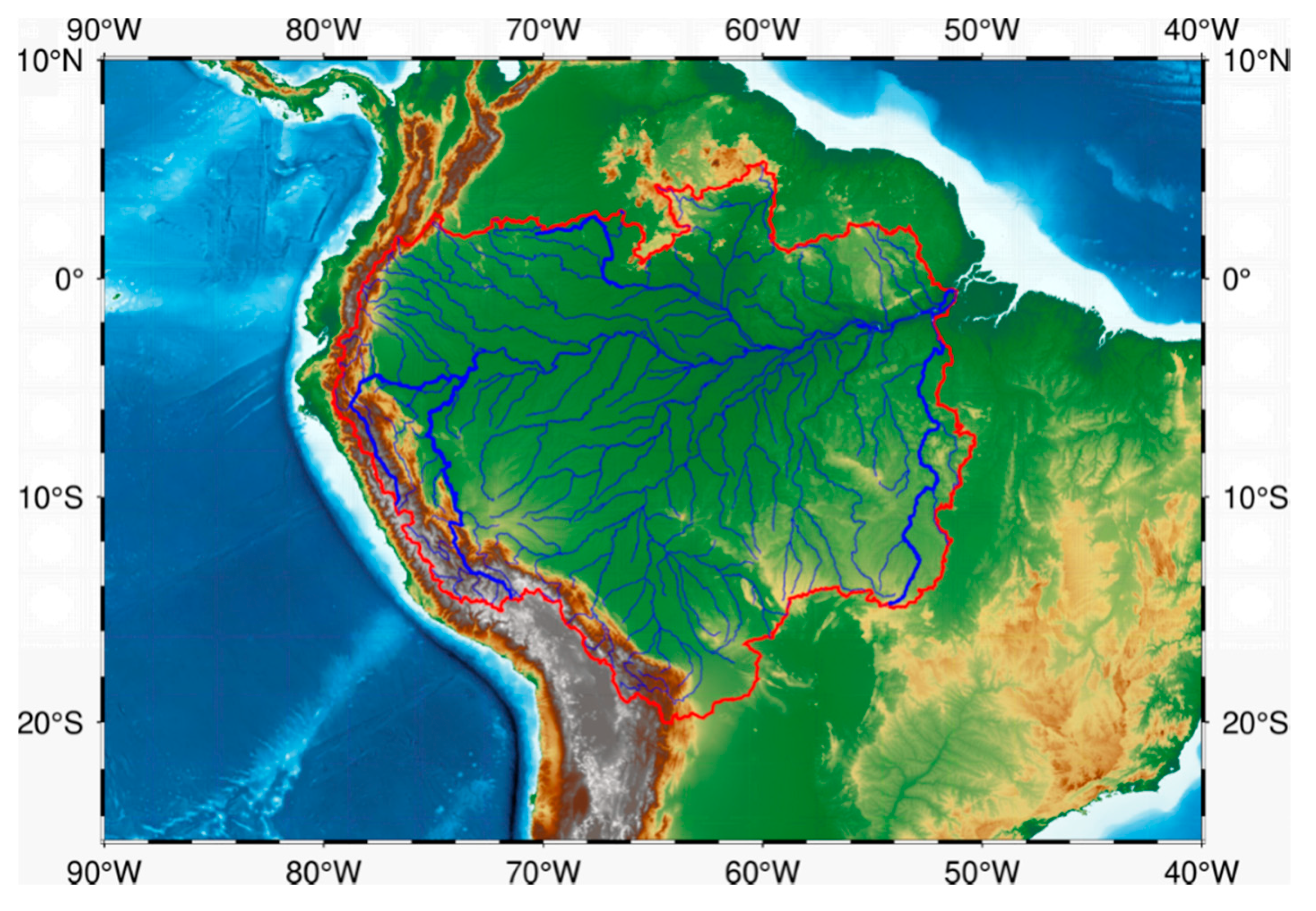
The Amazon River basin, located in the northern part of South America at approximately 5° N–20° S and 50° W–70° W, is the largest river in the world, with the largest discharge, the largest drainage basin and the largest tributaries, as shown in Figure 1. It also has 20% of the world’s river flow. The basin covers an area of 6.915 million square kilometers, accounting for approximately 40% of South America’s total area. Moreover, it is one of the most hydrologically and ecologically diverse regions in the world [38,39]. It has the world’s largest tropical rainforest and 25% of all terrestrial species on Earth live in this area [40]. Therefore, the Amazon River Basin is an important component of global terrestrial ecosystems and the hydrologic cycle [41]. It plays a major role in global atmospheric circulation and affects the global climate change. Therefore, scientists around the world have been studying the water cycle in this area [42].
3. Data and Methodologies
3.1. GRACE/GRACE-FO Data
The GRACE and GRACE-FO monthly SH solutions (truncated to a degree and order 60) used in our study were provided by the Center for Space Research (CSR), University of Texas at Austin, consisting of the GRACE RL06 SH solutions covering the period April 2002 to June 2017 (ftp://isdcftp.gfz-potsdam.de/grace/Level-2/CSR/RL06/) and the GRACE-FO RL06 SH solutions from June 2018 to March 2020 (http://icgem.gfz-potsdam.de/series/01_GRACE/CSR/CSR%20Release%2006%20(GFO)). Before using the above data to invert TWSC, they needed to be preprocessed [43]. Firstly, the C20 term was replaced by the corresponding data from Satellite laser ranging (SLR) because of the lower accuracy of the GRACE TVG model [14]. Secondly, the 1-degree errors of the TVG model caused by geocenter motion were corrected by using the results from Swenson et al. [6]. Thirdly, the effect of ice rebound was deducted from the TVGF model using the ICE-5G glacier isostatic adjustment (GIA) model. Finally, smooth-filtering processing using a 300 km fan filter [2] was used to reduce the observation noise of the GRACE data.
Because GRACE-FO spacecraft and instruments are based on the original design of GRACE and the solution models and methods of GRACE-FO RL06 data are the same as those of GRACE RL06 data, we simply regard GRACE data and GRACE-FO data as GRACE data in order to simplify the comparison in the following research in this paper [1,37].
3.2. Swarm Data
Swarm TVGF data with different solutions were, respectively, provided by the Astronomical Institute at the University of Bern (AIUB), the Astronomical Institute at the Czech Academy of Sciences (ASU), the Institute of Geodesy at Graz University of Technology (IfG) and the International Combination Service for Time-variable Gravity (COST-G). The details of data processing are described in Table 1 [34,37].
It is important to note that the Swarm TVGF models of COST-G were produced by combining the individual Swarm TVGF models from AIUB, ASU, IfG and Ohio State University (OSU) according to the weights defined by variance component estimation (VCE) [37,44]. At present, ASU and COST-G have continued updating data in their website, but the Swarm data have been provided by AIUB and IfG until December 2016. Before inversion processing, the Swarm TVG data must be post-processed, similarly to the GRACE data (the C20 term was replaced by the corresponding data from SLR, the 1-degree errors of the TVG model were corrected and the effect of ice rebound was deducted by using the ICE-5G GIA model).
3.3. Scale Factor Estimated from GLDAS
The Global Land Data Assimilation system (GLDAS), jointly administered by the Goddard Space Flight Center (GSFC) at NASA and the National Centers for Environmental Prediction (NCEP) at the National Oceanic and Atmospheric Administration (NOAA), is a global, high-resolution terrestrial modeling system that incorporates satellite and ground-based observational data products, using advanced land surface modeling and data assimilation techniques [45].
In this study, due to the truncation error and the filtering process, there is a leakage error in the TWSC results. Therefore, this error needs to be corrected. GLDAS monthly gridded data with 1° × 1° for the period of April 2002 to May 2020 were used to assess the scale factors of GRACE and Swarm in the Amazon River Basin. The data processing was carried out as follows [46]:
- (1)
- The time series of regional TWSC was calculated based on global GLDAS original gridded data;
- (2)
- An SH expansion of the original gridded data was performed and truncated to the same degree as the GRACE or Swarm models. These were processed by the same filtering method;
- (3)
- According to the processed SH coefficients, the TWSC time series was computed in regional areas;
- (4)
- The scale factor was calculated according to the time series obtained in step 3 and the original ones using the least squares rule.
3.4. Data Analysis
In order to test the quality of Swarm data, its results were compared with those of GRACE data in terms of model precision, filtering results, time series changes, long-term trend changes and seasonal changes of TWSC in the Amazon River basin.
3.4.1. Degree-Error RMS
In addition to the SH coefficients in the monthly gravity field data file, there are also error estimates. Therefore, the error estimates were used to calculate the corresponding degree-error root mean square (RMS) to evaluate the model’s accuracy in terms of the individual monthly gravity field. In this study, degree-error RMS was used to assess the internal coincidence accuracy of the TVGF model. The calculation formula is as follows [47]:
where and are the SH coefficients errors, and are the degree and order of the SH coefficients and is degree-error RMS, which can also be used to test the internal coincidence accuracy of the monthly gravity field model.
Similarly, the external coincidence accuracy can also be estimated by using the degree-error RMS, and a state-of-the-art static gravity field should be introduced as the reference field. The expression is as follows [11]:
where and are the SH coefficients of the monthly gravity field model, and are the SH coefficients of the reference field and is degree-error RMS when external coincidence accuracy is computed. In this study, ITG-Grace2018s was chosen as the reference field, which is up to degree and order 200, and was provided by the Institute of Geodesy and Geoinformation of Universität Bonn (ITG).
3.4.2. Degree Correlation Analysis
For two different gravity field models, A and B, the correlation coefficient of each degree of the two models can be expressed as [36]:
where are the SH coefficient variance relative to the reference field of monthly gravity field models A and B, respectively, and is the correlation coefficient of each degree of the two models. The correlation analysis of was also carried out according to the above formula.
3.4.3. The Analysis of TWSC Time Series
The TWSC in the Amazon River basin has significant seasonal signals. In order to analyze the potential of TWSC inversion using Swarm TVG data, the TWSC time series inverted by GRACE and Swarm data were decomposed into the long-term trend and seasonal change signals. The decomposition is expressed as follows [48]:
where is the time series of TWSC; is the time; is the error and other signal; and , , , , and are the unknown parameters. is constant term, is long-term trend, and are annual terms and and are semi-annual terms. The amplitude and phase of annual and semi-annual terms are , , and , respectively, of which the expressions are as follows:
4. Results
4.1. Precision Evaluation of the Gravity Filed Model
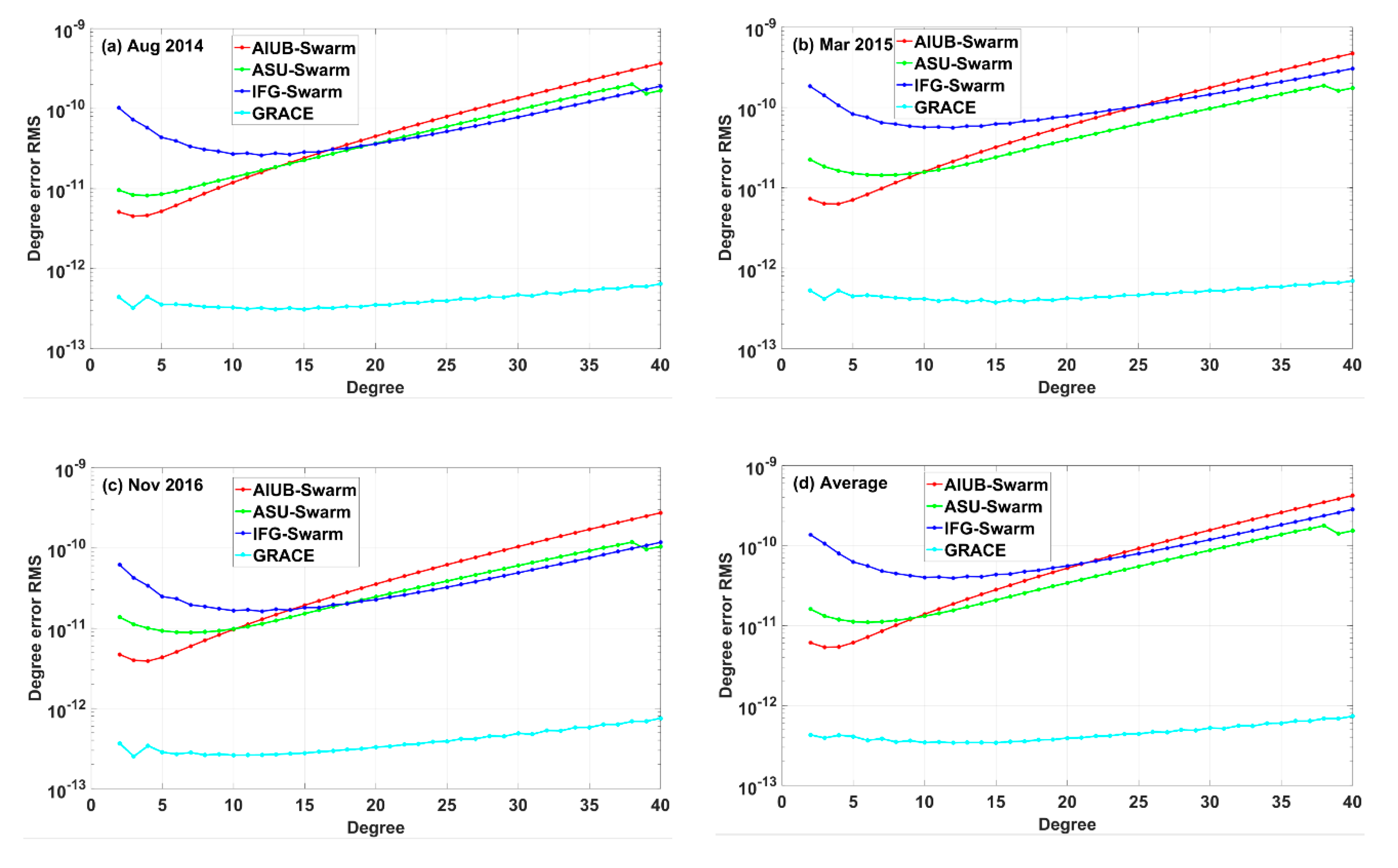
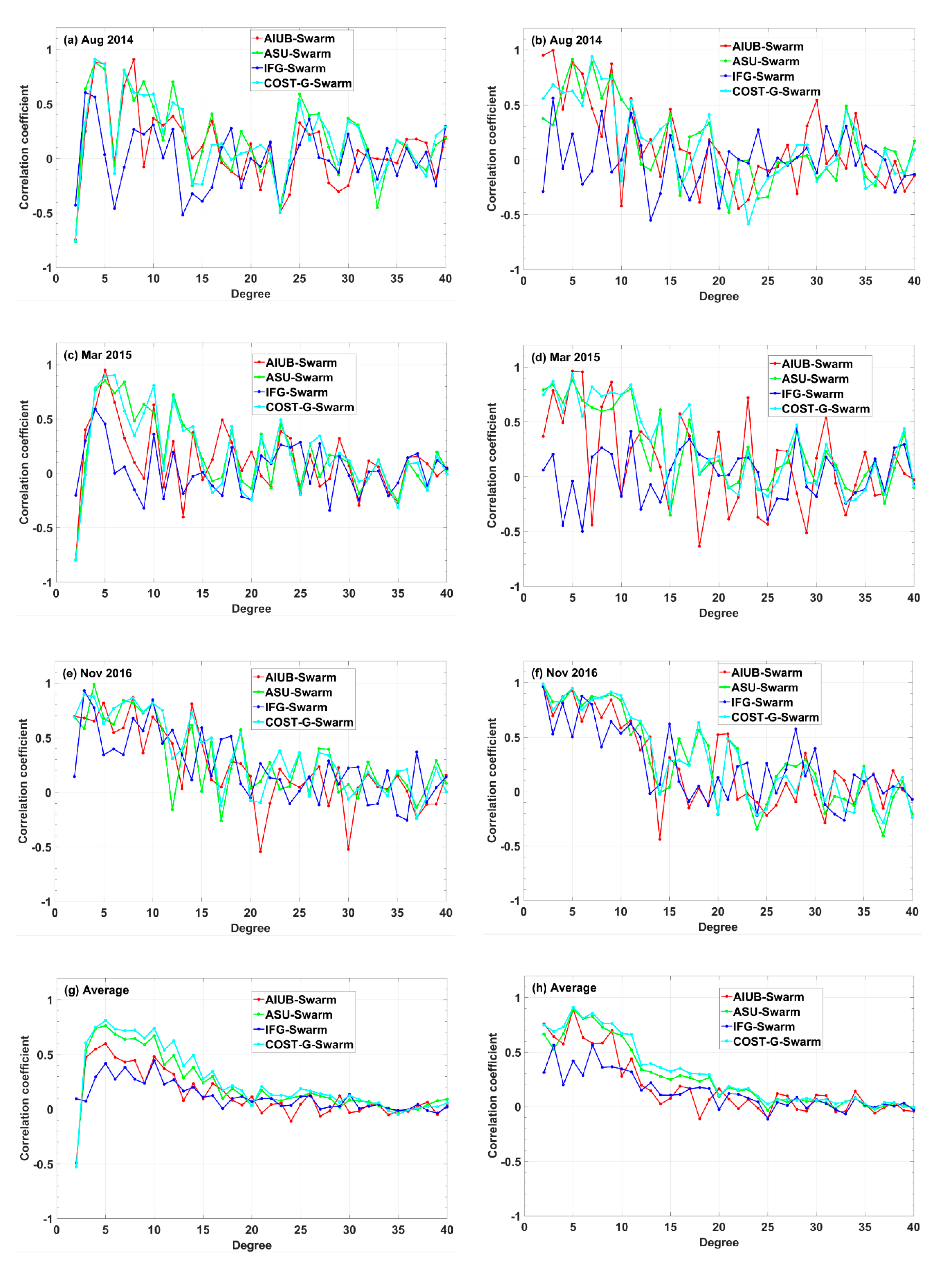
The individual Swarm monthly gravity field solutions were provided by AIUB, ASU, IfG and COST-G. The internal coincidence accuracy of the Swarm and GRACE TVGF models is shown in Figure 2. Although the results of all the months were calculated in this study, the results of three months (August 2014, March 2015, November 2016) are displayed (Figure 2a–c). The average of the results of all the months is displayed in Figure 2d. As can be seen from these Figures, the results are roughly equivalent. According to the comparison, the precision of all models improves with degree increasing, within degree 10. Beyond degree 10, the exact opposite is observed. The model precision of GRACE is about 10 times larger than that of Swarm. The accuracy of the GRACE model is relatively stable and does not appear to exhibit great fluctuations with the increasing degree. Under degree 10, the model precision of AIUB-Swarm is overly optimistic [36]. However, after degree 10, the precision of the AIUB model rapidly decreases with the increasing degree. However, the ASU-Swarm model occupied the optimal position of the three Swarm models, except in Figure 2c. Unfortunately, due to the lack of SH coefficient errors for the COST-G Swarm TVGF model, its degree-error RMS is not presented in these figures.
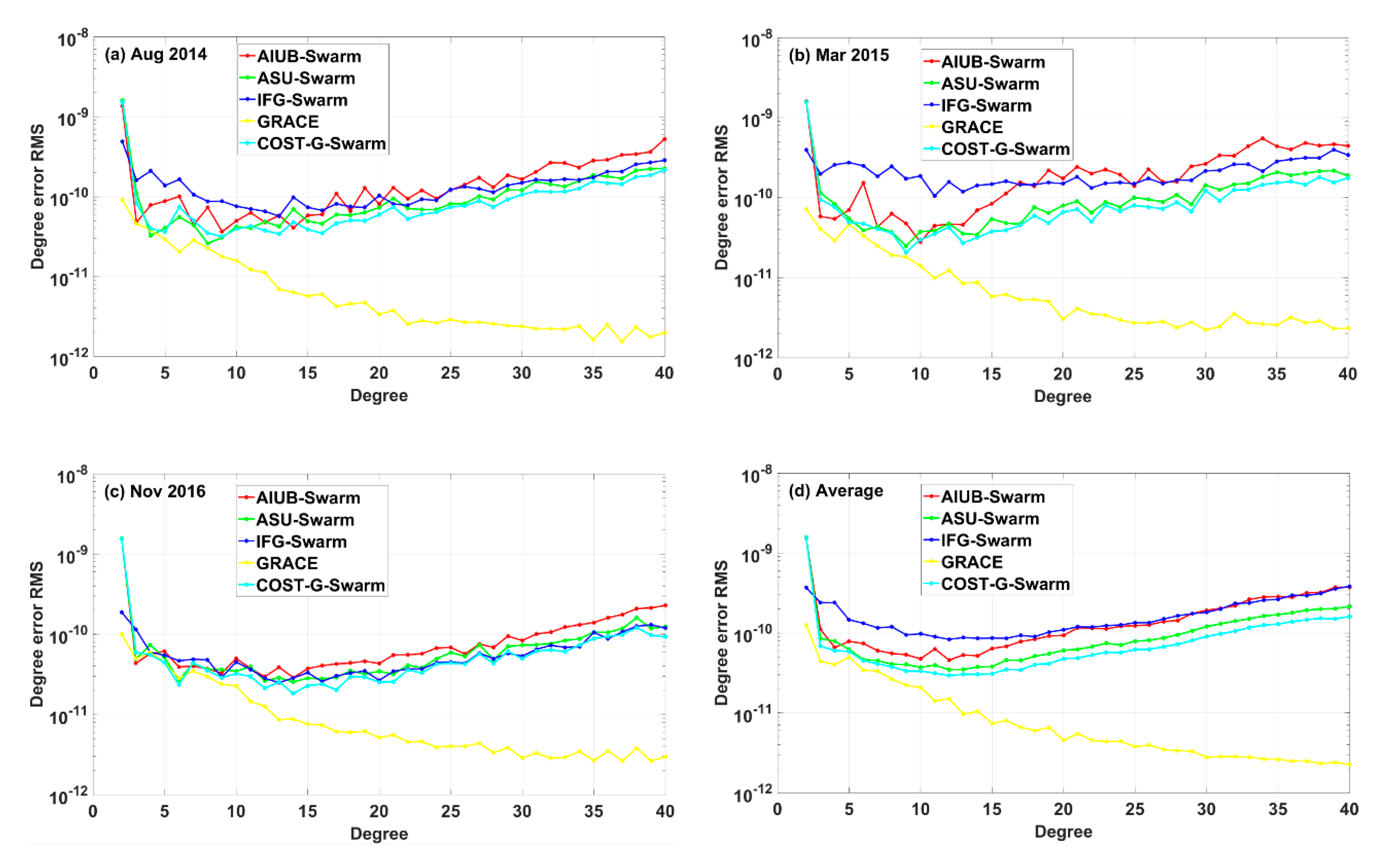
To further compare the model accuracy of Swarm and GRACE, the same reference field (ITG-Grace2018s) was deducted from GRACE and Swarm models for all the months, respectively, in order to obtain the external coincidence accuracy (Figure 3). Figure 3a–c show the results of three random months and the average of all the months is shown in Figure 3d.
According to Figure 3, the accuracy of all the Swarm models is comparable to that of GRACE below degree 10. With this degree range, the amplitude of all the degree-error RMS increases slightly with increasing degree. After degree 10, the precision of the GRACE model improves with increasing degree. The model accuracy of the Swarm models clearly decreases above degree 15. This suggest that noise begins to dominate [36]. Therefore, when the Swarm model is used to detect time-variable signals, it is generally truncated to about degree 15 [35,37]. The model accuracy of COST-G-Swarm is greater than that of other Swarm models. The COST-G-Swarm model, combining different Swarm products from AIUB, ASU, IfG and the Ohio State University (OSU) using the VCE method, has the advantages of various models. In terms of single models, the model precision of ASU-Swarm is greater than that of the others, and is close to that of COST-G-Swarm, as shown in Figure 3d. In general, the accuracy of GRACE model is significantly greater than that of Swarm models.
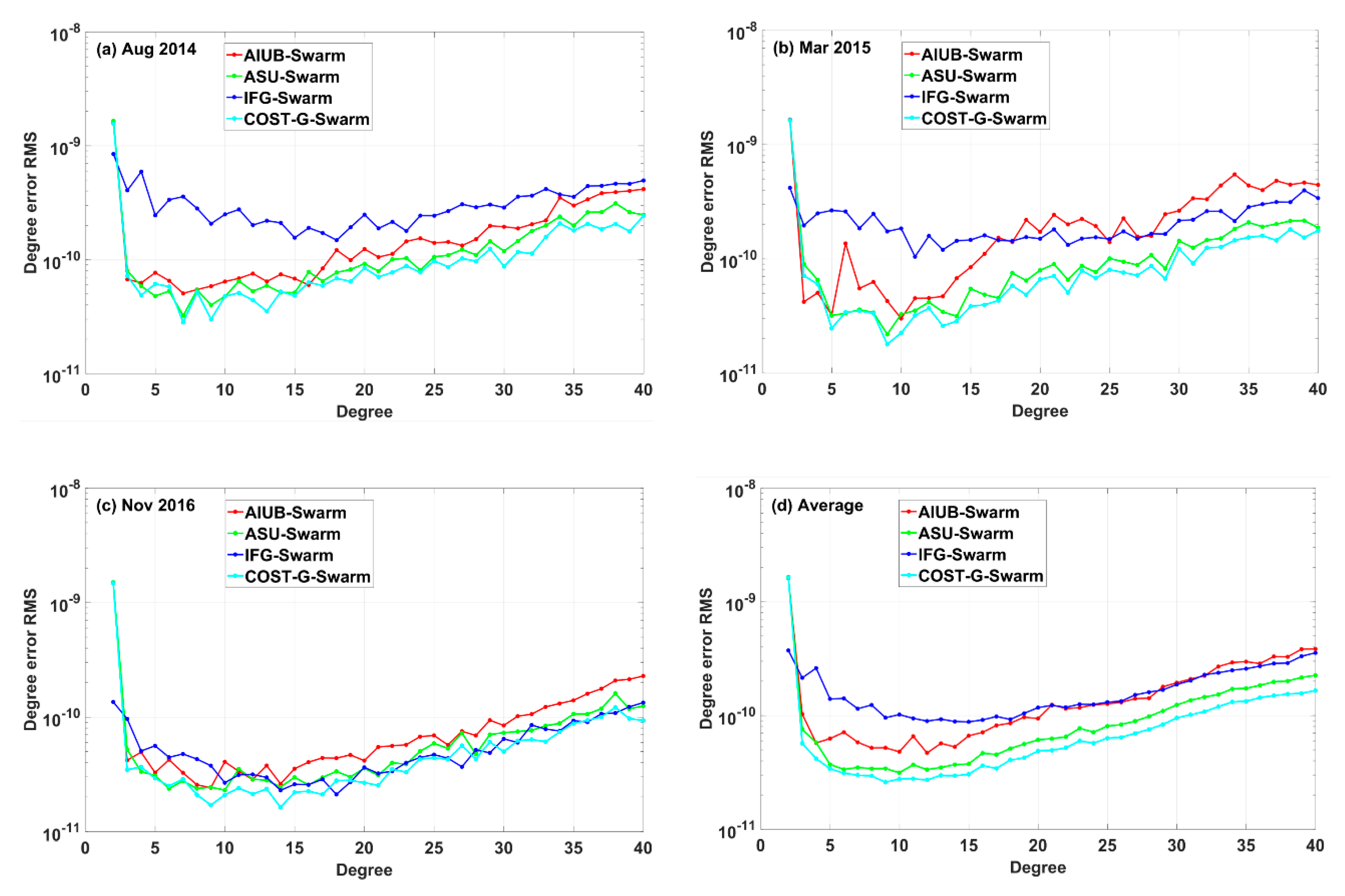
The differences between the SH coefficients from the GRACE and Swarm models were used to calculate the corresponding degree-error RMS (Figure 4). Similarly, the results of three random months and the average results of all the months are shown in these Figures. The same conclusion can be drawn as in Figure 3—that the results of COST-G-Swarm were better than any single model. Of the three single models, the ASU-Swarm model was optimal and closer to the COST-G-Swarm model, except in Figure 4c. Except for the large difference in AIUB-Swarm, the results of the other three models were relatively close, as shown in Figure 4c. Comparing Figure 3 and Figure 4, the degree-error RMS of the residual of the Swarm models relative to the GRACE model is lower than that of the time-variable signals of the Swarm and GRACE models. This means that Swarm TVGF models still reveal the temporal variance of Earth’s gravity field under a limited spatial resolution [36].
In order to determine the maximum degree of Swarm models used for extracting time-variable signals, the degree correlation coefficients between the GRACE and Swarm models are introduced in this paper (Figure 5). These degree correlation coefficients can reflect the number of time-variable signals in the Swarm models relative to the GRACE model, and the degree range of these signals [37]. In Figure 5a, it can be seen that below degree 13 the degree correlation coefficients of all the Swarm models are positive values, in addition to the IfG-Swarm and AIUB-Swarm models. After degree 13, the values fluctuate around 0. However, this degree has different values in different maps. The value of Figure 5c is 15 and that of Figure 5e is 16. The above results are the C coefficient. The results of the S coefficient are not much different. For Figure 5b the value is 15, for Figure 5d it is 14 and for Figure 5f it is 20. Figure 5g,h show the average results of all the months from the Swarm and GRACE models. According the results depicted in these two Figures, the degree correlation coefficient continues to decrease from degree 5, and when it reaches degree 17, the degree correlation coefficient decreases to a lower value and remains stable up to degree 40. These results are similar to the conclusions of Encarnação et al. [36].
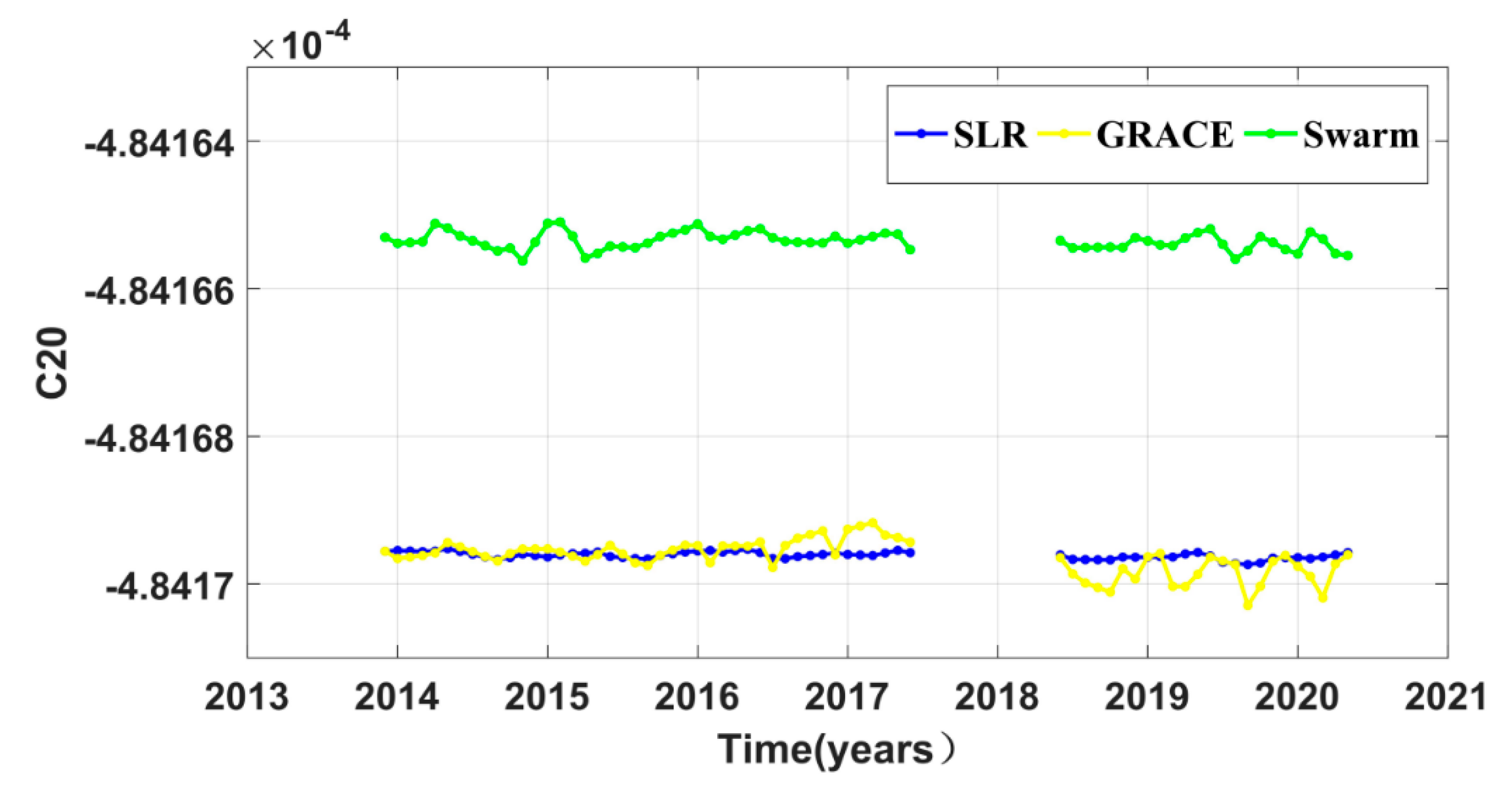
The C20 coefficient is a negative value, due to its lower precision in Swarm models [14] (Figure 6). As seen in Figure 6, there is a big difference between the C20 coefficients from Swarm, GRACE and SLR. However, the C20 coefficients from GRACE and SLR are close. This explains why the correlation coefficient of the C20 term is negative in Figure 5.
According to analysis results of Figure 2 and Figure 3, the precision of Swarm models is worse than that of the GRACE model. The degree-error RMS of Swarm models decreases beyond degree 15, and the correlation coefficients of SH coefficients between GRACE and Swarm models are always positive within degree 17. So, the geophysical signals of Swarm models may be mainly concentrated within degree 17, and the corresponding spatial resolution is about 1200 km. Beyond degree 17, time-variable signals derived from Swarm gravity field models may be mainly noise. Therefore, it is recommended that the SH coefficients should be truncated to degree 17 when Swarm models are used to study TWSC. The low-degree SH coefficients correspond to the long-wave signals part of the gravity field. The Swarm can detect the time-variable signals with a spatial resolution of 1200 km. Furthermore, COST-G-Swarm models are more efficient than single models. Therefore, we used the COST-G-Swarm (referred to as Swarm) model to represent the Swarm model for subsequent research in this paper.
4.2. Filter Results
Due to the orbit error of the satellites, instrument error and imperfections of the gravity field model, the global equivalent water height (EWH), computed using the SH coefficients method, is seriously affected by these noise levels [49]. The noise mainly appears in the high degree part of TVGF, and shows observation noise with north–south distribution features. The spatial smoothing filter method is usually used to reduce the influence of noise, such as the Gaussian filter and fan filter. Since the effect of the fan filter is greater than that of the Gaussian filter, the fan filter was used for processing the noise [50].
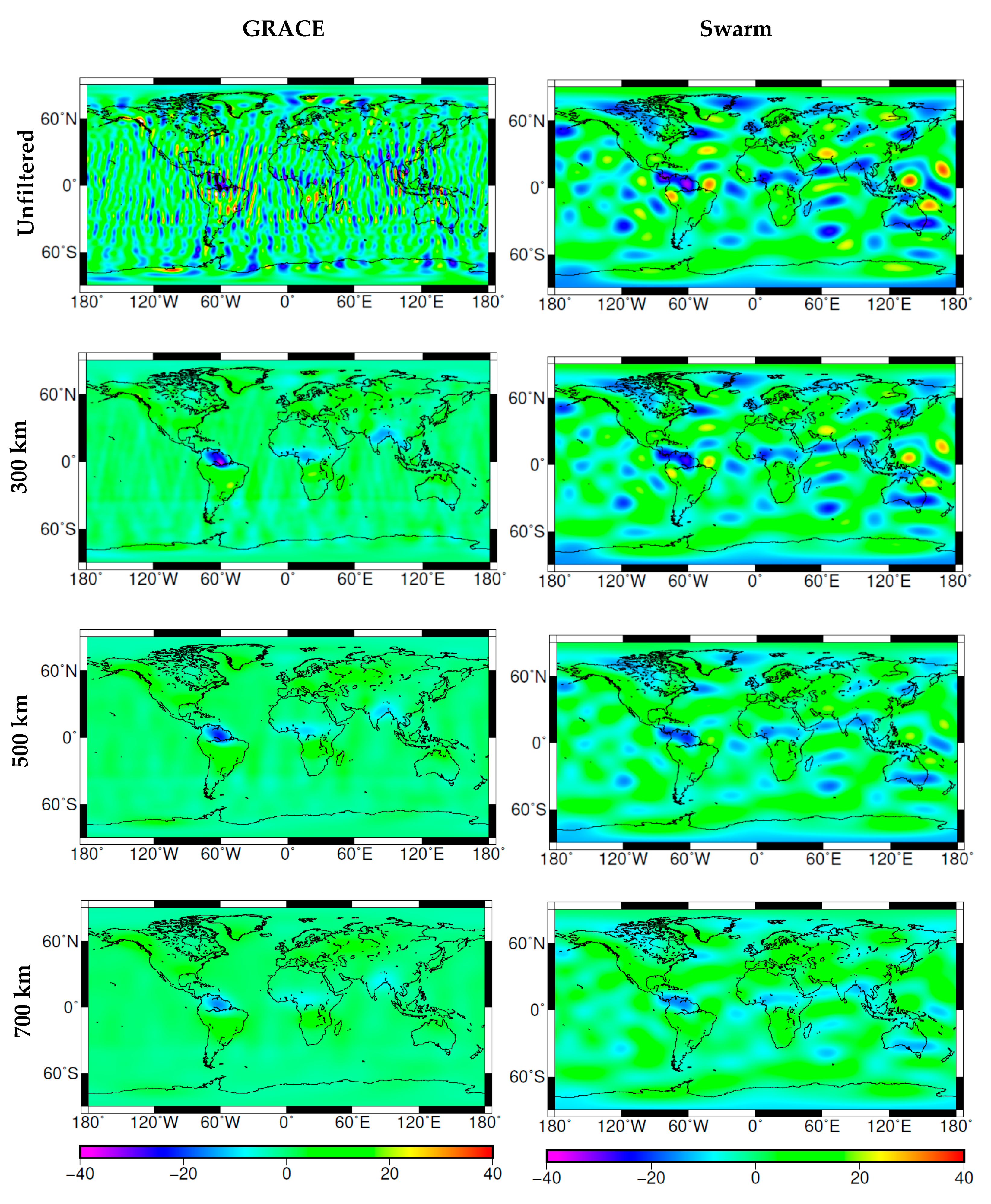
Figure 7 show the filtering results for the GRACE and Swarm models. Before the filtering process, the Swarm model was truncated to degree 17. From unfiltered results, the inversion results of GRACE presented a significant north–south striping effect, and many spots appeared in the Swarm results, most of which were of a negative value. Under the influence of this noise, it is almost impossible to obtain the real signal. Thus, a filtering process is necessary.
When a filter radius of 300 km was applied, the filter effects of GRACE were significantly greater than those of Swarm. The noise affecting the GRACE model was basically eliminated, whereas the noise affecting the Swarm model was partially weakened. When the filter radius was increased to 500 km, it can be seen that part of the real signals in the results of GRACE were filtered. Although the noise in the Swarm model was significantly weakened, there was still a lot of noise. When the filter radius was set at 700 km, the noise in the Swarm model was basically suppressed. Real signals from GRACE were obviously suppressed, such as the Amazon, the Congo and the Ganges rivers. These real signals are dominated by negative values, and positive signals are almost eliminated, compared with the results of the 300 km fan filtering of GRACE. This indicates that the selection of an appropriate filter radius must maintain a balance between reducing the noise signal and keeping the real signal as much as possible.
According to the global EWH distribution of Swarm and GRACE, the results of the two models were the same in some areas with stronger signals—for example, the Amazon, the Congo and the Ganges rivers. However, in other areas, the results of GRACE were different from Swarm, such as in Greenland, the Antarctic, North America and Northeast Asia. As a result, the real signal from GRACE was reduced by the filter with the larger radius, and there was still an influence of residual noise in the Swarm model. We can see a lot of residual noise in the ocean areas in Swarm results.
4.3. TWSC of Amazon River Basin
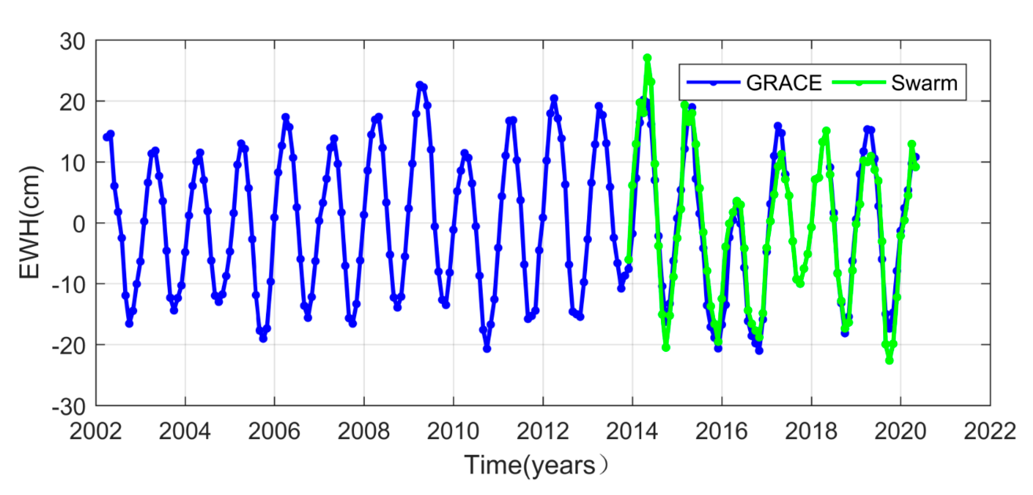
In this section, taking the Amazon River basin as an example, the accuracy of the TWSC derived from Swarm model is discussed. Before inverted TWSC, Swarm SH coefficients with 700 km fan filter processing were truncated to a degree and order of 17, and GRACE SH coefficients were truncated to a degree and order of 60 and were processed using a 300 km fan filter. At the same time, considering the influence of the leakage error, the scale factor method was used to repair the signals. According to the calculation results, the scale factors of the GRACE and Swarm models were 1.05 and 1.23, respectively. It can be seen that the leakage error of Swarm is larger. From Figure 8, the two TWSC time series of the Swarm (green line) and GRACE (blue line) models show significant seasonal variation and the same change trend. However, the amplitude of Swarm is larger than that of GRACE. It can be seen that there were abnormally low values in 2005, 2010, 2015, 2017 and 2019, which is consistent with the fact that drought happened at these points in time [51,52,53]. In addition, significant increases can be observed in 2009, 2010, 2012 and 2014, which are due to flood events [54,55]. According to the comparison of the results of long-term trend change and seasonal signal of TWSC in the Amazon River basin (Table 2), the annual amplitude and annual phase of the Swarm and GRACE models were close. However, their measurements of long-term trend changes were very different.
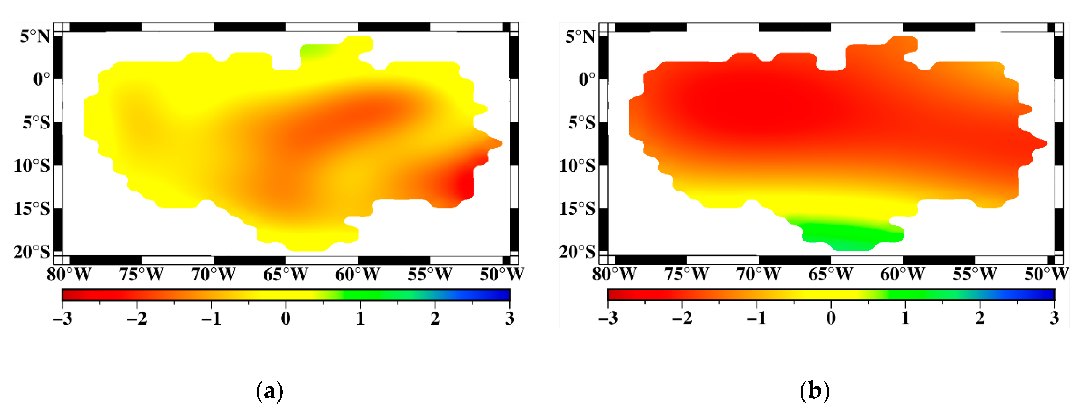
The long-term trend change map of TWSC from the GRACE and Swarm models from December 2013 to May 2020 are shown in Figure 9. The left map is the results from GRACE and the right map is the results from Swarm. There are the similar signals in the southeast and central regions; however, the difference of the signals is more obvious in the most regions. This is because the long-term trend signals in the Amazon basin is weak [37]. If the long-term trend change signals are strong, they can be detected by the Swarm. It shows that the Swarm is suitable for detection in areas with strong signals.
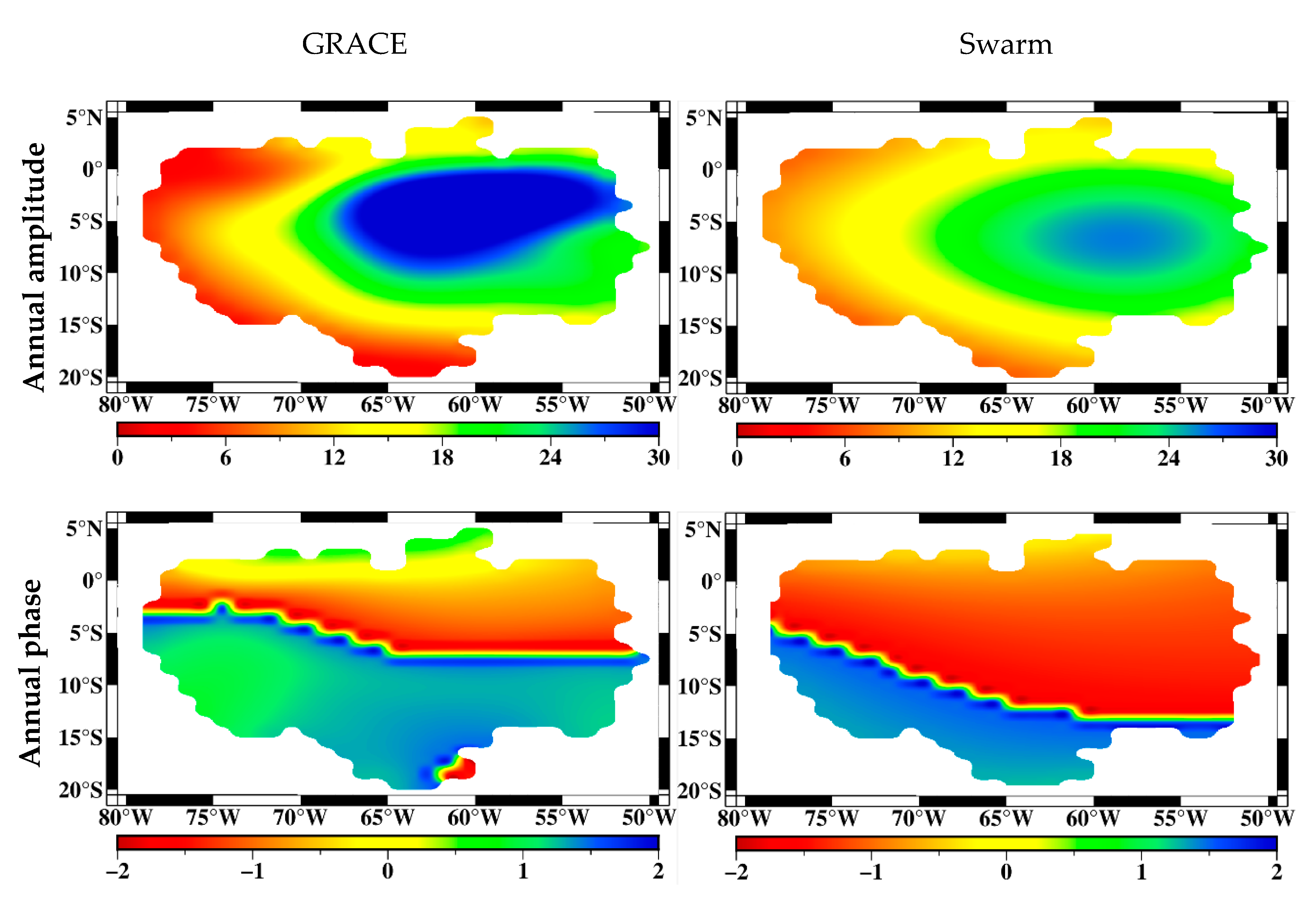
The seasonal changes (annual amplitude and annual phase) of TWSC derived from GRACE and Swarm models covering the period from December 2013 to May 2020 were also compared (Figure 10). The results show that the annual amplitude and annual phase of the two models were similar in terms of the spatial distribution of positive and negative values. According to the annual amplitude maps, the signal strength of GRACE was larger than that of Swarm. The weighted average values of the annual amplitude derived from GRACE and Swarm models are 18.99 and 17.15 cm. It can be seen that there is little difference between the two models. More detail could be seen in the results from GRACE. However, the results of the two models showed some difference in the north and south regions in terms of annual phase.
5. Discussion
This paper compares the GRACE and Swarm TVGF models in detail form two aspects—the SH coefficients of TVGF and the TWSC inversion results—in order to study the potential of using Swarm models data to detect TWSC in the Amazon River basin. Since the successful launch of the Swarm satellites in November 2013, a large number of research institutions have used the hl-SST data of the Swarm satellites to obtain corresponding TVGF models in order to extract geophysical signals [29,31,56,57,58].
However, due to the limitations of this hl-SST data, the precision of the Swarm TVGF model is lower than that of GRACE. We thus need to evaluate how many real signals contained in the Swarm model can be used for TWSC inversion. The degree-error RMS of time-variable signals from the Swarm and GRACE models (Figure 3) show that the model errors of all Swarm models can reach the accuracy level of GRACE model below degree 10. This is because low-degree SH coefficients reflect larger-scale geophysical signals, of which the signal strength is large and easy to detect. The spatial resolution of Swarm models is much lower than that of the GRACE model, so the time-variable field signals that they can see together are mainly concentrated in the low-order parts of the SH coefficients. As the degree increases, the proportion of real signals detected by the Swarm in the total signals is getting increasingly smaller and that of the noise signals is increasingly larger. Therefore, the difference between the degree variances of the time-variable gravity signals derived from these two models becomes bigger. This also shows that the noise levels are growing and dominate the results. The results of degree correlation coefficients between the Swarm and GRACE models (Figure 5) lead to a similar conclusion. Thus, considering the results shown in Figure 3 and Figure 5, the degree of Swarm models used for obtaining the time-variable gravity signals should be truncated to 17 [36,38].
The COST-G-Swarm model was introduced into this study. According to the comparison results of multiple indicators (degree-error RMS, degree variance of time-variable signals, the residual gravity relative to GRACE model and degree correlation), the combination model is better than a single model. It is thus recommended to use the COST-G-Swarm model in future research. COST-G was established at the 2019 General Assembly of the International Union of Geodesy and Geophysics (IUGG), which is a new Product Center of IAG’s International Gravity Field Service (IGFS) for time-variable gravity fields [59]. These models provide consolidated monthly global gravity fields in terms of SH coefficients, such as Swarm and GRACE. These combination models help to further improve the accuracy of the TVGF model and enable us to detect more subtle mass changes in the Earth’s surface or interior.
In the comparison of filtering results between Swarm and GRACE (Figure 6), the stripe errors of the Swarm model were worse than those of the GRACE model [27]. In order to ensure the balance between weakening the stripe errors and retaining the real signals, we suggest the use of 700 km fan filtering to process the Swarm data.
Figure 7 shows the time series of TWSC in the Amazon River basin as calculated by the GRACE and Swarm models. It can be seen that the time series of TWSC has obvious periodic changes (seasonal changes). It was able to clearly reflect several major natural disasters (such as drought events in 2005, 2010 and 2016 and flood events in 2009 and 2012) [51]. Among these, the 2015–2016 drought events occurred during the joint missions of Swarm and GRACE. According to the results, the Swarm and GRACE satellites both detected the occurrence of this event. In this study, the spatial distribution of long-term trend changes and annual changes calculated by the Swarm and GRACE models were compared. The comparison shows a certain similarity in terms of spatial distribution of annual changes (Figure 10), and the values of annual changes are close (Table 2). The TWSC in the Amazon River basin shows a decreasing trend overall (Table 2) [60,61].
6. Conclusions
In this study, we discussed in detail the possibility and effectiveness of the Swarm TVGF model used for quantifying and monitoring TWSC in the Amazon River basin, in order to bridge the data gap between GRACE and GRACE-FO. Firstly, the Swarm TVGF models issued by different institutions were compared and analyzed through various accuracy indicators. The comparison revealed that the ASU-Swarm model has the best accuracy among all single models, but COST-G-Swarm, a combination model, was better than any single model. At the same time, when using the SH coefficient method to calculate the time-variable gravity changes of the Swarm model, it was reasonable to truncate the SH coefficients to degree 17. Combining the above results and filtering efforts, the noise in the Swarm models was greater than that observed in the GRACE model. Subsequently, the comparison of time series, long-term trend changes and annual changes of TWSC in the Amazon River basin proved that the Swarm model has the ability to obtain time-variable gravity signals on the Earth’s surface mass changes in a local region. Compared to previous research, we focused on the spatial distribution of long-term trend changes and seasonal changes of TWSC results from the two models. The results show that the Swarm can fill the data gap between GRACE and GRACE-FO in the detection of long-wave signals in the case of a spatial resolution of 1200 km.
The results of this study can provide a way to fill the data gap between GRACE and GRACE-FO. However, there are still some shortcomings in this study that need to be considered in the future. For example, the application of Swarm in ice sheet quality and gravity changes.
Author Contributions
L.C. and X.W. conceived and designed the research; L.C. and Z.S. performed the experiments and data processing; L.C., B.Z. and Z.L. analyzed the data; L.C. wrote the article; X.W. and Z.Z. revised the article and B.Z. was responsible for funding acquisition. All authors have read and agreed to the published version of the manuscript.
Funding
This research was funded by the National Key R&D Program of China (Grant No. 2018YFC1503503), the National Natural Science Foundation of China (Grant Nos. 41931074, 41974015), the project funded by the Key Laboratory of Geospace Environment and Geodesy, Ministry of Education, Wuhan University (Grant No. 16-01-04, 18-02-04) and The Pre-research Project of Civil Aerospace (Grant No. D010103).
Acknowledgments
We are grateful to CSR for providing the GRACE and GRACE FO monthly gravity field models, AIUB, ASU at Graz University of Technology, IfG at Graz University of Technology and COST-G for providing the Swarm monthly gravity field models, NASA and NOAA for providing the GLDAS model.
Conflicts of Interest
The authors declare no conflict of interest.
References
- Kornfeld, R.P.; Arnold, B.W.; Gross, M.A.; Dahya, N.T.; Klipstein, W.M.; Gath, F.P.; Bettadpur, S. GRACE-FO: The gravity recovery and climate experiment follow-on mission. J. Spacecr. Rockets 2019, 56, 931–951. [Google Scholar] [CrossRef]
- Wahr, J.; Molenaar, M.; Bryan, F. Time variability of the Earth’s gravity field: Hydrological and oceanic effects and their possible detection using GRACE. J. Geophys. Res. 1998, 103, 30205–30229. [Google Scholar] [CrossRef]
- Li, Q.; Luo, Z.C.; Zhong, B.; Wang, H.H. Terretrial water storage change of the 2010 southwest China drought detected by GRACE temporal gravity filed. Chin. J. Geophys. 2013, 56, 1843–1849. (In Chinese) [Google Scholar]
- Chen, J.L.; Wilson, C.R.; Blankenship, D.D.; Tapley, B.D. Antarctic mass rates from GRACE. Geophys. Res. Lett. 2006, 33, L11502. [Google Scholar] [CrossRef] [Green Version]
- Luo, Z.C.; Li, Q.; Zhang, K.; Wang, H.H. Trend of mass changes in the Antarctic ice sheet recovered from the GRACE temporal gravity field. Sci. China Earth Sci. 2012, 55, 76–82. [Google Scholar] [CrossRef]
- Swenson, S.; Chembers, D.; Wahr, J. Estimating geocenter variations from a combination of GRACE and ocean model output. J. Geophys. Res. 2008, 113, B08410. [Google Scholar] [CrossRef] [Green Version]
- Chambers, D.; Wahr, J.; Nerem, R. Preliminary observations of global ocean mass variations with GRACE. Geophys. Res. Lett. 2004, 31, L13310. [Google Scholar] [CrossRef] [Green Version]
- Han, S.C.; Sauber, J.; Riva, R. Contribution of satellite gravimetry to understanding seismic source processes of the 2011 Tohoku-Oki earthquake. Geophys. Res. Lett. 2011, 38, L24312. [Google Scholar] [CrossRef]
- Han, S.C.; Riva, R.; Sauber, J.; Okal, E. Source parameter inversion for recent great earthquakes from a decade-long obervation of global gravity field. J. Geophys. Res. 2013, 118, 1240–1267. [Google Scholar] [CrossRef] [Green Version]
- Zou, Z.B.; Luo, Z.C.; Wu, H.B.; Shen, C.Y.; Li, H. Gravity changes observed by GRACE before the Japan Mw9.0 Earthquake. Acta Geod. Cartogr. Sin. 2012, 41, 171–176. [Google Scholar]
- Tapley, B.D.; Bettadpur, S.; Ries, J.C.; Thompson, P.F.; Watkins, M.M. GRACE measurements of mass variability in the Earth system. Science 2004, 305, 503–505. [Google Scholar] [CrossRef] [PubMed] [Green Version]
- Chen, M.K.; Shum, C.K.; Tapley, B.D. Determination of long-term changes in the Earth’s gravity field from satellite laser ranging observations. J. Geophys. Solid Earth 1997, 102, 22377–22390. [Google Scholar] [CrossRef]
- Cheng, M.; Tapley, B.D. Seasonal variations in low degree zonal harmaonics of the Earth’s gravity field from satellite laser ranging observations. J. Geophys. Res. Solid Earth 1999, 104, 2667–2681. [Google Scholar] [CrossRef]
- Cheng, M.; Tapley, B.D. Variations in the Earth’s oblatenness during the past 28 years. J. Geophys. Res. Solid Earth 2004, 109, B09402. [Google Scholar] [CrossRef]
- Talpe, M.J.; Nerem, R.S.; Forootan, E.; Schmidt, M.; Lemoine, F.G.; Enderlin, E.M.; Landerer, F.W. Ice mass change in Greenland and Antarctica between 1993 and 2013 from satellite gravity measurements. J. Geod. 2017, 91, 1283–1298. [Google Scholar] [CrossRef] [Green Version]
- Haberkorn, C.; Bloßfeld, M.; Bouman, J.; Fuchs, M.; Schmidt, M. Toward a consistent estimation of the earth’s gravity field by combining normal equation matrices from GRACE and SLR. In IAG 150 Year; Springer: Berlin, Germany, 2015; pp. 375–381. [Google Scholar]
- Olsen, N.; Friis-Christensen, E.; Floberhagen, R.; Alken, P.; Beggan, C.D.; Chulliat, A.; Doornbos, E.; da Encarnacan, J.T.; Hamilton, B.; Hulot, C.; et al. The Swarm Satellite Constellation Application and Research Facility (SCARF) and Swarm data products. Earth Planets Space 2013, 65, 1189–1200. [Google Scholar] [CrossRef]
- ESA. Swarm-The Earth’s magnetic field and environment explorers. ESA Rep. SP 2004. [Google Scholar]
- Zangerl, F.; Griesaucr, F.; Sust, M.; Montenbruck, O.; Buckert, B.; Garcia, A. SWARM GPS Precise Orbit Determination Receiver Initial In-Orbit Performance Evaluation. In Proceedings of the 27th International Technical Meeting of the Satellite Division of the Institute of Navigation, Tampa, FL, USA, 8–12 September 2014; pp. 1459–1468. [Google Scholar]
- Van den IJssel, J.; Encarnacao, J.; Doornbos, E.; Visser, P. Precise science orbit for the Swarm satellite constellation. Adv. Space Res. 2015, 56, 1042–1055. [Google Scholar] [CrossRef]
- Prange, L. Global Gravity Field Determination Using the GPS Measurements Made Onboard the Low Earth Orbiting Satellite CHAMP; Schweizerische Geodätische kommission/Swiss Geodetic Commission: Zürich, Switzerland, 2010. [Google Scholar]
- Lin, T.J.; Hwang, C.; Tseng, T.P.; Chao, B.F. Low-degree gravity changes from GPS data of COSMIC and GRACE satellite missions. J. Geodyn. 2012, 53, 34–42. [Google Scholar] [CrossRef]
- Baur, O. Greenland mass variation from time-variable gravity in the absence of GRACE. Geophys. Res. Lett. 2013, 40, 4289–4293. [Google Scholar] [CrossRef]
- Weigelt, M.; van dam, T.; Baur, O.; Tourian, M.J.; Steffen, H.; Sosnica, K.; Jäggl, A.; Zehentner, N.; Mayer-Gürr, T.; Sneeuw, N. How well can the combination of hl-SST and SLR replace GRACE? A discussion from the point of view of applications. In Proceedings of the Grace Science Team Meeting 2014, Potsdam, Germany, 29 September–01 October 2014. [Google Scholar]
- Visser, P.N.A.M.; van der Wal, W.; Schrama, E.J.O.; van den IJssel, J.; Bouman, J. Assessment of observing time-variable gravity from GOCE GPS and accelerometer observations. J. Geod. 2014, 88, 1029–1046. [Google Scholar] [CrossRef]
- Wang, Z.T.; Chao, N.F. Time-variable gravity signal in Greenland revealed by SWARM high-low Satellite-to-Satellite Tracking. Chin. J. Geophys. 2014, 57, 3117–3128. (In Chinese) [Google Scholar]
- Wang, X.X.; Gerlach, C.; Rummel, R. Time-variable gravity field from satellite constellations using the energy integral. Geophys. J. Int. 2012, 190, 1507–1525. [Google Scholar] [CrossRef] [Green Version]
- Bezděk, A.; Sebera, J.; Klokočník, J.; Kostelecky, J. Gravity field models from kinematic orbits of CHAMP, GRACE and GOCE satellites. Adv. Space Res. 2014, 53, 412–429. [Google Scholar] [CrossRef]
- Bezděk, A.; Sebera, J.; Teixeira da Encarnação, J.; Klokocnik, J. Time-variable gravity fields derived from GPS tracking of Swarm. Geophys. J. Int. 2016, 205, 1665–1669. [Google Scholar] [CrossRef] [Green Version]
- Beutle, G.; Jäggi, A.; Mervart, L.; Meyer, U. The celestial mechanics approach: Theoretical foundations. J. Geod. 2010, 84, 605–624. [Google Scholar] [CrossRef] [Green Version]
- Jäggi, A.; Dahle, C.; Arnold, D.; Bock, H.; Meyer, U.; Beutler, G.; van den IJssel, J. Swarm kinematic orbits and gravity fields from 18 months of GPS data. Adv. Space Res. 2016, 57, 218–233. [Google Scholar] [CrossRef]
- Ilk, K.H.; Mayer-Gürr, T.; Feuchtinger, M. Gravity Field Recovery by Analysis of Short Arcs of CHAMP//Earth Observation with CHAMP; Springer: Berlin/Heidelberg, Germany, 2005; pp. 127–132. [Google Scholar]
- Weigelt, M.; van Dam, T.; Jäggi, A.; Prange, L.; Tourian, M.J.; Keller, W.; Sneeuw, N. Time-variable gravity signal in Greenland revealed by high-low satellite-to-satellite tracking. J. Geophys. Res. Solid Earth 2013, 118, 3848–3859. [Google Scholar] [CrossRef] [Green Version]
- Lück, C.; Kusche, J.; Rietbroek, R.; Löcher, A. Time-variable gravity fields and ocean mass change from 37 months of kinematic Swarm orbits. Solid Earth 2018, 9, 323–339. [Google Scholar] [CrossRef] [Green Version]
- Wang, X.L. Study on Extraction Method and Application of Time-Variable Gravity Signal Detected by Satellite. Ph.D. Thesis, Wuhan University, Wuhan, China, 2019. [Google Scholar]
- Da Encarnação, T.J.; Arnold, D.; Bezděk, A.; Dahle, C.; Doornbos, E.; van den IJssel, J.; Jäggi, A.; Mayer-Gürr, T.; Sebera, J.; Visser, P.; et al. Gravity field models derived from Swarm GPS data. Earth Planets Space 2016, 68, 127. [Google Scholar] [CrossRef] [Green Version]
- Da Encarnação, T.J.; Visser, P.; Arnold, D.; Bezděk, A.; Doornbos, E.; Ellmer, M.; Guo, J.Y.; van den IJssel, J.; Iorfida, E.; Jäggi, A.; et al. Description of the multi-approach gravity field models from Swarm GPS data. Earth Syst. Sci. Data 2020, 12, 1385–1417. [Google Scholar] [CrossRef]
- Fan, Y.; Miguez-Macho, G. Potential groundwater contribution to Amazon evapotranspiration. Hydrol. Earth Syst. Sci. 2009, 14, 2039–2056. [Google Scholar] [CrossRef] [Green Version]
- Latrubesse, E.M.; Arima, E.Y.; Dunne, T.; Park, E.; Baker, V.R.; d’Hort, F.M.; Wight, C.; Wittmann, F.; Zuanon, J.; Baker, P.A.; et al. Damming the rivers of the Amazon basin. Nature 2017, 546, 363–369. [Google Scholar] [CrossRef]
- Malhi, Y.; Roberts, J.T.; Betts, R.A.; Killeen, T.J.; Li, W.; Nobre, C.A. Climate change, deforestaion, and the fate of the Amazon. Science 2008, 319, 169–172. [Google Scholar] [CrossRef] [Green Version]
- Nobre, C.A.; Sellers, P.J.; Shukla, J. Amazonian deforestation and regional climate change. J. Clim. 1991, 4, 957–988. [Google Scholar] [CrossRef] [Green Version]
- Chaudhari, S.; Pokhrel, Y.; Moran, E.; Miguez-Macho, G. Muti-decadal hydrologic change and variability in the Amazon River basin: Understanding terrestrial water storage variations and drought characteristics. Hydrol. Earth Syst. Sci. 2019, 23, 2841–2862. [Google Scholar] [CrossRef] [Green Version]
- Swenson, S.; Wahr, J. Post-processing removal of correlated errors in GRACE data. Geophys. Res. Lett. 2006, 33, L08402. [Google Scholar] [CrossRef]
- Jean, Y.; Meyer, U.; Jäggi, A. Combination of GRACE monthly gravity field solutions from different processing strategies. J. Geod. 2018, 92, 1313–1328. [Google Scholar] [CrossRef] [Green Version]
- Rodell, M.; Houser, P.; Jambor, U.E.A.; Gottschalck, J.; Mitchell, K.; Meng, C.; Arsenault, K.; Cosgrove, B.; Radakovich, J.; Bosilovich, M. The global land data assimilation system. Bull. Am. Meteorol. Soc. 2004, 85, 381–394. [Google Scholar] [CrossRef] [Green Version]
- Chen, J.L.; Wilson, C.R.; Famiglietti, J.S.; Rodell, M. Spatial sensitivity of the Gravity Recovery and Climate Experiment(GRACE) time-variable gravity observations. J. Geophys. Res. Solid Earth 2006, 111, 115–139. [Google Scholar] [CrossRef] [Green Version]
- Zhou, X.H.; Xu, H.Z.; Wu, B.; Peng, B.B.; Lu, Y. Earth’s gravity field derived from GRACE satellite tracking data. Chin. J. Geophys. 2006, 49, 718–723. [Google Scholar] [CrossRef]
- Zhang, Z.; Chao, B.; Chen, J.L.; Wilson, C. Terrestrial water storage anomalies of Yangtze River basin droughts observed by GRACE and Connections with ENSO. Glob. Planet Chang. 2015, 126, 35–45. [Google Scholar] [CrossRef]
- Wang, X.L.; Luo, Z.C.; Zhong, B.; Wu, Y.H.; Huang, Z.K.; Zhou, H.; Li, Q. Separation and recovery of geophysical signals based on the Kalman filter with GRACE gravity data. Remote Sens. 2019, 11, 393. [Google Scholar] [CrossRef] [Green Version]
- Zhang, Z.Z.; Chao, B.F.; Yang, L.; Hsu, H.T. An effective filtering for GRACE time-variable gravity: Fan filter. Geophys. Res. Lett. 2009, 36, L17311. [Google Scholar] [CrossRef]
- Li, F.P.; Wang, Z.T.; Chao, N.F.; Feng, J.D.; Zhang, B.B.; Tian, K.J.; Han, Y.K. 2015–2016 drought event in the Amazon River Basin as measured by Swarm constellation. Geomat. Inf. Sci Wuhan Univ. 2020, 45, 595–603. [Google Scholar]
- Chen, J.L.; Wilson, C.R.; Tapley, B.D.; Yang, Z.L.; Niu, G.Y. 2005 drought event in the Amazon River basin as measured by GRACE and estimated by climate models. J. Geophys. Res. 2009, 114, B05404. [Google Scholar] [CrossRef]
- Panisset, J.S.; Libonati, R.; Gouveia, C.M.P.; Silva, F.M.; Franca, D.A.; Franca, J.R.A.; Peres, L.F. Contrasting patterns of the extreme drought episodes of 2005, 2010 and 2015 in the Amazon Basin. Int. J. Clinatol. 2018, 38, 1096–1104. [Google Scholar] [CrossRef]
- Chen, J.L.; Wilson, C.R.; Tapley, B.D. The 2009 exceptional Amazon flood and interannual terretrial water storage observed by GRACE. Water Storage Res. 2010, 46, 439–445. [Google Scholar]
- Nie, N.; Zhang, W.; Guo, H. 2010–2012 drougt and flood events in Amazon River Basin inferred by GRACE satellite observations. J. Appl. Remote Sens. 2015, 9, 096023. [Google Scholar] [CrossRef]
- Zehentner, N.; Mayer-Gürr, T. Precise orbit determination based on raw GPS measurement. J. Geod. 2016, 90, 275–286. [Google Scholar] [CrossRef] [Green Version]
- Guo, J.Y.; Shang, K.; Jekeli, C.; Shum, C.K. On the energy integral formulation of gravitational potential differences from satellite-to-satellite tracking. Celest. Mech. Dyn. Astr. 2015, 121, 415–429. [Google Scholar] [CrossRef]
- Zhang, B.B. Precise Orbit Determination and the Earth Gravity Field Recovery by Acceleration Approach for Swarm. Ph.D. Thesis, Wuhan University, Wuhan, China, 2017. [Google Scholar]
- Jäggi, A.; Meyer, U.; Lasser, M.; Jenny, B.; Lopez, T.; Flechtner, F.; Dahle, C.; Förste, C.; Mayer-Gürr, T.; Kvas, A.; et al. International Combination Service for Time-variable Gravity Fields (COST-G)—Start of operational phase and future perspectives. In IAG Symposia; Springer: Berlin/Heidelberg, Germany, 2020. [Google Scholar] [CrossRef]
- Christopher, E.N.; Vagner, G.F. Assessing land water storage dynamics over South America. J. Hydrol. 2020, 580, 124339. [Google Scholar]
- Forootan, E.; Schumacher, M.; Mehrnegar, N.; Bezděk, A.; Talpe, M.J.; Farzeneh, S.; Zhang, C.Y.; Zhang, Y.; Shum, C.K. An iterative ICA-based reconsyruction method to produce consisitent time-variable total water storage fields using GRACE and Swarm Satellite Data. Remote Sens. 2020, 12, 1639. [Google Scholar] [CrossRef]
Figure 1.
Amazon River basin (the red curve is the basin boundary and the bold line is the main stream).
Figure 1.
Amazon River basin (the red curve is the basin boundary and the bold line is the main stream).

Figure 2.
Internal coincidence accuracy of Gravity Recovery and Climate Experiment (GRACE) and Swarm models.
Figure 2.
Internal coincidence accuracy of Gravity Recovery and Climate Experiment (GRACE) and Swarm models.

Figure 3.
External coincidence accuracy of GRACE and Swarm models.

Figure 4.
Degree-error root mean square (RMS) of the residual values of spherical harmonic (SH) coefficients of Swarm monthly gravity field relative to the GRACE model.
Figure 4.
Degree-error root mean square (RMS) of the residual values of spherical harmonic (SH) coefficients of Swarm monthly gravity field relative to the GRACE model.

Figure 5.
Degree correlation between Swarm and the GRACE models (left column is C coefficient results and right column is S coefficient results).
Figure 5.
Degree correlation between Swarm and the GRACE models (left column is C coefficient results and right column is S coefficient results).

Figure 6.
C20 time series.

Figure 7.
Monthly surface mass variation on March 2016 with unfiltered (top row), 300 km fan filter (second row), 500 km fan filter (third row) and 700 km fan filter (bottom row) from GRACE (left column) and Swarm (right column).
Figure 7.
Monthly surface mass variation on March 2016 with unfiltered (top row), 300 km fan filter (second row), 500 km fan filter (third row) and 700 km fan filter (bottom row) from GRACE (left column) and Swarm (right column).

Figure 8.
The terrestrial water storage change (TWSC) time series in the Amazon River basin calculated using GRACE (blue curve) and Swarm (green curve).
Figure 8.
The terrestrial water storage change (TWSC) time series in the Amazon River basin calculated using GRACE (blue curve) and Swarm (green curve).

Figure 9.
Long-term trends of TWSC in the Amazon River basin calculated by GRACE and Swarm. (a) GRACE results; (b) Swarm results.
Figure 9.
Long-term trends of TWSC in the Amazon River basin calculated by GRACE and Swarm. (a) GRACE results; (b) Swarm results.

Figure 10.
TWSC seasonal changes in the Amazon River basin calculated by GRACE and Swarm.


Table 1.
Comparisons of Swarm time-variable gravity (TVG) data solutions from different institutes.
| Institute | AIUB | ASU | IfG | COST-G |
|---|---|---|---|---|
| Orbit | AIUB | ITSG | IfG | Combination |
| Approach | Celestial mechanics | Acceleration | Short-arc | Combination |
| Highest order | 70 | 40 | 40 | 40 |
| Time span | 2014.01–2016.12 | 2013.12–2020.05 | 2013.11–2016.12 | 2013.12–2020.05 |
| Download address | ftp://ftp.aiub.unibe.ch/GRAVITY/SWARM/ | http://www.asu.cas.cz/~bezdek/vyzkum/geopotencial/index.php | http://ftp.tugraz.at/outgoing/ITSG/tvgogo/gravityFieldModels | http://icgem.gfz-potsdam.de/series/02_COST-G/Swarm |
Table 2.
Long-term trends and seasonal changes from Swarm and GRACE TVG field. AA and AP present the annual amplitude and annual phase, respectively.
Table 2.
Long-term trends and seasonal changes from Swarm and GRACE TVG field. AA and AP present the annual amplitude and annual phase, respectively.
| Model | Time Span | Long-Term Trend (cm/a) | AA (cm) | AP (rad) |
|---|---|---|---|---|
| GRACE | 2013.12–2020.05 | −0.72 | 15.65 | −1.36 |
| Swarm | −1.50 | 16.39 | −1.33 |
Publisher’s Note: MDPI stays neutral with regard to jurisdictional claims in published maps and institutional affiliations. |
© 2020 by the authors. Licensee MDPI, Basel, Switzerland. This article is an open access article distributed under the terms and conditions of the Creative Commons Attribution (CC BY) license (http://creativecommons.org/licenses/by/4.0/).
Share and Cite
MDPI and ACS Style
Cui, L.; Song, Z.; Luo, Z.; Zhong, B.; Wang, X.; Zou, Z. Comparison of Terrestrial Water Storage Changes Derived from GRACE/GRACE-FO and Swarm: A Case Study in the Amazon River Basin. Water 2020, 12, 3128. https://doi.org/10.3390/w12113128
AMA Style
Cui L, Song Z, Luo Z, Zhong B, Wang X, Zou Z. Comparison of Terrestrial Water Storage Changes Derived from GRACE/GRACE-FO and Swarm: A Case Study in the Amazon River Basin. Water. 2020; 12(11):3128. https://doi.org/10.3390/w12113128
Chicago/Turabian StyleCui, Lilu, Zhe Song, Zhicai Luo, Bo Zhong, Xiaolong Wang, and Zhengbo Zou. 2020. "Comparison of Terrestrial Water Storage Changes Derived from GRACE/GRACE-FO and Swarm: A Case Study in the Amazon River Basin" Water 12, no. 11: 3128. https://doi.org/10.3390/w12113128
Note that from the first issue of 2016, this journal uses article numbers instead of page numbers. See further details here.