Optimization Assessment of Projection Methods of Climate Change for Discrepancies between North and South China

Abstract

Downscaling methods have been widely used due to the coarse and biased outputs of general circulation models (GCMs), which cannot be applied directly in regional climate change projection. Hence, appropriate selection of GCMs and downscaling methods is important for assessing the impacts of climate change. To explicitly explore the influences of multi-GCMs and different downscaling methods on climate change projection in various climate zones, the Heihe River Basin (HRB) and the Zhanghe River Basin (ZRB) were selected in this study to represent the north arid region and the south humid region in China, respectively. We first evaluated the performance of multi-GCMs derived from Coupled Model Inter-comparison Project Phase 5 (CMIP5) in the two regions based on in-situ measurements and the 40 year European Centre for Medium-Range Weather Forecasts (ECMWF) Re-Analysis (ERA-40) data. Subsequently, to construct appropriate climate change projection techniques, comparative analysis using two statistical downscaling methods was performed with consideration of the significant north–south meteorological discrepancies. Consequently, specific projections of future climate change for 2021–2050 under three representative concentration pathway (RCP) scenarios (RCP2.6, RCP4.5, and RCP8.5) were completed for the HRB and ZRB, including daily precipitation, maximum air temperature, and minimum air temperature. The results demonstrated that the score-based method with multiple criteria for performance evaluation of multiple GCMs more accurately captured the spatio-temporal characteristics of the regional climate. The two statistical downscaling methods showed respective advantages in arid and humid regions. The statistical downscaling model (SDSM) showed more accurate prediction capacities for air temperature in the arid-climate HRB, whereas model output statistics (MOS) better captured the probability distribution of precipitation in the ZRB, which is characterized by a humid climate. According to the results obtained in this study, the selection of appropriate GCMs and downscaling methods for specific climate zones with different meteorological features significantly impact regional climate change projection. The statistical downscaling models developed and recommended for the north and south of China in this study provide scientific reference for sustainable water resource management subject to climate change.

1. Introduction

According to the fifth assessment report of the Intergovernmental Panel on Climate Change (IPCC), the global mean temperature will continue rising until the end of the 21st century, associated with a significant increase in the frequency and intensity of extreme climate events, which will cause severe socio-economic upheaval and environmental degradation [1,2,3,4]. As one of the countries suffering from the significant impacts of climate change, China has an unequivocally urgent need for accurate projections of climate change, which are seriously limited by regional heterogeneities in climate and anthropogenic activities. Hence, development of projection methods that suitably capture spatio-temporal characteristics of regional climate change has become a key scientific issue to address the impact of global climate change at the regional scale. General circulation models (GCMs) are major tools used to provide large-scale information for the impact assessment of global climate change; however, their coarse spatial resolution and biased outputs hinder their direct application to climate change prediction at the regional scale [5,6,7]. Consequently, dynamic and statistical downscaling methods have been developed to mitigate the mismatch in spatial scales and biases between GCM outputs and in-situ measurements. Dynamic downscaling methods, i.e., regional climate models (RCMs), have been developed based on dynamic formulations using initial and time-dependent lateral boundary conditions of GCMs to generate finer-resolution climate data, which provide more detailed regional information and have been widely used worldwide [8,9,10]. However, complexity exists in the computation and mismatch of scales, especially for small-scale watersheds [11,12,13]. Conversely, statistical downscaling methods primarily establish statistical relationships between large-scale predictors and local-scale predictands without physical representation or parameterization, being simple to compute and relatively easy to implement [7,14,15,16,17,18]. These methods have been widely and successfully used in regional climate change projections. The distinct internal mechanisms of different statistical downscaling methods are one of the main sources of uncertainty in climate change projection. For example, Chiew et al. [19] selected three downscaling models with increasing complexity to investigate the difference between the modeled future runoff using the different downscaled rainfall. The results revealed that the differences in the results can be significant due to different GCMs and different methods. Cheng et al. [20] developed statistical extreme weather event simulation and downscaling models for southern-central Canada; they employed different regression methods for different meteorological variables considering the adaptability of the methods. Sunyer et al. [21] used eight statistical methods to downscale precipitation outputs from 15 RCMs in Europe to highlight the need to consider an ensemble of both methods and climate models. In addition, Yang et al. [7] investigated the performance of four statistical downscaling methods to improve the accuracy of GCMs in terms of spatial variability. Other researchers also conducted comparative studies of methods in China. For example, Liu et al. [22] used the nonhomogeneous hidden Markov model (NHMM) and statistical downscaling model (SDSM) to downscale precipitation over an arid region in China and found that their abilities to simulate wet-day precipitation amounts differed—NHMM performed better. In addition, Hu et al. [23] compared three statistical methods to downscale summer daily precipitation over the Yellow River source region to illustrate the strengths and weaknesses of different methods in terms of several statistics. Similar studies were performed in the Yangtze River Basin and the North China Plain [24,25]. Most of the studies mainly aimed at the same type of region to compare different downscaling methods to investigate their advantages, but few studies have focused on the selection of downscaling methods due to the climate characteristics of different regions, which is important for reducing the uncertainty in climate change projection.

Many studies have consistently pointed out that the uncertainty from GCMs is also critical for climate change projection, which could be efficiently reduced by multi-model averaging. Rana and Moradkhani [26] chose 10 GCMs from Coupled Model Inter-comparison Project Phase 5 (CMIP5) and used two statistical downscaling methods (bias correction and spatial downscaling, multivariate adaptive constructed analogs) to examine the spatial and temporal changes in precipitation and temperature over the Columbia River Basin. The results could be used to help planners to better understand the range of possible future climate change effects by considering multi-model projection, rather than a single GCM. San-Martin et al. [27] compared the spread uncertainty of GCMs and downscaling methods, indicating that of the latter can be greater. Zelazowski et al. [28] presented a pattern-scaling set to scan uncertainty in climate models, but the ability to capture the course of uncertainty remains a limitation. More recently, Kusangaya et al. [29] found that the ability of downscaled GCMs to capture the spatial variability of extreme hydrological events contains considerable uncertainty. Tegegne et al. [30] proposed a new approach to combine multiple GCMs to increase the reliability of climate predictions. However, multi-model ensemble projection, without considering specific performance assessment at the regional scale, cannot concisely depict the regional climate characteristics; due to the significant spatio-temporal heterogeneities of regional climate change, the relative uncertainty of the contribution of each impact assessment stage can vary depending on the projection variable and the method used to examine the uncertainty [31,32].

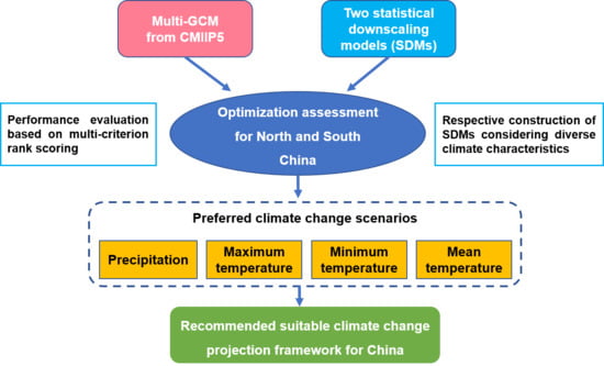
Wang et al. [33] explored the projections of future climate change in the Heihe River Basin by constructing a statistical downscaling model (SDSM). They built a good study framework, but it was aimed at a specific arid area and did not provide suggestions for the discrepancy between South and North China. In this study, to explicitly explore the influences of multi-GCMs and different downscaling methods on climate change projection in various climate zones, we selected the Heihe River Basin (HRB), located in northwestern China, and the Zhanghe River Basin (ZRB), located in the lower reaches of the Yangtze River Basin, to represent the north–south discrepancy in the climate in China. Two statistical downscaling methods, an SDSM and model output statistics (MOS), were constructed for both basins to comparatively analyze the uncertainty in the climate change projections of the downscaling methods. The objectives of this study were (1) to determine suitable GCMs for the HRB and ZRB separately, based on the performance evaluation of multi-GCMs derived from CMIP5 using the score-based method [34,35]; (2) to construct the SDSM and MOS using the 40 year ECMWF Re-Analysis (ERA-40) data and observed meteorological data to investigate the adaptability of the two downscaling methods to different climate zones; and (3) to generate future climate change scenarios by applying the identified preferred downscaling method for the HRB and ZRB under three representative concentration pathway (RCP) scenarios (RCP2.6, RCP4.5, and RCP8.5), determining the variation ranges of different climate variables including precipitation, maximum air temperature, and minimum air temperature. The results obtained provide certain guidance for climate change projection, with an emphasis on the substantial importance of regional differences, and could provide a scientific reference for sustainable water resource management under climate change.

2. Materials and Methods

2.1. Study Area

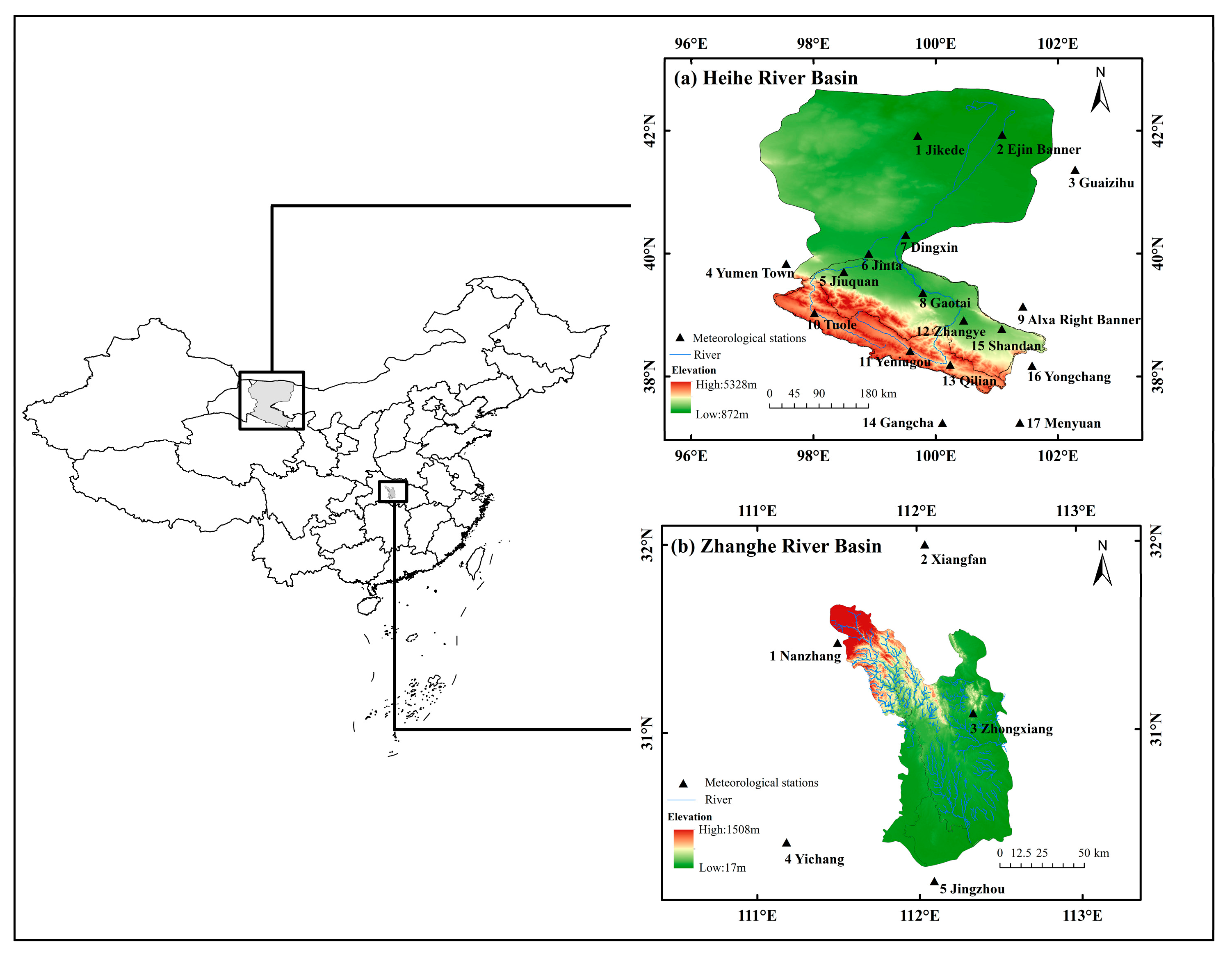
This study was conducted in two basins (the HRB and ZRB) with different hydro-climatic regimes (Figure 1), representing the south–north spatial heterogeneity in China.

2.1.1. Heihe River Basin

The HRB, the second largest inland river basin, is located in the central Hexi Corridor of northwestern China, with coordinates of approximately 98°–101° E and 38°–42° N. Due to the complicated geomorphology and disparity in altitude, the climate characteristics of this area show significant regional differences. The HRB is divided into three parts by the Yingluo Gorge and the Zhengyi Gorge from south to north. Above the Yingluo Gorge are the upper reaches, where the water sources mainly originate; the elevation here ranges from 1680 to 5280 m. The middle reaches are between the two gorges, with relatively flat terrain, containing 90% of the population and agricultural land of the whole basin. The annual mean air temperature and precipitation are 6–8 °C and 120–200 mm, respectively. The lower reaches are below the Zhengyi Gorge, having sparse natural vegetation and an annual mean precipitation of less than 50 mm; this area is one of the main sources of sandstorms in North China [36,37].

2.1.2. Zhanghe River Basin

The ZRB is located in southern-central China, bounded by coordinates spanning 111° to 113° E and 30° to 32° N. It is characterized by a warm and humid subtropical climate. As part of the rainstorm area in the middle reaches of the Yangtze River, the mean annual precipitation of this area is 1000 mm, with extremely uneven annual rainfall distribution, which leads to frequent drought and flood disasters. The Zhanghe reservoir is the boundary of the upper and lower reaches. The lower reaches are dominated by hills, and the total cultivated area is 16.4 × 10⁴ ha, playing an essential role as one of the rice production bases in Hubei Province.

2.2. Data

2.2.1. Observed Data

In this study, in-situ observations from 17 gauged stations in the HRB and five gauged stations in the ZRB, including monthly and daily precipitation and mean, maximum, and minimum air temperature, were obtained from the China Meteorological Data Service Center (http://data.cma.cn/en). The monthly data were used for the performance evaluation of multi-GCMs for the two basins, and the daily data were divided into two periods for statistical downscaling model calibration and validation.

2.2.2. GCM Data

Monthly and daily data of 23 GCMs were obtained from CMIP5 (https://esgf-node.llnl.gov/search/cmip5/) (

Table A2. Information of 23 GCMs from CMIP5.

ID	Model Name	Source	Horizontal Resolution (lat × lon)
1	BCC-CSM 1.1	Beijing Climate Center, China Meteorological Administration, China	2.7906° × 2.8125°
2	BCC-CSM1.1-M	Beijing Climate Center, China Meteorological Administration, China	1.1215° × 1.125°
3	CanESM2	Canadian Centre for Climate Modelling and Analysis, Canada	2.7906° × 2.8125°
4	CCSM4	National Center for Atmospheric Research (NCAR), USA	0.9424° × 1.25°
5	CESM1-CAM5	National Center for Atmospheric Research (NCAR) Boulder, CO, USA	0.9424° × 1.25°
6	CNRM-CM5	Centre National de Recherches Meteorologiques, Meteo-France, France	1.4007° × 1.4063°
7	CSIRO-Mk3.6.0	Australian Commonwealth Scientific and Industrial Research Organization, Australia	1.8653° × 1.875°
8	FGOALS-g2	Institute of Atmospheric Physics, Chinese Academy of Sciences, China	2.7906° × 2.8125°
9	FIO-ESM	The First Institute of Oceanography, SOA, China	2.7906° × 2.8125°
10	GFDL-CM3	Geophysical Fluid Dynamics Laboratory, USA	2° × 2.5°
11	GFDL-ESM2G	Geophysical Fluid Dynamics Laboratory, USA	2° × 2.5°
12	GISS-E2-H	NASA Goddard Institute for Space Studies, USA	2° × 2.5°
13	GISS-E2-R	NASA Goddard Institute for Space Studies, USA	2° × 2.5°
14	HadGEM2-ES	Met Office Hadley Centre, UK	1.25° × 1.875°
15	IPSL-CM5A-LR	Institut Pierre-Simon Laplace, France	1.8947° × 3.75°
16	IPSL-CM5A-MR	Institut Pierre-Simon Laplace, France	1.2676° × 2.5°
17	MIROC5	Atmosphere and Ocean Research Institute (The University of Tokyo),National Institute for Environmental Studies, and Japan Agency for Marine-Earth Science and Technology, Japan	1.4005° × 1.4063°
18	MIROC-ESM	Atmosphere and Ocean Research Institute (The University of Tokyo), National Institute for Environmental Studies, and Japan Agency for Marine-Earth Science and Technology, Japan	2.7906° × 2.8125°
19	MIROC-ESM-CHEM	Atmosphere and Ocean Research Institute (The University of Tokyo), National Institute for Environmental Studies, and Japan Agency for Marine-Earth Science and Technology, Japan	2.7906° × 2.8125°
20	MPI-ESM-LR	Max Planck Institute for Meteorology, Germany	1.8653° × 1.875°
21	MPI-ESM-MR	Max Planck Institute for Meteorology, Germany	1.8653° × 1.875°
22	MRI-CGCM3	Meteorological Research Institute, Japan	1.1215° × 1.125°
23	NorESM1-M	Norwegian Climate Centre, Norway	1.8947° × 2.5°

). The monthly data from the historical experiments were used for performance evaluation of the GCMs, whereas the daily data from the historical and RCP experiments were used to generate future climate change scenarios under three RCP scenarios (RCP2.6, RCP4.6, and RCP8.5) using the statistical downscaling methods. For each GCM, we selected variant label r1i1p1f1. To unify the different spatial resolution of the GCMs, consider the different sizes of the two basins, and ensure each grid captured at least one gauged station, GCM data were resampled to 2° × 2° in the HRB and 1.5° × 1.5° in the ZRB.

2.2.3. ERA-40 Reanalysis Data

The ERA-40 reanalysis data were obtained from the European Centre for Medium-Range Weather Forecasts (ECMWF) [38]. Research continues to demonstrate that ERA-40 reanalysis data are more applicable than other data for simulating the spatio-temporal evolution patterns of precipitation and air temperature in most areas in China. Therefore, daily ERA-40 reanalysis data, including precipitation and air temperature for 1961–2000 from the ECMWF (http://apps.ecmwf.int/datasets/data/era40-daily/levtype=sfc/), were extracted to construct the SDSM model. The spatial resolution of ERA-40 is consistent with that of the GCMs used in the HRB and ZRB.

Notably, due to the inconsistent lengths of the data (observed data: 1961–2005/2006, GCM data: 1961–2005 and ERA-40 reanalysis data: 1961–2000), 1961–1990 and 1991–2000 were set as the calibration and validation periods for the SDSM model, respectively. Due to the MOS model directly establishing the relationship between GCM output and observed climate variables to downscale and correct the biases, 1961–1990 was set as the calibration period, and 1991–2005 and 1991–2006 were set as the validation periods for the preferred GCMs in the HRB and ZRB, respectively. The different length of validation periods is considered as to use the available data as much as possible [39,40].

2.3. Methods

2.3.1. Performance Evaluation of Multi-GCMs

Score-Based Method

Previous studies have found that the simulation performance of each GCM differs significantly, especially for different climate regions [41,42,43]. To identify the preferred GCM for a certain region, a score-based method was applied to the multi-model adaptive assessment in this study. Through this method, in-situ observations of precipitation and mean, maximum, and minimum air temperature were compared with the GCM simulations on a monthly scale based on 11 evaluation metrics (

Table 1. Evaluation metrics used for general circulation model (GCM) performance assessment.

Evaluation Metric	Method
Mean	Relative Error (%)
Coefficient of variation	Relative Error (%)
Temporal variation	Normalized root mean square error (NRMSE) [44]
Monthly distribution	Pearson correlation coefficient [45,46]
Spatial distribution	Pearson correlation coefficient
Trend and its magnitude	Mann–Kendall Z test [47]
	Mann–Kendall β test [48]
Space–time variability	The first eigenvector of empirical orthogonal functions (EOF1) [49,50]
	The second eigenvector of empirical orthogonal functions (EOF2)
Probability density functions (PDFs)	Brier score (BS) [51]
	Skill score (Sscore)

), characterizing climate long-term means and standard deviations, seasonal variation, spatiotemporal distribution, and probability density functions. The multi-criteria rank score (RS) was calculated as follows:

$$R{S}_i=\frac{1}{N}{\displaystyle \sum }_{n=1}^N(\frac{X_{\max }-X_i}{X_{\max }-X_{\min }}\times 10)$$

(1)

where N is the number of evaluation metrics (N = 11), X_i is the relative error between the ith GCM output and the observed climate variable, and X_max and X_min are the respective maximum and minimum values of the relative error. All evaluation metrics have a weight of 1.0 in this study. For each GCM, we calculated an RS for each climate variable. The higher the RS, the better the performance of the GCM.

2.3.2. Statistical Downscaling Methods

SDSM

The statistical downscaling model (SDSM), developed by Wilby et al. [52], is based on the coupling principle of multiple linear regression and the stochastic weather generator [53] and is commonly used in the downscaling of regional climate change and projection of future climate change scenarios [54,55,56]. Its core concept is to establish the empirical relationships between local-scale predictands (observed data) and regional-scale predictors (ERA40 reanalysis data).

The downscaling of daily precipitation and maximum, minimum, and mean air temperature by the SDSM involves five steps: (1) screening of downscaling predictor variables [57,58]. By combining the correlation matrix, partial correlation, and scatter plots, suitable predictors are screened through a multiple linear regression model. The structure of the model has two forms: unconditional and conditional. Precipitation is usually modeled as a conditional process, whereas air temperature is modeled as an unconditional process. (2) The model is calibrated [59] by adjusting the coefficient of variance inflation (VIF, where 0 < VIF < 10 indicates no correlation, 10 < VIF < 100 indicates a moderate correlation, and VIF ≥ 100 indicates a high correlation; the default value is 12) and by bias correction (BC, ranges from 0 to 2. The default value is 1.0, which indicates no bias correction). The outputs of SDSM are calibrated with daily observed data. (3) The weather generator [60,61] operation generates ensembles of synthetic daily weather series given observed (or ERA40 reanalysis) atmospheric predictor variables. The procedure enables the verification of calibrated models (using independent data) and the synthesis of artificial time series for present climate conditions. (4) The model is validated [18,61,62]. (5) Climate scenarios are generated for statistical analyses.

Table A1. Selected predictors according to different variables of the meteorological stations.

Area	Stations	Tmax	Tmin	Tmean	Precipitation
HRB	1 Jikede	mslp, p5ta, p7ta, p8ta, ta2m	mslp, p5ta, p7ta, p8ta, ta2m, p7hu, p8hu	mslp, p5ta, p7ta, p8ta, ta2m	lspr, mslp, p7ta, p8ta, ta2m, p7hu, p8hu
	2 Ejin Banner	mslp, p7ta, p8ta, ta2m	mslp, p5ta, p7ta, p8ta, ta2m, p7hu, p8hu	mslp, p5ta, p7ta, p8ta, ta2m	lspr, p7ta, p8ta, ta2m, p5hu, p7hu, p8hu
	3 Guaizihu	mslp, p7ta, p8ta, ta2m	mslp, p5ta, p7ta, p8ta, ta2m	mslp, p7ta, p8ta, ta2m	lspr, p7ta, p8ta, ta2m, p5hu, p7hu, p8hu
	4 Yumen Town	mslp, p7ta, p8ta, ta2m	mslp, p5ta, p7ta, p8ta, ta2m, p7hu	mslp, p7ta, p8ta, ta2m	lspr, mslp, p7ta, p8ta, ta2m, p7hu, p8hu
	5 Jiuquan	mslp, p7ta, p8ta, ta2m	mslp, p5ta, p7ta, p8ta, ta2m, p7hu	mslp, p7ta, p8ta, ta2m	lspr, mslp, p7ta, p8ta, ta2m, p7hu, p8hu
	6 Jinta	mslp, p7ta, p8ta, ta2m	mslp, p5ta, p7ta, p8ta, ta2m, p7hu, p8hu	mslp, p7ta, p8ta, ta2m	lspr, mslp, p7ta, p8ta, ta2m, p7hu, p8hu
	7 Dingxin	mslp, p7ta, p8ta, ta2m	mslp, p5ta, p7ta, p8ta, ta2m, p7hu, p8hu	mslp, p7ta, p8ta, ta2m	lspr, mslp, p7ta, p8ta, ta2m, p7hu, p8hu
	8 Gaotai	mslp, p7ta, p8ta, ta2m	p5ta, p8ta, ta2m, p7hu, p8hu	mslp, p7ta, p8ta, ta2m	lspr, mslp, p7ta, p8ta, ta2m, p7hu, p8hu
	9 Alxa Right Banner	mslp, p7ta, p8ta, ta2m	mslp, p5ta, p7ta, p8ta, ta2m	mslp, p7ta, p8ta, ta2m	lspr, mslp, p7ta, p8ta, ta2m, p7hu, p8hu
	10 Tuole	mslp, p5ta, p7ta, p8ta, ta2m	p5ta, ta2m, p8hu	p5ta, p7ta, p8ta, ta2m	lspr, mslp, p7ta, p8ta, ta2m, p8hu
	11 Yeniugou	mslp, p5ta, p7ta, p8ta, ta2m	p5ta, ta2m, p5hu, p7hu, p8hu	p5ta, p7ta, p8ta, ta2m	lspr, mslp, p7ta, p8ta, ta2m, p7hu, p8hu
	12 Zhangye	mslp, p7ta, p8ta, ta2m	p5ta, ta2m, p5hu, p7hu, p8hu	mslp, p5ta, p7tap8ta, ta2m	lspr, mslp, p7ta, p8ta, ta2m, p7hu, p8hu
	13 Qilian	mslp, p5ta, p7ta, p8ta, ta2m	ta2m, p5hu, p7hu, p8hu	mslp, p5ta, p7tap8ta, ta2m	lspr, mslp, p7ta, p8ta, ta2m, p7hu, p8hu
	14 Gangcha	mslp, p5ta p7ta, p8ta, ta2m	p5ta, ta2m, p5hup7hu, p8hu	p5ta, p7ta, p8ta, ta2m	lspr, mslp, p7ta, p8ta, ta2m, p7hu, p8hu
	15 Shandan	mslp, p7ta, p8ta, ta2m	p5ta, p8ta, ta2m, p5hu, p7hup8hu	mslp, p5ta, p7ta, p8ta, ta2m	lspr, mslp, p7ta, p8ta, ta2m, p7hu, p8hu
	16 Yongchang	mslp, p7ta, p8ta, ta2m	p5ta, p8ta, ta2m, p5hu, p7hu, p8hu	mslp, p7ta, p8ta, ta2m	lspr, mslp, p7ta, p8ta, ta2m, p7hu, p8hu
	17 Menyuan	mslp, p5ta, p7ta, p8ta, ta2m	p5ta, ta2m, p5hu, p7hu, p8hu	mslp, p5ta p7ta, p8ta, ta2m	lspr, mslp, p7ta, p8ta, ta2m, p7hu, p8hu
ZRB	1 Nanzhang	mslp, p500, p5ta, p8ta, ta2m	mslp, p5_u, p500, p5ta, p850, p8ta, ta2m	mslp, p500, p5ta, p8ta, ta2m	mslp, p500, p5ta, p7_u, p850, p8ta, va10
	2 Xiangfan	mslp, p5_u, p500, p5ta, p8ta, ta2m	mslp, p5_u, p500, p5ta, p850, p8ta, ta2m	mslp, p500, p5ta, p8ta, ta2m	mslp, p500, p5ta, p850, p8ta, va10
	3 Zhongxiang	mslp, p5_u, p500, p5ta, p8ta, ta2m	mslp, p5_u, p500, p5ta, p850, p8ta, ta2m	mslp, p500, p5ta, p8ta, ta2m	mslp, p500, p5ta, p850, p8ta
	4 Yichang	mslp, p5_u, p500, p5ta, p8ta, ta2m	mslp, p5_u, p500p5ta, p850, p8ta, ta2m	mslp, p500, p5ta, p5_u, p8ta ta2m	mslp, p500, p5ta, p850, p8ta, ta2m
	5 Jingzhou	mslp, p5_u, p500, p5ta, p850, p8ta, ta2m	mslp, p5_u, p500, p5ta, p850, p8ta, ta2m	mslp, p500, p5ta, p5_u, p8tata2m	mslp, p500, p5ta, p850, p8ta

and

Table A3. Predictors used for downscaling in the SDSM.

Long Name	Short Name	Long Name	Short Name
Large-scale precipitation	lspr	Specific humidity at 850 hPa	p8hu
Mean sea level pressure	mslp	Temperature at 500 hPa	p5ta
Mean temperature at 2 m	ta2m	Temperature at 700 hPa	p7ta
10 m meridional velocity	va10	Temperature at 850 hPa	p8ta
10 m zonal velocity	ua10	500 hPa meridional velocity	p5_v
500 hPa geopotential height	p500	700 hPa meridional velocity	p7_v
700 hPa geopotential height	p700	850 hPa meridional velocity	p8_v
850 hPa geopotential height	p850	500 hPa zonal velocity	p5_u
Specific humidity at 500 hPa	p5hu	700 hPa zonal velocity	p7_u
Specific humidity at 700 hPa	p7hu	850 hPa zonal velocity	p8_u

show the selected predictors according to the different predictands of the meteorological stations. Notably, the selection of a predictor is one of the most challenging stages; it is affected by climate and terrain conditions. Therefore, to obtain better calibration results, the number and types of predictors should be different for the two regions. More details about the internal mechanism of SDSM can be found in Wilby et al. [63,64].

MOS

Model output statistics (MOS) has been increasingly applied to climate change impact studies [53,65,66,67,68,69,70]. It was first developed to correct the bias of RCMs and then gradually employed to correct the bias of GCMs in recent years. MOS can be classified into simple mean-based scaling and complex distribution-based scaling. The mean-based method uses a constant correction factor for all climate variables, while the latter scaling uses different correction factors. Many bias correction methods for precipitation and temperature have been derived. Daily translation (DT) and daily bias correction (DBC), the methods based on quantiles in MOS, were adopted to downscale the temperature and precipitation in this study.

Daily Translation (DT)

For the DT method, a distribution mapping technique is used to establish a relationship between the daily observed data and the daily GCM-simulated data for the calibration period, and then the relationship is applied to the future time series [65,71]:

$$T_{adj,fut.d}=T_{GCM,fut.d}+\left(T_{obs}-T_{GCM,bas}\right),$$

(2)

$$P_{adj,fut.d}=P_{GCM,fut.d}\times \left(\frac{P_{obs}}{P_{GCM,bas}}\right),$$

(3)

where $T_{adj.fut.d}$ and $P_{adj.fut.d}$ represent the adjusted daily air temperature and precipitation in the future period, respectively; $T_{GCM.fut.d}$ and $P_{GCM.fut.d}$ represent the original daily GCM outputs in the future period; $T_{obs}$ and $P_{obs}$ represent the observed daily data for temperature and precipitation, respectively; and $T_{GCM.bas}$ and $P_{GCM.bas}$ represent the original daily GCM outputs in the calibration period. The terms in parentheses are the bias correction factors. For each month, the data series were divided into four groups by calculating the 87.5, 92.5, and 97.5 percentiles, i.e., four factors would be determined by subtracting or dividing the mean values of each group. The determination of percentiles can be adjusted according to the distribution of specific data.

Daily Bias Correction (DBC)

DBC is a hybrid method that combines DT with local intensity scaling (LOCI) [65,72,73] and can simultaneously correct the bias between precipitation frequency and precipitation amount. This method involves three steps:

(1) Using the LOCI method, first ensure that the wet-day threshold of the daily GCM precipitation series ($P_{WET}^m$) matches the observed series ($P_{WET}^o$) to correct the frequency of the precipitation occurrence [72]; the threshold typically approximates 1 mm. Then, a scaling factor s is calculated from the wet-day intensities using

$$s=\frac{\langle P^o:P^o\ge P_{WET}^o\rangle - P_{WET}^o}{\langle P^m:P^m\ge P_{WET}^m\rangle - P_{WET}^m},$$

(4)

where $P^o$ and $P^m$ represent the daily observed and GCM precipitation, respectively; $P^o:P^o\ge P_{WET}^o$ is the daily precipitation series greater than the wet-day threshold at the monthly scale; and the angle brackets < > represent the average value.

Finally, the downscaled daily precipitation series P is calculated as follows:

$$P=max\left(P_{WET}^o+\mathrm{s}\left(P^m-P_{WET}^m\right),0\right).$$

(5)

(2) Using the DT method, the data corrected in the first step are corrected to the frequency distributions of the precipitation amounts [73].

(3) Each monthly wet-day threshold and factor obtained in the above two steps are used to adjust the monthly precipitation to the future period of 2021–2050.

2.3.3. Evaluation Metrics for Model Calibration and Validation

In general, random errors are the main source of uncertainty for short time series, whereas the primary source of uncertainty for long time series is systematic model errors [74]. The mean value is one of the simplest and most widely used diagnostic methods for detecting systematic errors, which can be eliminated through deviation correction. However, a single index cannot accurately evaluate different variables, such as precipitation and air temperature, which have different distribution characteristics. Therefore, multiple evaluation indices were considered to diagnose the downscaling model performance in this study.

For precipitation, evaluation indices including the mean value (Mean), 90% quantile (X₉₀), standard deviation (SD), wet-day frequency (P_WET), and precipitation intensity (i_WET) were used to comparatively evaluate the two statistical downscaling models. For air temperature, evaluation indices included the mean value (mean), 90% quantile (X₉₀), 10% quantile (X₁₀), and standard deviation (SD). The evaluation metrics played an important role in reproducing the model properties including the mean, standard deviation, and numerical distribution.

To distinctively determine the difference between SDSM and MOS in simulating precipitation (P) and air temperature (T), each evaluation index was assigned a numerical label (

Table A4. Evaluation metrics for precipitation and air temperature.

Evaluation Indices	Mean		X90		X10	SD		PWET	iWET
Variables	P	T	P	T	T	P	T	P	P
January	1	1	14	14	27	27	40	40	53
February	2	2	15	15	28	28	41	41	54
March	3	3	16	16	29	29	42	42	55
April	4	4	17	17	30	30	43	43	56
May	5	5	18	18	31	31	44	44	57
June	6	6	19	19	32	32	45	45	58
July	7	7	20	20	33	33	46	46	59
August	8	8	21	21	34	34	47	47	60
September	9	9	22	22	35	35	48	48	61
October	10	10	23	23	36	36	49	49	62
November	11	11	24	24	37	37	50	50	63
December	12	12	25	25	38	38	51	51	64
Daily average precipitation/temperature	13	13	26	26	39	39	52	52	65

). Numerical labels were used as the x-coordinate of the following portrait diagram during the calibration and validation periods of the two statistical downscaling models.

3. Results and Discussion

3.1. Performance Evaluation of GCMs

3.1.1. Rank Scoring of Different Climate Variables

From the evaluation results of 11 individual statistical values of different climate variables (

Table A5. Evaluation results of statistical characteristic values of precipitation over ZRB.

Model	Mean	CV	NRMSE	rtom	rspa	M-K		EOF1	EOF2	PDF		RS
						Zc	β			SB	SS
Observation	84.46	0.87				−0.09	0.0003	0.5	−0.015
BCC-CSM 1.1	111.16	0.67	1.19	0.45	−0.91	−0.10	−0.0014	0.5	0.016	0.011	0.69	5.87
BCC-CSM1-1-M	63.6	0.91	1.11	0.35	0.98	0.01	0.0013	0.5	−0.030	0.004	0.82	8.45
CanESM2	132.65	0.64	1.53	0.26	0.87	0.43	0.0114	0.5	−0.038	0.012	0.68	4.56
CCSM4	120.23	0.83	1.23	0.47	0.75	−0.71	−0.0113	0.5	−0.028	0.005	0.79	7.76
CESM1-CAM5	121.05	0.76	1.3	0.52	0.5	−0.45	−0.0079	0.5	−0.005	0.007	0.77	7.19
CNRM-CM5	82.16	0.68	1.34	0.39	0.41	0.1	0.0046	0.49	0.024	0.008	0.75	6.14
CSIRO-MK3-6-0	86.24	0.86	1.06	0.47	0.78	−0.58	−0.0063	0.5	−0.019	0.007	0.76	8.61
FGOALS-g2	86.24	0.73	1.02	0.48	−0.54	0.22	0.0039	0.5	−0.006	0.008	0.73	7.47
FIO-ESM	136.86	0.7	1.42	0.55	0.61	−0.19	−0.0026	0.5	−0.034	0.009	0.7	6.34
GFDL-CM3	107.08	0.6	1.32	0.26	0.91	−1.90	−0.0338	0.5	−0.021	0.015	0.62	3.66
GFDL-ESM2G	91.68	0.82	1.17	0.4	−0.36	−1.12	−0.0176	0.5	0	0.007	0.74	6.55
GISS-E2-H	108.82	0.67	1.13	0.49	0.36	−0.66	−0.0103	0.5	−0.014	0.008	0.75	6.95
GISS-E2-R	112.02	0.64	1.13	0.49	0.4	−0.53	−0.0082	0.5	0.001	0.01	0.72	6.51
HadGEM2-ES	106.79	0.84	1.29	0.47	0.9	−2.03	−0.0333	0.48	−0.138	0.009	0.75	4.42
IPSL-CM5A-LR	82.12	0.71	1.02	0.46	−0.36	−1.46	−0.0195	0.5	0.005	0.009	0.72	6.22
IPSL-CM5A-MR	77.26	0.78	1.08	0.43	0.02	−1.15	−0.0141	0.5	0.038	0.006	0.78	7.15
MIROC5	128.75	0.7	1.35	0.52	0.96	−0.39	−0.0068	0.5	−0.018	0.007	0.75	6.98
MIROC-ESM	79.84	0.87	1.13	0.4	−1.00	0.3	0.0056	0.5	0.013	0.005	0.79	7.5
MIROC-ESM-CHEM	82.88	0.83	1.09	0.44	−0.99	0.62	0.0107	0.5	0.007	0.005	0.78	7.31
MPI-ESM-LR	123.54	0.68	1.35	0.4	0.78	−0.50	0.0029	0.5	0.003	0.011	0.66	5.1
MPI-ESM-MR	126.05	0.68	1.35	0.45	0.7	0.35	0.0089	0.5	0.001	0.01	0.69	5.91
MRI-CGCM3	57.04	0.82	1.15	0.25	0.21	−0.30	−0.0019	0.5	−0.001	0.007	0.76	6.97
NorESM1-M	122.14	0.74	1.38	0.43	−0.54	0.04	0.0031	0.5	0.004	0.008	0.72	6.02

,

Table A6. Evaluation results of statistical characteristic values of mean air temperature over ZRB.

Model	Mean	CV	NRMSE	rtom	rspa	M-K		EOF1	EOF2	PDF		RS
						Zc	β			SB	SS
Observation	16.22	0.53				0.66	0.0015	0.5	0.014
BCC-CSM 1.1	12.29	0.78	0.54	0.98	0.78	0.58	0.0017	0.5	−0.006	0.007	0.67	4.45
BCC-CSM1-1-M	13.88	0.68	0.39	0.97	0.82	0.56	0.0014	0.5	0.01	0.006	0.71	6.99
CanESM2	13.86	0.7	0.4	0.97	0.75	0.79	0.002	0.5	0.002	0.005	0.74	6.46
CCSM4	13.63	0.71	0.41	0.98	0.59	1.01	0.0022	0.5	−0.002	0.008	0.67	5.45
CESM1-CAM5	13.78	0.63	0.37	0.98	0.58	0.62	0.0013	0.5	−0.003	0.007	0.68	6.23
CNRM-CM5	12.73	0.69	0.49	0.98	0.37	−0.07	0.0001	0.5	0.007	0.009	0.64	3.44
CSIRO-MK3-6-0	14.7	0.69	0.37	0.97	0.32	0.66	0.0017	0.5	−0.007	0.008	0.66	5.77
FGOALS-g2	12.88	0.73	0.47	0.98	0.88	0.85	0.0021	0.5	−0.003	0.006	0.72	5.29
FIO-ESM	14.29	0.59	0.34	0.97	0.74	0.69	0.0015	0.5	−0.005	0.004	0.76	6.91
GFDL-CM3	12.04	0.76	0.56	0.97	0.75	0.24	0.0007	0.5	−0.012	0.006	0.7	5.09
GFDL-ESM2G	13.6	0.58	0.41	0.96	0.93	0.74	0.0017	0.5	−0.011	0.01	0.62	5
GISS-E2-H	14.69	0.49	0.34	0.97	0.64	−0.31	−0.0004	0.5	−0.003	0.005	0.73	5.12
GISS-E2-R	14.76	0.47	0.35	0.97	0.69	0.24	0.0006	0.5	−0.007	0.006	0.71	5.99
HadGEM2-ES	13.23	0.66	0.42	0.98	0.5	0.71	0.0017	0.5	0.014	0.008	0.71	5.84
IPSL-CM5A-LR	14.13	0.66	0.38	0.97	0.78	0.98	0.0021	0.5	−0.009	0.004	0.75	6.32
IPSL-CM5A-MR	15.03	0.64	0.33	0.97	0.56	1.1	0.0026	0.5	0.003	0.007	0.7	6.1
MIROC5	15.85	0.55	0.26	0.98	0.39	0.28	0.0007	0.5	−0.001	0.008	0.67	6.57
MIROC-ESM	16.33	0.54	0.27	0.97	0.81	0.38	0.0009	0.5	−0.002	0.011	0.6	5.62
MIROC-ESM-CHEM	16.04	0.55	0.28	0.97	0.82	0.68	0.0014	0.5	−0.002	0.011	0.61	5.96
MPI-ESM-LR	14.5	0.56	0.33	0.97	0.63	0.83	0.0019	0.5	−0.015	0.006	0.72	5.81
MPI-ESM-MR	14.53	0.56	0.32	0.97	0.65	1.32	0.003	0.5	0.016	0.005	0.73	5.4
MRI-CGCM3	13.78	0.74	0.45	0.97	0.32	0.12	0.0006	0.5	−0.01	0.009	0.64	3.3
NorESM1-M	12.23	0.79	0.54	0.98	0.75	0.59	0.0013	0.5	−0.01	0.006	0.72	5.25

,

Table A7. Evaluation results of statistical characteristic values of maximum air temperature over ZRB.

Model	Mean	CV	NRMSE	rtom	rspa	M-K		EOF1	EOF2	PDF		RS
						Zc	β			SB	SS
Observation	20.99	0.41				0.29	0.0008	0.5	0.005
BCC-CSM 1.1	16.81	0.61	0.61	0.96	0.34	0.55	0.0018	0.5	−0.004	0.006	0.72	6.03
BCC-CSM1-1-M	18.99	0.54	0.44	0.96	0.9	0.53	0.0017	0.5	−0.008	0.004	0.76	7.5
CanESM2	18.58	0.54	0.46	0.96	0.13	0.57	0.0016	0.5	−0.002	0.001	0.72	6.66
CCSM4	19.77	0.43	0.35	0.96	−0.01	0.88	0.0021	0.5	0.003	0.006	0.71	6.86
CESM1-CAM5	19.34	0.4	0.39	0.96	−0.15	0.45	0.0011	0.5	−0.006	0.005	0.73	7.66
CNRM-CM5	18.31	0.48	0.49	0.95	−0.35	−0.12	−0.0008	0.5	0.001	0.01	0.64	5.38
CSIRO-MK3-6-0	19.51	0.51	0.42	0.95	−0.27	0.71	0.002	0.5	0.012	0.005	0.72	6.03
FGOALS-g2	17.26	0.57	0.55	0.96	0.65	0.79	0.0023	0.5	−0.004	0.004	0.76	6.52
FIO-ESM	18.61	0.45	0.42	0.95	0.31	0.78	0.0018	0.5	−0.011	0.005	0.73	6.67
GFDL-CM3	16.15	0.61	0.66	0.96	0.25	0.25	0.0009	0.5	0.014	0.004	0.76	6.65
GFDL-ESM2G	17.2	0.46	0.55	0.95	0.74	0.81	0.002	0.5	0.012	0.008	0.67	5.79
GISS-E2-H	18.28	0.39	0.47	0.95	0.04	−0.38	−0.0006	0.5	0.007	0.004	0.77	7.26
GISS-E2-R	18.39	0.38	0.47	0.95	0.17	0.21	0.0006	0.5	0.011	0.005	0.75	7.76
HadGEM2-ES	17.47	0.5	0.51	0.96	−0.59	0.26	0.0001	0.5	−0.015	0.005	0.75	5.77
IPSL-CM5A-LR	26.53	0.27	0.77	0.91	0.3	1.23	0.0021	0.5	0.021	0.007	0.68	2.47
IPSL-CM5A-MR	27.72	0.28	0.88	0.93	−0.10	1.11	0.0022	0.5	0.017	0.007	0.68	2.52
MIROC5	20.55	0.44	0.35	0.96	−0.29	0.01	0.0003	0.5	−0.007	0.006	0.71	6.61
MIROC-ESM	21.84	0.41	0.39	0.94	0.31	0.27	0.0007	0.5	−0.004	0.009	0.64	6.92
MIROC-ESM-CHEM	21.32	0.42	0.39	0.94	0.34	0.7	0.0017	0.5	−0.003	0.008	0.66	6.39
MPI-ESM-LR	18.75	0.42	0.43	0.94	0.04	0.83	0.0018	0.5	−0.010	0.005	0.72	5.59
MPI-ESM-MR	18.8	0.41	0.42	0.95	0.1	1.25	0.003	0.5	0.014	0.005	0.74	5.51
MRI-CGCM3	18.85	0.56	0.48	0.96	−0.43	−0.06	0.0002	0.5	−0.005	0.007	0.69	5.32
NorESM1-M	17.7	0.49	0.48	0.96	0.2	0.47	0.0011	0.5	−0.012	0.006	0.71	6.58

,

Table A8. Evaluation results of statistical characteristic values of minimum air temperature over ZRB.

Model	Mean	CV	NRMSE	rtom	rspa	M-K		EOF1	EOF2	PDF		RS
						Zc	β			SB	SS
Observation	12.46	0.68				1.15	0.0024	0.5	−0.0067
BCC-CSM 1.1	8.1	1.17	0.58	0.98	0.83	0.56	0.0015	0.5	0.006	0.006	0.72	6.18
BCC-CSM1-1-M	9.3	0.98	0.44	0.98	0.8	0.76	0.0015	0.5	0.0096	0.009	0.64	5.81
CanESM2	9.18	1.09	0.5	0.98	0.85	1.04	0.0025	0.5	−0.0045	0.005	0.72	7.6
CCSM4	8.97	1.14	0.51	0.98	0.76	1.01	0.0021	0.5	0.0058	0.006	0.72	7.16
CESM1-CAM5	9.46	1	0.43	0.98	0.78	0.71	0.0015	0.5	0.0032	0.007	0.69	6.61
CNRM-CM5	8.4	1.05	0.54	0.98	0.61	0.13	0.0005	0.5	0.0054	0.007	0.69	4.97
CSIRO-MK3-6-0	10.1	1.01	0.42	0.98	0.51	0.69	0.0015	0.5	−0.0028	0.008	0.67	6.05
FGOALS-g2	8.77	1.06	0.5	0.98	0.89	0.84	0.002	0.5	0.0022	0.006	0.71	6.98
FIO-ESM	10.39	0.85	0.35	0.97	0.79	0.57	0.7893	0.5	0.0013	0.004	0.76	7.05
GFDL-CM3	7.69	1.15	0.63	0.97	0.83	0.26	0.0007	0.5	0.0065	0.006	0.7	5.25
GFDL-ESM2G	9.83	0.84	0.42	0.96	0.91	0.71	0.0016	0.5	0.0078	0.008	0.67	5.83
GISS-E2-H	11.02	0.71	0.29	0.98	0.79	−0.18	−0.0002	0.5	−0.0014	0.005	0.73	6.37
GISS-E2-R	11.02	0.68	0.3	0.98	0.81	0.31	0.0007	0.5	−0.0060	0.006	0.72	7.21
HadGEM2-ES	9.41	0.94	0.42	0.98	0.81	0.18	0.0006	0.5	0.0115	0.006	0.71	6.7
IPSL-CM5A-LR	3.06	3.7	1.19	0.96	0.81	0.7	0.0021	0.5	−0.0019	0.005	0.73	4.49
IPSL-CM5A-MR	3.83	3.1	1.1	0.97	0.72	0.56	0.0017	0.5	−0.0005	0.007	0.7	4.2
MIROC5	11.99	0.74	0.23	0.98	0.64	0.58	0.0011	0.5	−0.0041	0.008	0.66	6.52
MIROC-ESM	12.07	0.75	0.24	0.98	0.88	0.3	0.0006	0.5	−0.0006	0.011	0.61	5.76
MIROC-ESM-CHEM	11.94	0.75	0.26	0.98	0.88	0.49	0.0009	0.5	0.0003	0.009	0.64	6.13
MPI-ESM-LR	10.86	0.77	0.29	0.98	0.79	0.88	0.0018	0.5	0.0174	0.007	0.7	7.28
MPI-ESM-MR	10.83	0.77	0.3	0.98	0.79	1.32	0.0029	0.5	0.0155	0.005	0.74	7.75
MRI-CGCM3	9.2	1.09	0.49	0.98	0.59	0.3	0.0009	0.5	0.0055	0.009	0.64	5.63
NorESM1-M	8	1.29	0.63	0.98	0.85	0.68	0.0016	0.5	−0.0090	0.006	0.7	6.57

,

Table A9. Evaluation results of statistical characteristic values of precipitation over HRB.

Model	Mean	CV	NRMSE	rtom	rspa	M-K		EOF1	EOF2	PDF		RS
						Zc	β			SB	SS
Observation	11.31	1.64				0.136	2.03 × 10−4	0.229	−0.140
BCC-CSM 1.1	32.06	0.67	1.14	0.56	0.88	0.32	5.44 × 10−5	0.275	−0.181	0.296	0.357	4.33
BCC-CSM1-1-M	23.44	0.71	1.16	0.53	0.92	−0.489	−4.32 × 10−5	0.264	0.186	0.265	0.388	2.79
CanESM2	30.48	1.15	1.12	0.79	0.83	0.385	5.43 × 10−5	0.279	0.13	0.077	0.7	6.25
CCSM4	26.36	0.93	1.14	0.74	0.92	0.572	8.88 × 10−5	0.272	−0.175	0.197	0.529	5.83
CESM1-CAM5	25.75	1.06	1.14	0.75	0.92	−0.401	−3.54 × 10−5	0.268	0.054	0.101	0.662	5.62
CNRM-CM5	20.43	1.35	1.16	0.77	0.99	0.133	2.06 × 10−5	0.224	0.108	0.028	0.793	7.13
CSIRO-MK3-6-0	19.49	1.06	1.16	0.75	0.87	1.053	9.62 × 10−5	0.235	0.085	0.127	0.629	5.51
FGOALS-g2	30.78	0.54	1.14	0.52	0.93	1.369	1.77 × 10−4	0.275	−0.182	0.298	0.341	3.88
FIO-ESM	26.36	0.93	1.14	0.74	0.92	0.572	8.88 × 10−5	0.272	−0.175	0.197	0.529	5.83
GFDL-CM3	26.44	0.88	1.15	0.64	0.9	−0.480	−5.06 × 10−5	0.262	−0.197	0.186	0.531	4.71
GFDL-ESM2G	23.41	0.9	1.16	0.54	0.92	0.551	4.97 × 10−5	0.248	0.188	0.124	0.584	4.49
GISS-E2-H	52	0.64	1.08	0.64	0.65	0.236	5.92 × 10−5	0.311	−0.098	0.298	0.333	4.6
GISS-E2-R	41.05	0.55	1.11	0.57	0.73	1.428	1.72 × 10−4	0.319	−0.082	0.301	0.284	3.3
HadGEM2-ES	25.3	1.04	1.15	0.57	0.94	0.478	6.68 × 10−5	0.281	0.168	0.134	0.61	4.8
IPSL-CM5A-LR	20.41	0.72	1.16	0.58	0.89	0.253	2.94 × 10−5	0.269	−0.171	0.241	0.414	4.35
IPSL-CM5A-MR	24.31	0.9	1.16	0.72	0.94	0.752	8.39 × 10−5	0.222	−0.037	0.1	0.616	6.12
MIROC5	31.86	0.82	1.13	0.74	0.93	0.037	2.37 × 10−5	0.276	−0.104	0.212	0.52	5.84
MIROC-ESM	42.15	0.85	1.09	0.8	0.9	0.084	2.35 × 10−5	0.301	−0.129	0.248	0.484	6.23
MIROC-ESM-CHEM	41.18	0.84	1.1	0.78	0.91	0.419	9.45 × 10−5	0.298	0.137	0.264	0.453	5.41
MPI-ESM-LR	22.32	1.37	1.16	0.69	0.93	−0.047	7.90 × 10−6	0.251	−0.159	0.064	0.723	6.85
MPI-ESM-MR	23.34	1.32	1.15	0.68	0.94	−0.236	−1.59 × 10−5	0.255	−0.164	0.058	0.737	6.6
MRI-CGCM3	11.48	1.19	1.18	0.73	0.98	0.55	3.72 × 10−5	0.214	0.029	0.04	0.757	6.25
NorESM1-M	27.28	0.83	1.13	0.69	0.84	−0.200	−9.32 × 10−6	0.282	0.172	0.259	0.458	3.86

,

Table A10. Evaluation results of statistical characteristic values of mean air temperature over HRB.

Model	Mean	CV	NRMSE	rtom	rspa	M-K		EOF1	EOF2	PDF		RS
						Zc	β			SB	SS
Observation	5.88	−0.17				1.272	0.003	0.33	−0.044
BCC-CSM 1.1	2	27.41	0.44	0.98	0.99	0.855	0.002	0.332	−0.029	0.015	0.542	5.99
BCC-CSM1-1-M	3.65	−0.19	0.3	0.98	0.98	0.994	0.003	0.33	−0.046	0.013	0.595	7.2
CanESM2	1.83	3.25	0.42	0.98	0.95	1.441	0.003	0.331	−0.033	0.015	0.566	5.44
CCSM4	4.25	0.79	0.28	0.98	0.97	0.985	0.003	0.329	−0.050	0.009	0.678	7.99
CESM1-CAM5	5.24	0.54	0.25	0.99	0.98	0.805	0.002	0.33	−0.048	0.008	0.698	8.25
CNRM-CM5	1.23	3.51	0.47	0.98	0.98	−0.152	0	0.332	−0.023	0.01	0.655	4.54
CSIRO-MK3-6-0	2.18	3.74	0.38	0.99	0.92	0.614	0.002	0.329	−0.051	0.017	0.526	4.83
FGOALS-g2	−0.17	28.3	0.57	0.97	0.95	0.964	0.003	0.331	−0.037	0.013	0.579	5.73
FIO-ESM	4.16	3.71	0.37	0.98	0.98	0.907	0.002	0.332	−0.023	0.011	0.618	6.38
GFDL-CM3	2.93	1.38	0.34	0.98	0.96	0.892	0.002	0.331	−0.038	0.013	0.583	6.09
GFDL-ESM2G	3.98	4.38	0.31	0.98	0.91	0.919	0.002	0.331	−0.037	0.014	0.572	5.71
GISS-E2-H	4.7	−3.96	0.41	0.97	0.94	0.171	0	0.331	−0.023	0.014	0.606	4.56
GISS-E2-R	3.27	−0.40	0.64	0.85	0.97	1.271	0.003	0.328	−0.056	0.015	0.578	4.84
HadGEM2-ES	3.27	−0.40	0.64	0.85	0.97	1.271	0.003	0.328	−0.056	0.015	0.578	4.84
IPSL-CM5A-LR	1.22	−0.36	0.48	0.98	0.95	1.022	0.003	0.331	−0.035	0.01	0.669	6.3
IPSL-CM5A-MR	1.05	4.81	0.52	0.98	0.99	1.448	0.003	0.33	−0.037	0.009	0.704	7.22
MIROC5	6.44	0.34	0.24	0.99	0.96	0.932	0.002	0.33	−0.045	0.015	0.555	6.87
MIROC-ESM	3.69	3.5	0.36	0.97	0.99	0.51	0.001	0.331	0.039	0.017	0.536	4.71
MIROC-ESM-CHEM	3.61	3.9	0.37	0.97	0.99	1.025	0.003	0.331	0.036	0.015	0.57	5.74
MPI-ESM-LR	6	2.28	0.25	0.98	0.95	0.967	0.002	0.33	−0.050	0.013	0.614	7.3
MPI-ESM-MR	5.78	3.57	0.25	0.99	0.94	1.291	0.003	0.33	−0.047	0.012	0.642	7.92
MRI-CGCM3	3	2.12	0.35	0.98	0.97	0.508	0.001	0.332	−0.031	0.014	0.605	5.56
NorESM1-M	3.26	−1.04	0.37	0.99	0.97	0.866	0.002	0.332	−0.032	0.012	0.607	6.22

,

Table A11. Evaluation results of statistical characteristic values of maximum air temperature over HRB.

Model	Mean	CV	NRMSE	rtom	rspa	M-K		EOF1	EOF2	PDF		RS
						Zc	β			SB	SS
Observation	14.07	0.85				0.937	0.002	0.327	0.062
BCC-CSM 1.1	7.4	1.58	0.62	0.98	0.99	0.736	0.002	0.332	−0.033	0.014	0.541	5.59
BCC-CSM1-1-M	9.72	1.41	0.47	0.98	0.97	0.887	0.003	0.33	−0.050	0.012	0.618	6.7
CanESM2	10.24	1.41	0.45	0.98	0.97	1.196	0.003	0.33	0.041	0.014	0.58	6.82
CCSM4	10.02	3.52	0.47	0.98	0.95	0.853	0.002	0.328	−0.057	0.011	0.635	7.45
CESM1-CAM5	11.02	1.88	0.39	0.98	0.96	0.713	0.002	0.329	−0.055	0.011	0.648	7.38
CNRM-CM5	13.64	1.41	0.35	0.98	0.9	−0.209	0	0.331	−0.043	0.014	0.605	5.49
CSIRO-MK3-6-0	8.14	3.15	0.61	0.98	0.95	0.477	0.001	0.329	−0.052	0.016	0.558	5.7
FGOALS-g2	5.15	2.51	0.83	0.97	0.93	0.851	0.002	0.331	−0.040	0.013	0.573	4.7
FIO-ESM	8.56	1.22	0.54	0.98	0.99	0.814	0.002	0.332	−0.030	0.013	0.572	6.05
GFDL-CM3	7.46	2.56	0.64	0.98	0.97	0.876	0.002	0.33	−0.044	0.014	0.573	6.04
GFDL-ESM2G	7.96	1.59	0.59	0.98	0.87	0.85	0.002	0.331	−0.038	0.013	0.582	4.9
GISS-E2-H	8.84	1.54	0.59	0.97	0.97	0.128	0	0.331	−0.020	0.015	0.596	5.15
GISS-E2-R	10.29	0.98	0.47	0.97	0.95	0.586	0.001	0.33	−0.040	0.011	0.647	6.43
HadGEM2-ES	9.42	1.46	0.72	0.85	0.98	1.008	0.003	0.328	−0.059	0.013	0.602	5.04
IPSL-CM5A-LR	13.32	0.89	0.32	0.97	0.96	1.172	0.003	0.331	−0.042	0.009	0.673	7.43
IPSL-CM5A-MR	13.21	−0.67	0.42	0.97	0.97	1.477	0.004	0.328	−0.053	0.01	0.676	6.68
MIROC5	12.05	1.2	0.33	0.98	0.97	0.818	0.002	0.33	−0.045	0.014	0.571	6.98
MIROC-ESM	9.15	1.61	0.55	0.97	0.99	0.415	0.001	0.33	0.041	0.016	0.562	6.28
MIROC-ESM-CHEM	9.07	1.63	0.56	0.97	0.99	0.902	0.002	0.33	0.041	0.018	0.524	6.32
MPI-ESM-LR	12.29	0.95	0.3	0.98	0.97	0.941	0.002	0.329	−0.054	0.012	0.637	7.62
MPI-ESM-MR	12.05	0.98	0.31	0.98	0.97	1.183	0.003	0.329	−0.052	0.013	0.613	7.06
MRI-CGCM3	9.41	0.27	0.54	0.98	0.98	0.407	0.001	0.33	−0.043	0.013	0.615	5.74
NorESM1-M	8.56	1.56	0.56	0.99	0.96	0.875	0.002	0.331	−0.035	0.013	0.592	6.07

and

Table A12. Evaluation results of statistical characteristic values of minimum air temperature over HRB.

Model	Mean	CV	NRMSE	rtom	rspa	M-K		EOF1	EOF2	PDF		RS
						Zc	β			SB	SS
Observation	−1.42	6.71				1.754	0.004	0.331	−0.033
BCC-CSM 1.1	−3.67	−3.06	0.41	0.98	0.98	0.897	0.002	0.333	−0.020	0.012	0.584	6.76
BCC-CSM1-1-M	−2.53	1.68	0.29	0.98	0.97	1.086	0.003	0.331	−0.038	0.009	0.66	8.56
CanESM2	−5.60	−2.47	0.46	0.98	0.89	1.557	0.004	0.333	−0.020	0.012	0.61	6.19
CCSM4	−1.44	25.09	0.26	0.98	0.96	1.159	0.003	0.329	−0.040	0.01	0.673	8.6
CESM1-CAM5	−0.68	−0.24	0.27	0.98	0.97	0.815	0.002	0.331	−0.038	0.013	0.623	7.85
CNRM-CM5	−7.85	−2.10	0.63	0.98	0.96	0.038	0	0.333	−0.006	0.01	0.665	5.04
CSIRO-MK3-6-0	−3.98	−5.33	0.34	0.99	0.9	0.765	0.002	0.33	−0.045	0.016	0.545	5.52
FGOALS-g2	−6.02	−1.97	0.53	0.97	0.87	1.047	0.003	0.331	−0.035	0.012	0.643	6.2
FIO-ESM	−0.78	11.99	0.36	0.98	0.98	0.963	0.002	0.333	−0.017	0.01	0.647	7.66
GFDL-CM3	−2.66	23.6	0.3	0.98	0.92	0.792	0.002	0.332	−0.030	0.01	0.65	7.8
GFDL-ESM2G	−0.86	1.12	0.29	0.98	0.92	0.982	0.002	0.332	−0.034	0.012	0.604	7.36
GISS-E2-H	0.51	1.46	0.46	0.96	0.91	0.14	0	0.332	−0.023	0.011	0.658	6.02
GISS-E2-R	1.23	0.2	0.5	0.97	0.92	0.921	0.002	0.331	−0.027	0.009	0.69	7.14
HadGEM2-ES	−3.28	−5.85	0.65	0.85	0.94	1.544	0.004	0.33	−0.049	0.014	0.556	4.89
IPSL-CM5A-LR	−10.79	−1.17	0.91	0.95	0.91	0.655	0.002	0.332	−0.025	0.009	0.67	4.89
IPSL-CM5A-MR	−11.28	−1.29	0.96	0.95	0.98	1.07	0.003	0.332	−0.021	0.01	0.642	5.46
MIROC5	0.65	10.69	0.31	0.98	0.95	0.908	0.002	0.33	−0.040	0.013	0.581	7.34
MIROC-ESM	−1.55	−2.17	0.34	0.97	0.99	0.626	0.002	0.332	−0.027	0.015	0.551	6.99
MIROC-ESM-CHEM	−1.66	−52.70	0.35	0.97	0.99	1.088	0.003	0.332	−0.026	0.013	0.598	6.93
MPI-ESM-LR	0.42	−1.04	0.32	0.98	0.91	1.124	0.002	0.33	−0.045	0.012	0.635	7.03
MPI-ESM-MR	0.25	−0.13	0.31	0.98	0.91	1.433	0.003	0.331	−0.041	0.01	0.686	7.97
MRI-CGCM3	−2.80	0.09	0.29	0.98	0.96	0.652	0.002	0.332	−0.021	0.011	0.666	7.33
NorESM1-M	−2.32	21.3	0.34	0.99	0.95	0.891	0.002	0.332	−0.032	0.013	0.593	7.79

), taking ZRB as the example, we found that the differences in NRMSE, C_v, PDF, and EOF were not significant among the 23 GCMs, while the differences in the mean, temporal, and spatial correlation coefficients and Mann–Kendall (M–K) test statistics were more marked. Most GCMs overestimated the mean precipitation in the ZRB, and opposite results were obtained for the spatial correlation coefficients and M–K trend analysis, further emphasizing the necessity of multi-criteria evaluation. Notably, the performance of multi-GCMs based on the score-based method was determined by comprehensively evaluating multiple criteria rather than using the good performance indicated by a single evaluation index [32,44,75]. GFDL-CM3 in Table A5 ranked last but showed good spatial correlation performance. Overall, we concluded that both the category and quantity of statistical metrics critically affect the performance evaluation of GCMs; using multiple evaluation metrics to improve the credibility of the adaptive assessment of GCMs is vital.

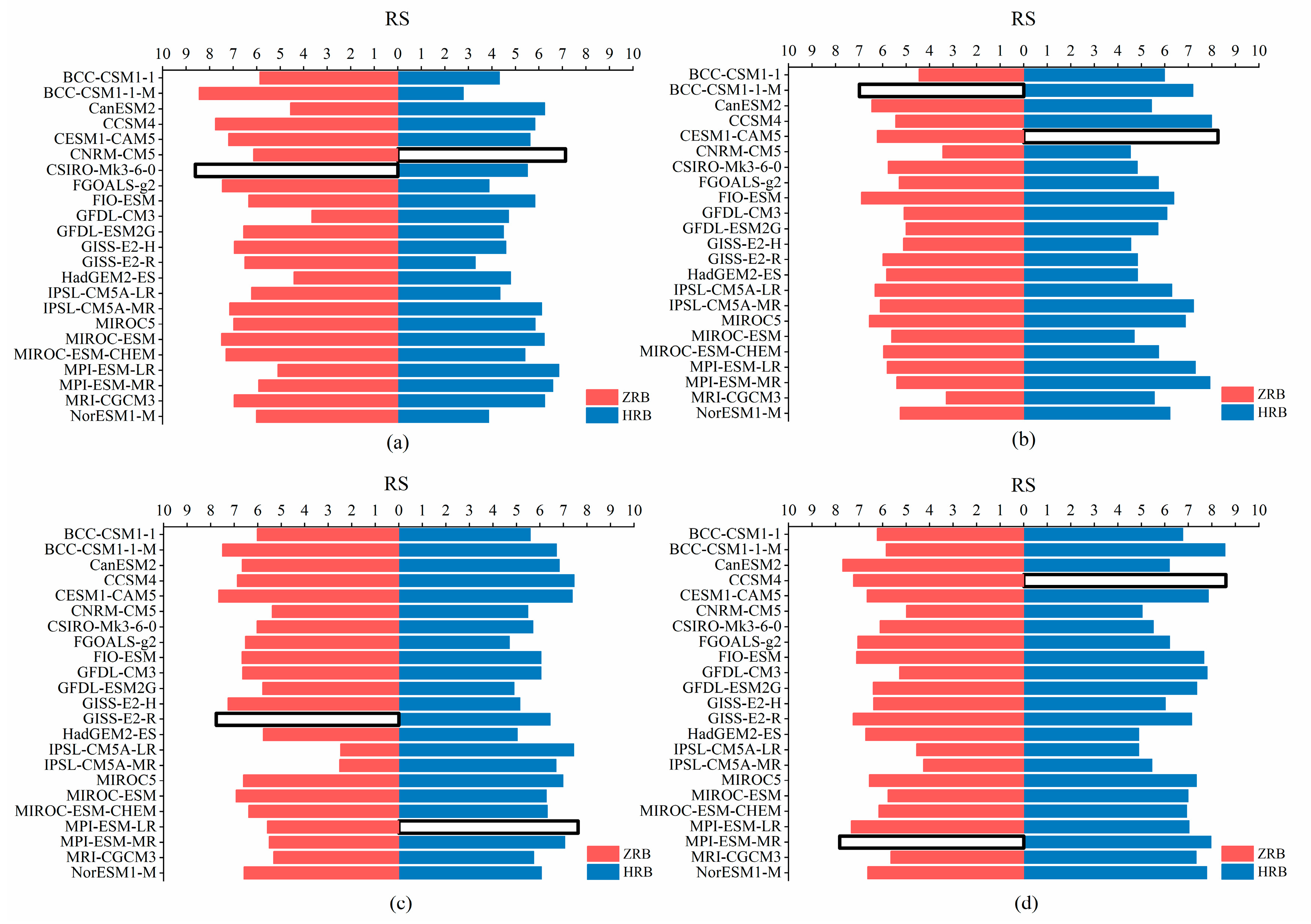
Figure 2 presents the comprehensive RS results of 23 GCMs for precipitation, mean air temperature, maximum air temperature, and minimum air temperature in two regions. In the ZRB, the optimal model for precipitation was CSIRO-MIK3-6-0 (RS = 8.6). The preferred models for mean air temperature, maximum air temperature, and minimum air temperature were BCC-CSM1-1-M (RS = 7.0), GISS-E2-R (RS = 7.8), and MPI-ESM-MR (RS = 7.8), respectively. Compared with the different preferred GCMs for each climate variable in the HRB, i.e., CNRM-CM5 (RS = 7.13) for precipitation and CESM1-CAM5 (RS = 8.25), MPI-ESM-LR (RS = 7.62), and CCSM4 (RS = 8.6) for the mean, maximum, and minimum air temperature, respectively, the significantly different advantages and disadvantages of the individual GCMs in different climate regions are highlighted.

3.1.2. Sensitivity Analysis of the Multi-Criterion Score-Based Method

To investigate the sensitivity of different climate variables to the final rank, the average RS of each GCM was calculated by removing the score of each climate variable in turn. As shown in Figure 3a, in the ZRB, the variation patterns of the RS values for the 23 GCMs with a single climate variable removed were similar to the initial pattern, demonstrating that it is difficult to judge which variable had the dominant impact on GCM performance in the ZRB. Therefore, taking the average RS of four climate variables as the assessment basis, the five preferred GCMs in the ZRB were BCC-CSM1-1-M, CESM1-CAM5, GISS-E2-R, CCSM4, and FIO-ESM. Due to missing and unavailable daily data for GISS-E2-R, CCSM4, and FIO-ESM, they were substituted by three GCMs: MIROC5, CSIRO-MK3-6-0, and FGOALS-g2, respectively. In the HRB (Figure 3b), RS values were most sensitive to precipitation, so the preferred GCMs exhibiting the best precipitation performance were selected for future climate change projection: CNRM-CM5, MPI-ESM-LR, MPI-ESM-MR, MRI-CGCM3, and CanESM2.

3.2. Calibration and Validation of Downscaling Models

3.2.1. SDSM Model

The Heihe River Basin

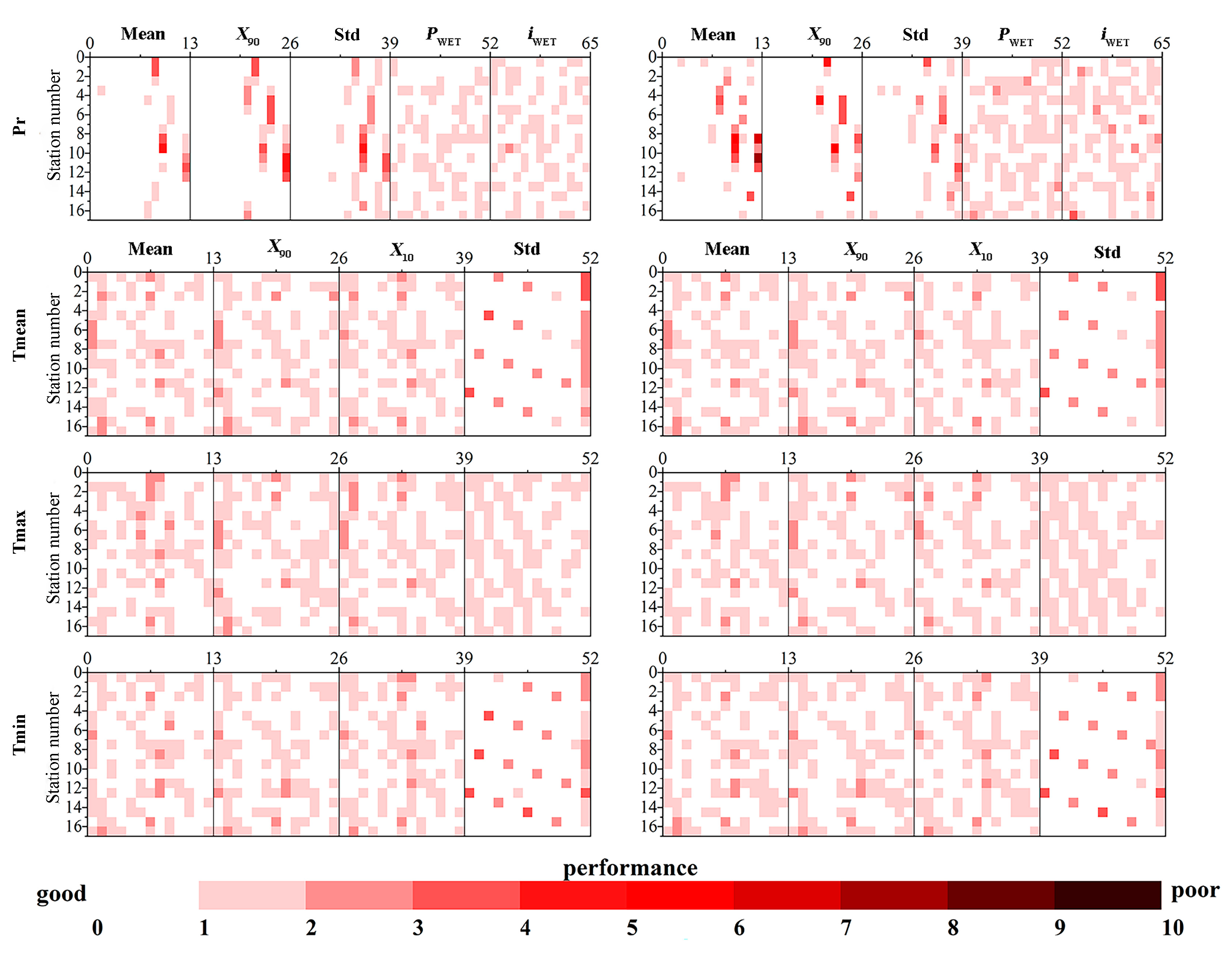
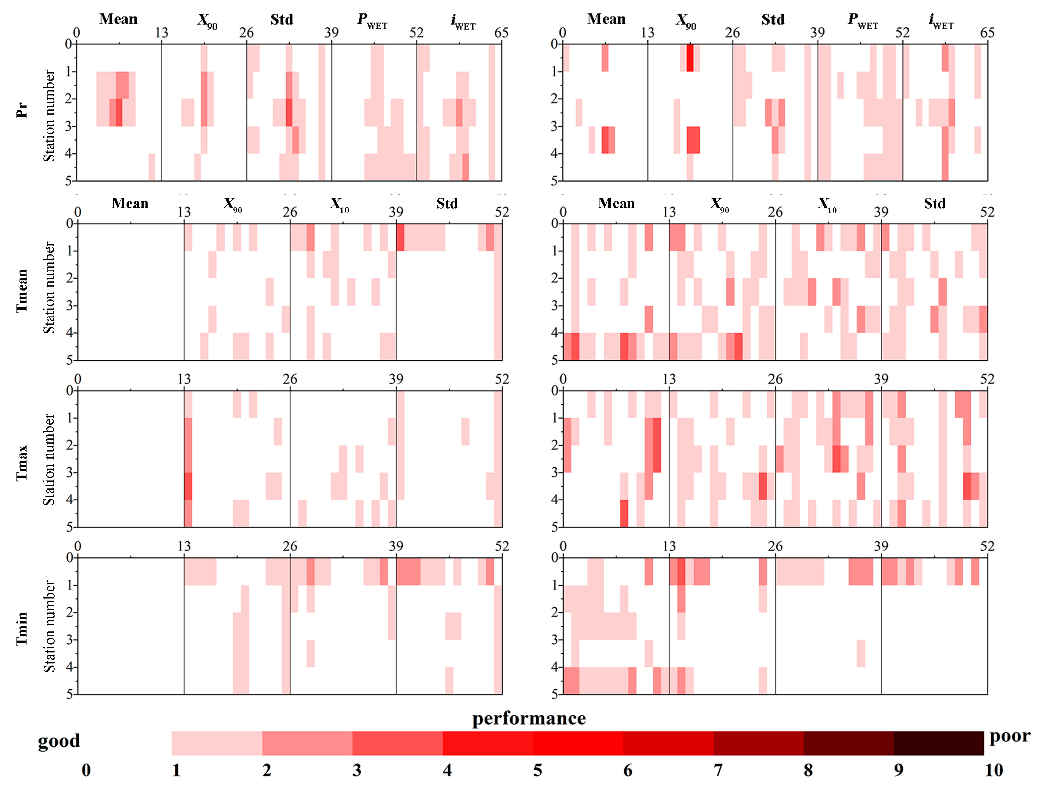
Figure 4 presents the standardized absolute errors in terms of evaluation indices for the observed and GCM data (the optimal model CNRM-CM5 was taken as the example here, the other four preferred models had similar performance), including four climate variables downscaled by SDSM during the calibration period (1961–1990, left) and validation period (1991–2000, right) in the HRB. The deeper the red color, the greater the absolute difference in model errors between the calibration and validation periods.

The results showed that the performance of SDSM constructed for the HRB was reasonable, and the simulation effect of precipitation was more accurate than that of air temperature. In detail, for precipitation, the simulation effect represented by P_WET and i_WET was basically within the lower error range in the two periods, which could be explained by the SDSM internal mechanism based on the coupling principle of multiple linear regression and the stochastic weather generator [22]. However, in the middle and lower reaches of the HRB, SDSM did not play a main role due to the arid climate with rare precipitation and sparse hydrological stations, complicating the capturing of the main climatic predictands and the establishment of an appropriate linear regression relationship. The findings of a previous study indicated that the extreme natural variability (time and space) of desert climates will increase the uncertainty of climate change modeling in arid regions [11]. For air temperature, the simulation effect indicated by the Mean, X₉₀, and X₁₀ showed that the biases of the three variables were similarly removed in most months, while the maximum air temperature and minimum air temperature exhibited better performance from the perspective of the standard deviation.

The Zhanghe River Basin

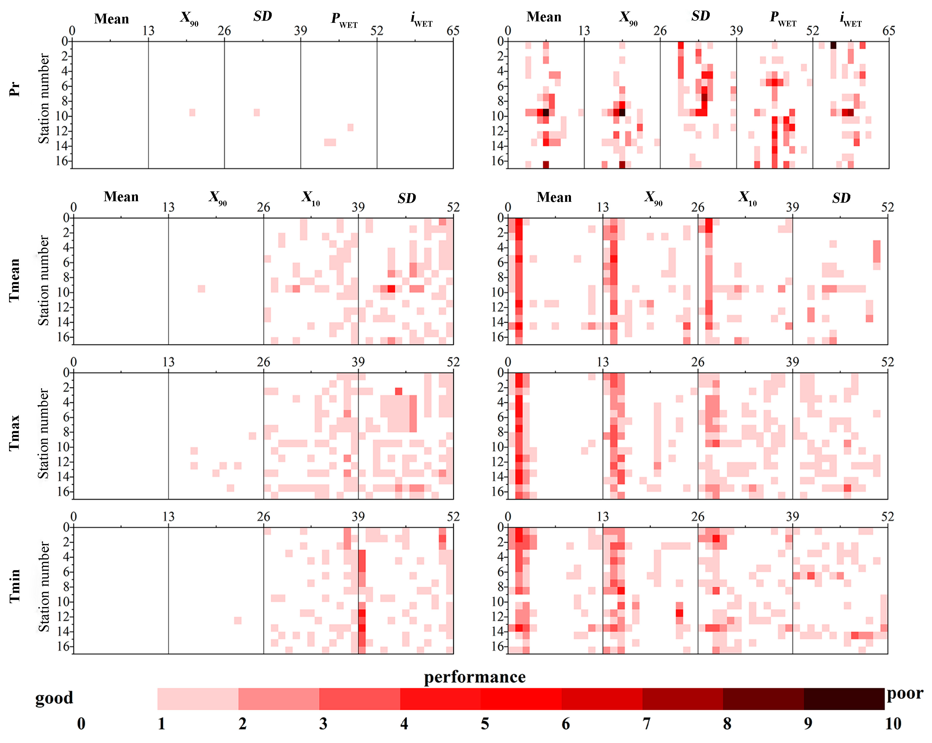
Figure 5 shows the evaluation results of precipitation performed similarly overall in the validation and calibration periods. We found that all the evaluation indices on the annual daily scale were appropriately corrected, while the simulation errors were mainly concentrated in the period from June to August. Regarding the three air temperature variables, the SDSM eliminated the biases of the mean value during the calibration period; however, slight biases remained during the validation period. For mean and maximum air temperature, the absolute errors of the X₉₀, X₁₀, and SD increased in the validation period. Considering the limited area of the ZRB, most meteorological stations used in this study were outside of the basin, not exactly matching the corresponding gridded data of the predictors from GCMs, which hindered the construction of the SDSM.

3.2.2. MOS Model

The Heihe River Basin

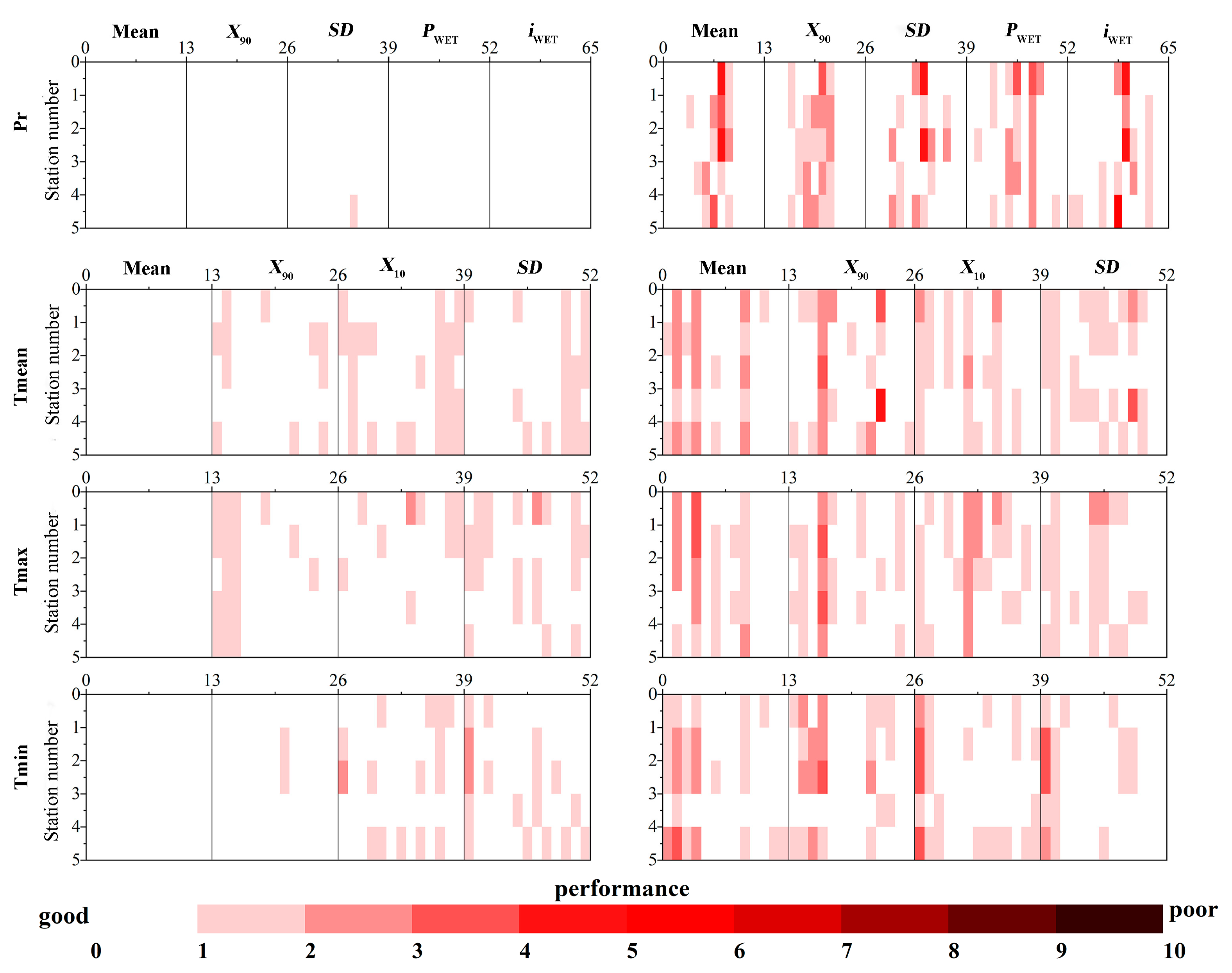
The CNRM-CM5, which exhibited the best performance in the HRB, is used for illustration. Figure 6 presents the evaluation indices for the observed and GCM data, including four climate variables downscaled by MOS for the calibration period (1961–1990, left) and validation period (1991–2005, right) in the HRB.

In terms of precipitation, the performance of MOS was excellent, as indicated by all five evaluation indices during the calibration period, while it performed slightly worse during the validation period due to the poor simulation effect (labeled using the darkest red) from June to August. However, the X₉₀ of precipitation in most months was zero in the HRB, due to its arid climate, which severely restricts the ability of the MOS model to capture the probability distribution of the climate variables. We further revealed that hidden nonlinear and complex factors, such as natural climate variability, inevitably affected the simulation effect.

The air temperature variables were accurately simulated, as demonstrated by the results of the Mean and X₉₀ in the calibration periods. During the validation period, there were relatively larger biases, mainly concentrated in the period from January to March, indicating that the DT method of MOS might be not suitable for bias correction of GCMs in regions with a large diurnal temperature range, such as the HRB, located in the inland arid region of northwestern China.

Figure 7 presents the performance of the evaluation indices for the observed and GCM data including four climate variables downscaled by MOS during the calibration period (1961–1990, left) and validation period (1991–2006, right) in the ZRB. Similarly, the results driven by the optimal model of BCC-CSM1-1-M are displayed for demonstration.

In terms of precipitation, all five types of evaluation indices indicated excellent simulation performance during the calibration period and a relative poorer but acceptable performance during the validation period. Compared with the performance in the arid HRB, the MOS method, which is based on distribution mapping, showed significant superiority in simulating precipitation in the ZRB, which has a relatively humid climate. This result is consistent with those of previous studies [65,76].

For the three temperature variables, the biases of the four evaluation indices, especially the mean index, were basically removed in the calibration period. Per the SD index, the simulation effect of the minimum air temperature was more accurate than that of the mean and maximum air temperature. This finding could be related to the subtropical humid climate of the ZRB, where the annual maximum air temperature changes dramatically, resulting in difficulty in capturing the regular variation pattern.

3.3. Optimization Assessment of SDSM and MOS for the Two Basins

3.3.1. Assessment of the HRB

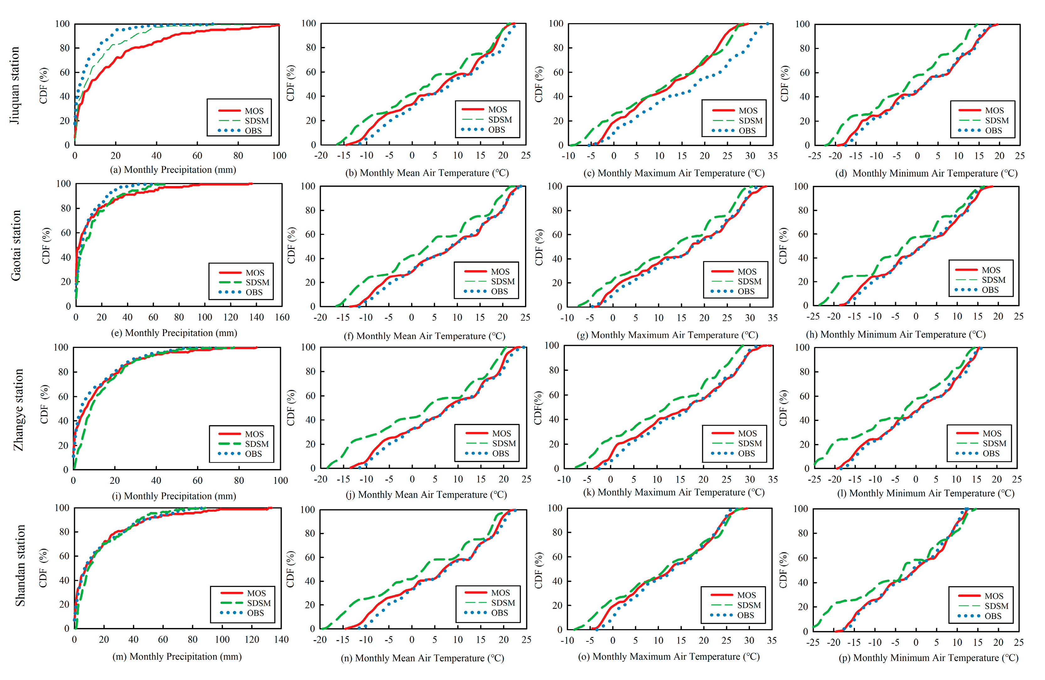
Cumulative distribution functions (CDFs) of the annual precipitation and mean, maximum, and minimum air temperature were built to compare the differences between SDSM and MOS for the period of 1991–2005 based on the simulation results of four monitoring stations (Jiuquan, Gaotai, Zhangye, and Shandan) located in the middle irrigated region of the HRB. As shown in Figure 8, both CDF curves representing the distribution characteristics of precipitation simulated by the two methods were similar to those of the observed data, with a consistent overestimation of precipitation. The observed monthly precipitation ranged between 0 and 80 mm, while the range of precipitation simulated by MOS exceeded 100 mm for each station. Compared with MOS, the results simulated by SDSM were relatively closer to the CDF curve of the observed data. In addition, precipitation extremes simulated by MOS were much larger than the observed values.

In terms of air temperature, the SDSM underestimated the three temperature variables of each station, and its simulation of the minimum and mean air temperatures at the Shandan and Zhangye stations was more distributed in the lower temperature range. For maximum air temperature, except for the simulation effect of the Shandan station, the value distribution of the other stations as shifted to the left compared with the measured data, that is, the overall variation range of maximum air temperature decreased. In contrast to the SDSM model, the MOS model more accurately simulated the distribution of the three air temperature variables, only underestimating the larger value area of the maximum air temperature at Jiuquan Station.

Accurate simulation of regional precipitation has long remained a challenge in downscaling [77,78,79]. Hence, one essential criterion by which to judge the suitability of a downscaling model for a certain region is whether the model can capture precipitation characteristics. For the HRB, although the simulation of air temperature variables by SDSM was inferior to that of MOS, which was still acceptable, SDSM was found to be the more suitable downscaling model for the HRB due to its more accurate precipitation simulation.

3.3.2. Assessment in the ZRB

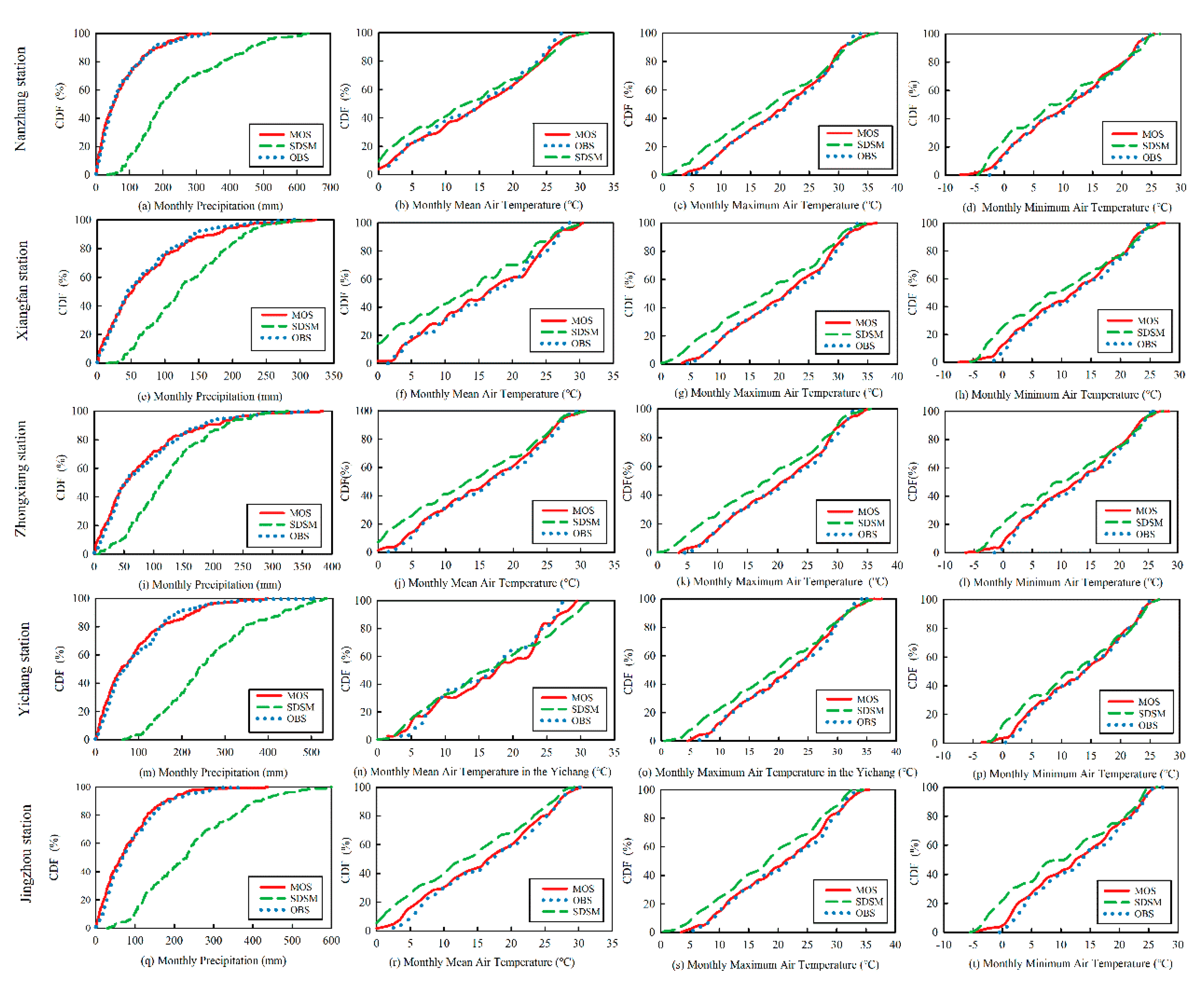
Based on the observed and simulated data from the five gauging stations (Nanzhang, Xiangfan, Zhongxiang, Yichang, and Jingzhou), the CDFs of the annual precipitation and mean, maximum, and minimum air temperature were built during the period of 1991–2006. As shown in Figure 9, the performance of the precipitation distribution characteristics simulated by MOS was much better than that of SDSM, which was consistent with the CDF of the observed data. However, the SDSM model significantly overestimated the frequency of precipitation extremes. For example, the observed annual monthly precipitation was within 200 mm for the Nanzhang, Yichang, and Jingzhou stations, with relatively higher annual precipitation, while the values simulated by SDSM almost reached 500 mm for these three stations.

In terms of air temperature simulation results, the SDSM model underestimated the values of the three air temperature variables at each station. Different from the HRB, the distribution characteristics of the mean, maximum, and minimum air temperature were underestimated in the higher temperature zone, indicating that the distribution of monthly air temperature in the ZRB simulated by SDSM was lower than the observed data. For MOS, the simulation performance was excellent from both the perspective of the overall range and cumulative frequency of different intervals.

Overall, compared with the performance of SDSM in the ZRB, the precipitation and air temperature simulated by MOS were more accurate, so MOS was determined to be a suitable downscaling model for future climate change projection in the ZRB.

3.4. Climate Change Projections

Results for the HRB were projected in the study by Wang et al. [31]; the results for the ZRB are presented here for illustration.

3.4.1. Precipitation Scenarios

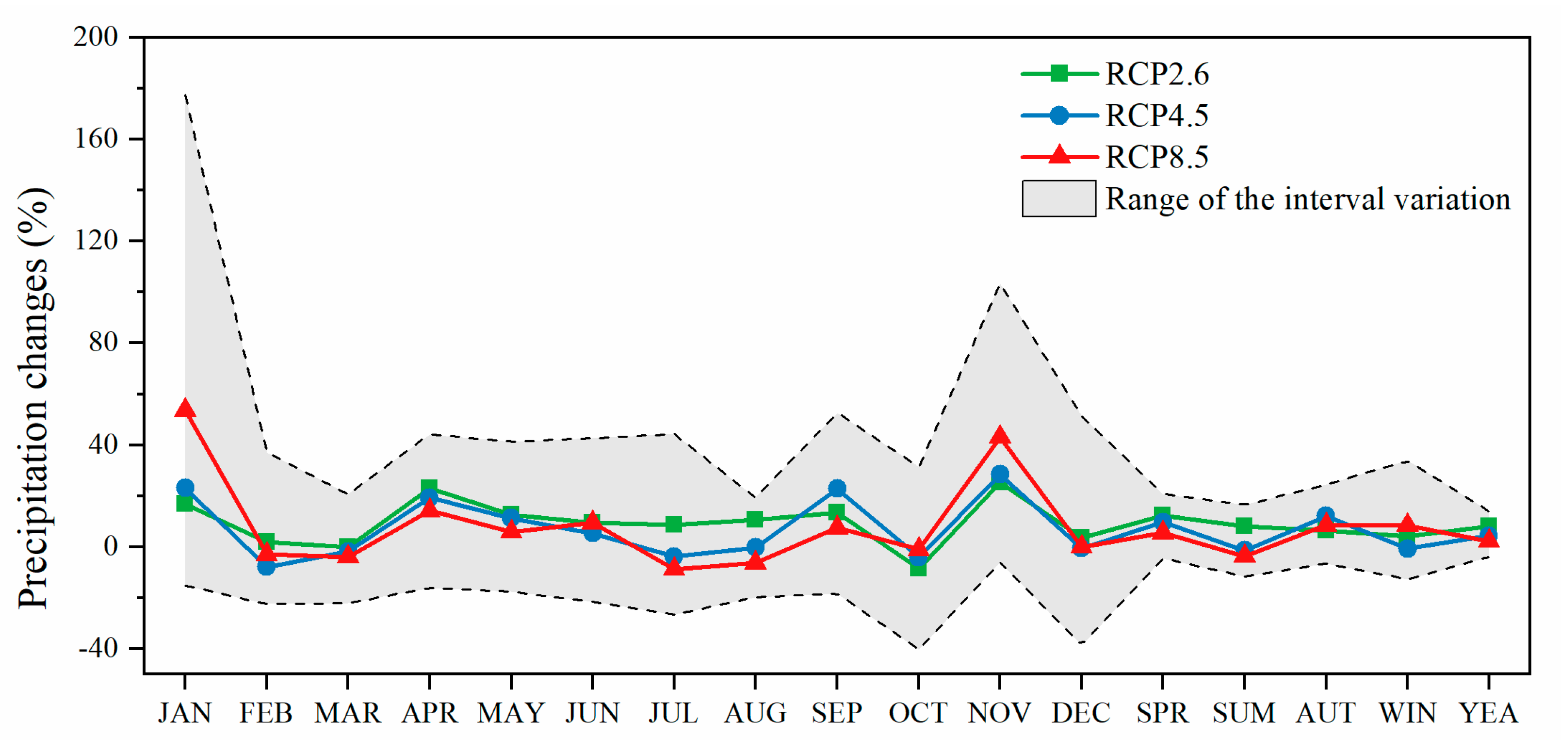
The five optimal GCMs were used to project the precipitation in the ZRB under the RCP2.6, RCP4.5, and RCP8.5 scenarios based on the constructed MOS model. Future changes in precipitation were analyzed based on the differences between the baseline period (1991–2006) and a future period (2021–2050). Figure 10 depicts the temporal variation patterns of precipitation at monthly, seasonal, and annual scales. Mean annual precipitation projected by multi-GCMs under most scenarios showed an increasing trend, ranging from −3.9% to +13.8%. At the seasonal scale, the changes were most obvious in autumn and winter, with significant fluctuations, whereas changes in precipitation in spring and summer varied between −10% and +20%. At the monthly scale, most changes in the future under different scenarios ranged from −20% to +45%. The largest increase occurred in January when simulated by FGOALS-g2 under the RCP8.5 scenario, reaching 177.5%, whereas the largest decline occurred in October, also simulated by FGOALS-g2 under the RCP 2.6 scenario, at a rate of 40.3%. The simulation results under the RCP2.6 scenario at various temporal scales all presented an increasing trend, with the highest increase in November, whereas the simultaneous changes under the RCP8.5 scenario were relatively smaller.

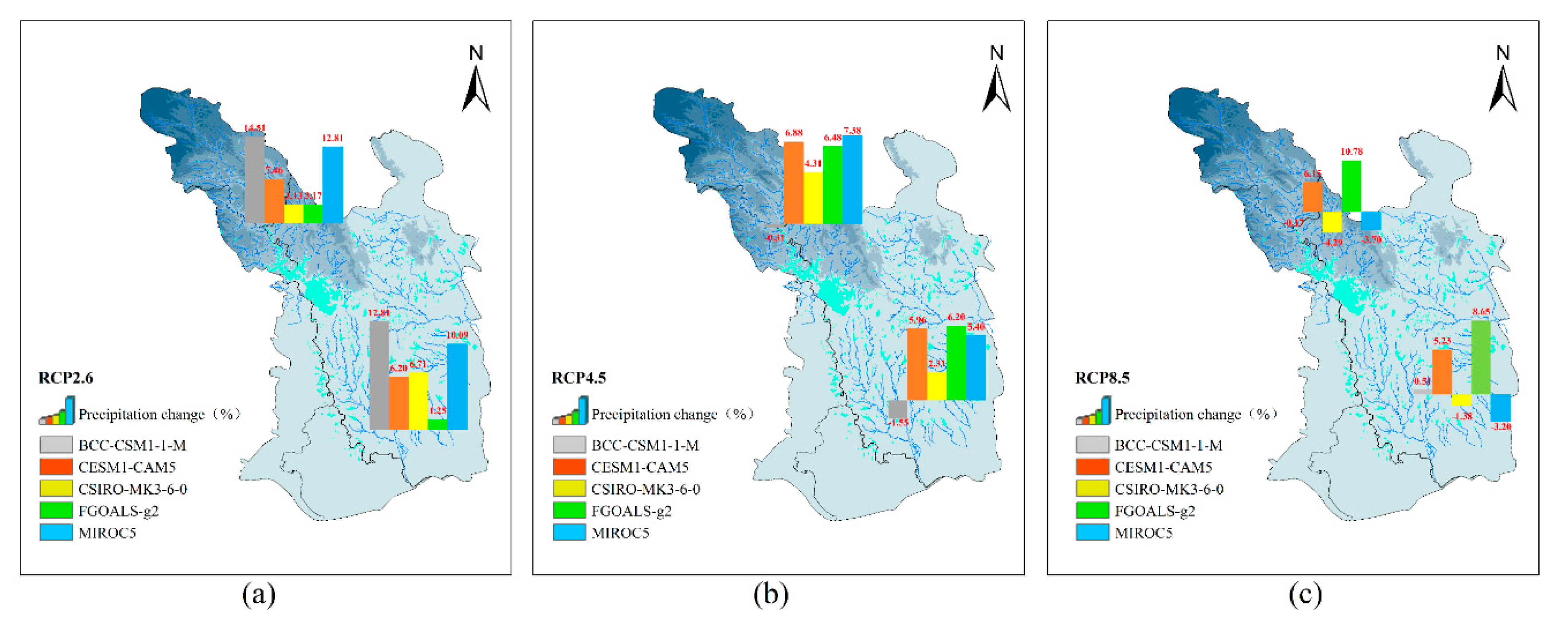
Spatial variations in precipitation in the upper and lower reaches of the Zhanghe River Basin under the three RCPs are shown in Figure 11. The mean annual precipitation under the RCP2.6 and RCP4.5 scenarios showed an increasing trend, and the increase in the upstream area was slightly higher than that in the downstream. Under the RCP8.5 scenario, except for FGOALS-g2, the precipitation projected by the other four GCMs either showed a decreasing trend or a slight increasing trend. Overall, the projected changes in precipitation in the HRB during 2021–2050 ranged from −4.29% to +14.51% and from −3.2% to +12.81% in the upstream and downstream regions, respectively. With the increase in CO₂ concentration defined in the RCPs, i.e., RCP8.5 > RCP4.5 > RCP2.6, the increases in precipitation projected by CESM1-CAM5, MIROC5, and CSIRO-MK3-6-0 gradually decreased, whereas an opposite changing pattern was projected by FGOALS-g2. We found no consistent variation in precipitation with the rising CO₂ concentration projected by BCC-CSM1-1-M, showing a significant increase under RCP2.6 with a rate of 14.5% in the upstream and 12.8% in the downstream areas, and a smaller change ranging from −1.55% to +0.51% in the whole basin under RCP4.5 and RCP8.5.

3.4.2. Maximum Air Temperature Scenarios

As shown in Figure 12, the changes in maximum air temperature projected by multi-GCMs under the three RCP scenarios in the ZRB at different time scales mostly exhibited an increasing trend, ranging from 0.5 to 2.5 °C. The increases in maximum air temperature projected by BCC-CSM1-1-M were mainly located in the upper-value region of the variation ranges, while changes projected by FGOALS-g2 were distributed in the lower-value region of the variation ranges. At the seasonal scale, projected increases mainly occurred in summer, ranging between 0.4 and 2.4 °C, and in winter, ranging between 0.6 and 2.5 °C. The increases in annual maximum air temperature projected by the multi-GCMs under the three RCP scenarios were all higher than 1 °C.

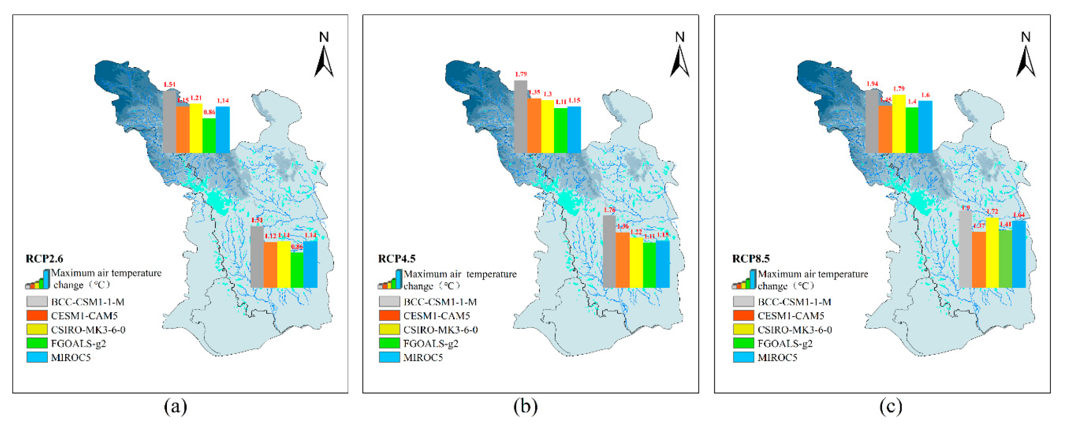
In Figure 13, the mean annual maximum air temperature projected by all GCMs under the three RCP scenarios demonstrated a consistent warming trend throughout the whole basin, and the increasing rates gradually amplified as the CO₂ emission concentration increased. However, the increases in different regions exhibited visible differences. Compared with changes projected by the same GCM under different RCP scenarios, the maximum air temperature projected by BCC-CSM1-1-M under RCP8.5 increased most significantly, i.e., 1.94 °C in the upstream and 1.9 °C in the downstream region. The lowest increase was projected by FGOALS-g2 under RCP2.6 in the downstream, i.e., 0.86 °C. Compared with the increases in the lower reaches ranging from 0.86 to 1.9 °C, the increases in the upper reaches projected by the five preferred GCMs under the three RCP scenarios were slightly larger, ranging from 0.86 to 1.94 °C.

3.4.3. Minimum Air Temperature Scenarios

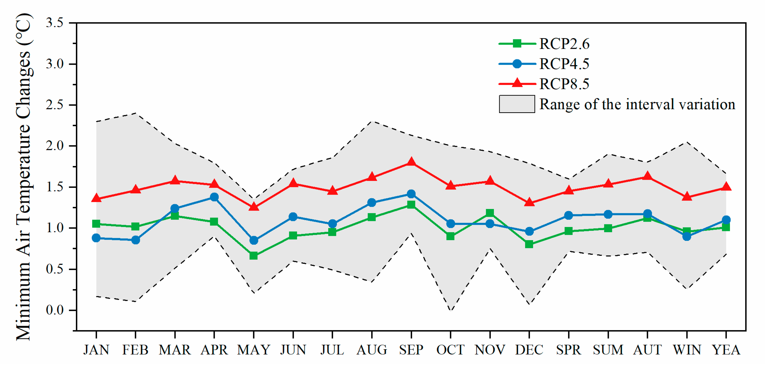
The minimum air temperature simulated by different GCMs also exhibited an increasing trend under all three RCP scenarios at different time scales (Figure 14), consistent with the temporal variations in the maximum air temperature. The minimum air temperature simulated by the five preferred GCMs under RCP8.5 mostly contributed to the upper limits of the variation ranges at different time scales, with a maximum increase of 2.4 °C, while the changes projected by the five GCMs under RCP2.6 and RCP4.5 fluctuated between the upper and lower limit values of the variation ranges. In terms of changes at the seasonal scale, the increase in minimum air temperature mainly ranged from 0.5 to 2.0 °C, i.e., slightly less than that of the maximum air temperature. The maximum fluctuation occurred in winter, varying between 0.3 and 2.0 °C, while the increase in the mean annual minimum air temperature ranged between 0.7 and 1.7 °C.

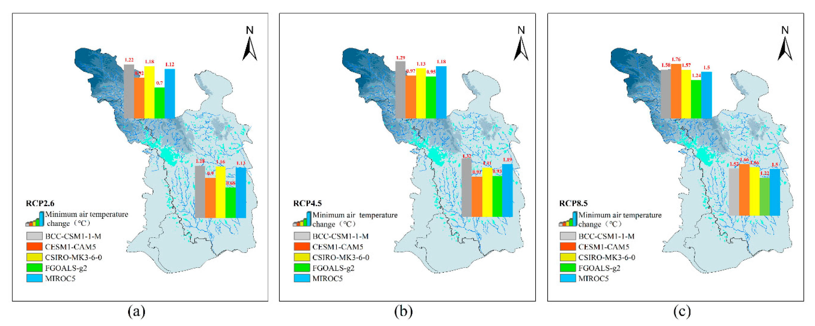
Similar to the maximum air temperature, the minimum air temperature exhibited a consistent warming trend throughout the whole basin (Figure 15), and the increasing rates gradually amplified as the CO₂ emission concentration increased. However, the increases showed spatial differences in the upper and lower reaches. CSIRO-MK3-6-0, under the RCP8.5 scenario over the whole basin, projected the most obvious increase, i.e., 1.76 °C in the upstream and 1.66 °C in the downstream region. The lowest increase was projected by FGOALS-g2 under RCP 2.6 in the downstream region, i.e., 0.68 °C. Compared with the increases in the lower reaches ranging from 0.68 to 1.66 °C, the increases in the upper reaches projected by the five preferred GCMs under the three RCP scenarios were slightly higher, ranging from 0.7 to 1.76 °C. Although increases in both maximum and minimum air temperatures in the upper reaches projected under the three scenarios were larger than those in the lower reaches, the increases in the maximum air temperature were more significant compared with those of the minimum air temperature.

4. Conclusions

In this study, to explore the influences of multi-GCMs and different downscaling methods on climate change projection in various climate zones in detail, the Heihe River Basin, located in northwestern China, and the Zhanghe River Basin, located in the lower reaches of the Yangtze River Basin, were selected to represent the north–south discrepancy in climate in China. Our conclusions are summarized as follows:

(1)

According to the results of the score-based method and sensitivity analysis, five optimal GCMs were selected for each basin: CNRM-CM5, MPI-ESM-LR, MPI-ESM-MR, MRI-CGCM3, and CANESM2 were suitable for the HRB (arid climate) in North China; BCC-CSM1-1-M, CESM1-CAM5, MIROC5, CSIRO-MK3-6-0, and FGOALS-g2 were more appropriate for the ZRB (humid climate) in South China.

(2)

For different climate variables, SDSM and MOS showed superiority in different climatic basins. In the HRB, the performance of SDSM in downscaling precipitation was better than that of MOS, whereas MOS performed better in downscaling the temperature variables. In the ZRB, for both precipitation and temperature, MOS performed better than SDSM.

(3)

As indicated by the cumulative distribution functions (CDFs), MOS better captured the precipitation distribution characteristics in the humid region, but not in the arid region, implying that the climate characteristics of a specific region significantly impact the selection of the downscaling method, which is critical to the reliability of future climate change projections.

(4)

In the HRB, which is characterized as an inland arid climate, the multi-GCM-projected mean annual precipitation under the three RCP scenarios showed a decreasing trend, ranging between −12.3% and 4.4%. The most significant decrease appeared in the upstream [33]. In the ZRB, located in the middle reaches of the Yangtze River, the projected mean annual precipitation mostly exhibited an upward tendency ranging between −3.9% and 13.8%. The air temperature was projected to consistently increase in the HRB and ZRB, and the increase in the maximum air temperature was slightly larger than that of the minimum air temperature.

The specific suggestions inferred from this study include: (1) Considering the use of available observations as much as possible. In this study, ERA-40 reanalysis data starting in 1961 was used instead of ERA-Interim, which were of superior quality starting in 1979, which might be helpful for the calibration of statistical downscaling models. (2) With the release of Phase 6 of the Coupled Model Inter-comparison Project (CMIP6), a further study will be conducted to explore the superiority of the latest model outputs and provide more reliable and accurate prediction results for regional future climate change prediction using a variety of downscaling technologies. The climate change projection framework developed and recommended in this study for the north and south of China provides scientific support for sustainable water resource management subject to climate change.

References

- Chen, J.; Xu, C.; Guo, S.; Chen, H. Progress and challenge in statistically downscaling climate model outputs. J. Water Resour. Res. 2016, 5, 299–313. [Google Scholar] [CrossRef]
- Gooré Bi, E.; Gachon, P.; Vrac, M.; Monette, F. Which downscaled rainfall data for climate change impact studies in urban areas? Review of current approaches and trends. Theor. Appl. Climatol. 2017, 127, 685–699. [Google Scholar] [CrossRef]
- Tong, S.; Berry, H.L.; Ebi, K.; Bambrick, H.; Hu, W.; Green, D.; Hanna, E.; Wang, Z.; Butler, C.D. Climate change, food, water and population health in China. B. World Health Organ. 2016, 94, 759–765. [Google Scholar] [CrossRef] [PubMed]
- Xu, Z.; Liu, L.; Yang, X. Study on extreme climate events and drought/flood disasters: Review and prospect. China Flood Drought Manag. 2017, 27, 66–74. [Google Scholar]
- Fang, G.H.; Yang, J.; Chen, Y.N.; Zammit, C. Comparing bias correction methods in downscaling meteorological variables for a hydrologic impact study in an arid area in China. Hydrol. Earth Syst. Sci. 2015, 19, 2547–2559. [Google Scholar] [CrossRef] [Green Version]
- Wang, L.; Ranasinghe, R.; Maskey, S.; van Gelder, P.H.A.J.; Vrijling, J.K. Comparison of empirical statistical methods for downscaling daily climate projections from CMIP5 GCMs: A case study of the Huai River Basin, China. Int. J. Climatol. 2016, 36, 145–164. [Google Scholar] [CrossRef]
- Yang, Y.; Tang, J.; Xiong, Z.; Wang, S.; Yuan, J. An intercomparison of multiple statistical downscaling methods for daily precipitation and temperature over China: Present climate evaluations. Clim. Dynam. 2019, 53, 4629–4649. [Google Scholar] [CrossRef]
- Dai, A.; Rasmussen, R.M.; Ikeda, K.; Liu, C. A new approach to construct representative future forcing data for dynamic downscaling. Clim. Dynam. 2020, 55, 315–323. [Google Scholar] [CrossRef]
- Mascaro, G.; Viola, F.; Deidda, R. Evaluation of Precipitation from EURO-CORDEX Regional Climate Simulations in a Small-Scale Mediterranean Site. J. Geophys. Res. Atmos. 2018, 123, 1604–1625. [Google Scholar] [CrossRef]
- Zou, L.; Zhou, T.; Peng, D. Dynamical downscaling of historical climate over CORDEX East Asia domain: A Comparison of regional ocean-atmosphere coupled model to stand-alone RCM simulations. J. Geophys. Res. Atmos. 2016, 121, 1442–1458. [Google Scholar] [CrossRef] [Green Version]
- Teutschbein, C.; Seibert, J. Is bias correction of regional climate model (RCM) simulations possible for non-stationary conditions? Hydrol. Earth Syst. Sci. 2013, 17, 5061–5077. [Google Scholar] [CrossRef] [Green Version]
- Suzuki-Parker, A.; Kusaka, H.; Takayabu, I.; Dairaku, K.; Ishizaki, N.N.; Ham, S. Contributions of GCM/RCM Uncertainty in Ensemble Dynamical Downscaling for Precipitation in East Asian Summer Monsoon Season. Sola 2018, 14, 97–104. [Google Scholar] [CrossRef]
- Abiodun, B.J.; Omar, S.A.; Lennard, C.; Jack, C. Using regional climate models to simulate extreme rainfall events in the Western Cape, South Africa. Int. J. Climatol. 2016, 36, 689–705. [Google Scholar] [CrossRef]
- Cao, X.; Tang, R.; Wang, W.; Xue, J. Precipitation projection of the Luanhe River Basin based on two statistical downscaling models. J. Yangzhou Univ. (Nat. Sci. Ed.) 2016, 19, 28–32. [Google Scholar]
- Fan, L.; Fu, C.; Chen, D. Estimation of local temperature change scenarios in North China using statistical downscaling method. Chin. J. Atmos. Sci. 2007, 31, 887–897. [Google Scholar]
- Liu, Y.; Guo, W.; Feng, J.; Zhang, K. A summary of methods for statistical downscaling of meteorological data. Adv. Earth Sci. 2011, 26, 837–847. [Google Scholar]
- Stennett-Brown, R.K.; Jones, J.J.P.; Stephenson, T.S.; Taylor, M.A. Future Caribbean temperature and rainfall extremes from statistical downscaling. Int. J. Climatol. 2017, 37, 4828–4845. [Google Scholar] [CrossRef]
- Tang, J.; Niu, X.; Wang, S.; Gao, H.; Wang, X.; Wu, J. Statistical downscaling and dynamical downscaling of regional climate in China: Present climate evaluations and future climate projections. J. Geophys. Res. Atmos. 2016, 121, 2110–2129. [Google Scholar] [CrossRef] [Green Version]
- Chiew, F.H.S.; Kirono, D.G.C.; Kent, D.M.; Frost, A.J.; Charles, S.P.; Timbal, B.; Nguyen, K.C.; Fu, G. Comparison of runoff modelled using rainfall from different downscaling methods for historical and future climates. J. Hydrol. 2010, 387, 10–23. [Google Scholar] [CrossRef]
- Cheng, C.S.; Auld, H.; Li, Q.; Li, G. Possible impacts of climate change on extreme weather events at local scale in south-central Canada. Clim. Chang. 2012, 112, 963–979. [Google Scholar] [CrossRef] [Green Version]
- Sunyer, M.A.; Hundecha, Y.; Lawrence, D.; Madsen, H.; Willems, P.; Martinkova, M.; Vormoor, K.; Bürger, G.; Hanel, M.; Kriaučiūnienė, J.; et al. Inter-comparison of statistical downscaling methods for projection of extreme precipitation in Europe. Hydrol. Earth Syst. Sci. 2015, 19, 1827–1847. [Google Scholar] [CrossRef] [Green Version]
- Liu, Z.; Xu, Z.; Charles, S.P.; Fu, G.; Liu, L. Evaluation of two statistical downscaling models for daily precipitation over an arid basin in China. Int. J. Climatol. 2011, 31, 2006–2020. [Google Scholar] [CrossRef]
- Hu, Y.; Maskey, S.; Uhlenbrook, S. Downscaling daily precipitation over the Yellow River source region in China: A comparison of three statistical downscaling methods. Theor. Appl. Climatol. 2013, 112, 447–460. [Google Scholar] [CrossRef]
- Huang, J.; Zhang, J.; Zhang, Z.; Xu, C.; Wang, B.; Yao, J. Estimation of future precipitation change in the Yangtze River basin by using statistical downscaling method. Stoch. Env. Res. Risk Assess. 2011, 25, 781–792. [Google Scholar] [CrossRef]
- Liu, W.; Fu, G.; Liu, C.; Charles, S.P. A comparison of three multi-site statistical downscaling models for daily rainfall in the North China Plain. Theor. Appl. Climatol. 2013, 111, 585–600. [Google Scholar] [CrossRef]
- Rana, A.; Moradkhani, H. Spatial, temporal and frequency based climate change assessment in Columbia River Basin using multi downscaled-scenarios. Clim. Dynam. 2016, 47, 579–600. [Google Scholar] [CrossRef]
- San-Martín, D.; Manzanas, R.; Brands, S.; Herrera, S.; Gutiérrez, J.M. Reassessing model uncertainty for regional projections of precipitation with an ensemble of statistical downscaling methods. J. Clim. 2017, 30, 203–223. [Google Scholar] [CrossRef]
- Zelazowski, P.; Huntingford, C.; Mercado, L.M.; Schaller, N. Climate pattern-scaling set for an ensemble of 22 GCMs—Adding uncertainty to the IMOGEN version 2.0 impact system. Geosci. Model. Dev. 2018, 11, 541–560. [Google Scholar] [CrossRef] [Green Version]
- Kusangaya, S.; Warburton Toucher, M.L.; van Garderen, E.A. Evaluation of uncertainty in capturing the spatial variability and magnitudes of extreme hydrological events for the uMngeni catchment, South Africa. J. Hydrol. 2018, 557, 931–946. [Google Scholar] [CrossRef]
- Tegegne, G.; Melesse, A.M.; Worqlul, A.W. Development of multi-model ensemble approach for enhanced assessment of impacts of climate change on climate extremes. Sci. Total Environ. Sci. 2020, 704, 135357. [Google Scholar] [CrossRef]
- Das, L.; Dutta, M.; Mezghani, A.; Benestad, R.E. Use of observed temperature statistics in ranking CMIP5 model performance over the Western Himalayan Region of India. Int. J. Climatol. 2018, 38, 554–570. [Google Scholar] [CrossRef]
- Li, X.; Zhang, K.; Babovic, V. Projections of Future Climate Change in Singapore Based on a Multi-Site Multivariate Downscaling Approach. Water 2019, 11, 2300. [Google Scholar] [CrossRef] [Green Version]
- Wang, R.; Cheng, Q.; Liu, L.; Yan, C.; Huang, G. Multi-model projections of climate change in different RCP scenarios in an arid inland region, Northwest China. Water 2019, 11, 347. [Google Scholar] [CrossRef] [Green Version]
- Fu, G.; Liu, Z.; Charles, S.P.; Xu, Z.; Yao, Z. A score-based method for assessing the performance of GCMs: A case study of southeastern Australia. J. Geophysi. Res. Atmos. 2013, 118, 4154–4167. [Google Scholar] [CrossRef]
- Li, F.; Xu, Z.; Liu, X.; Li, X.; Liu, Z. Assessment on performance of different general circulation models in Songhuajiang River basin. Hydrology 2011, 31, 24–31. [Google Scholar]
- Liu, L.; Guo, Z.; Huang, G.; Wang, R. Water productivity evaluation under multi-GCM projections of climate change in oases of the Heihe River basin, northwest China. Int. J. Environ. Res. Public Health 2019, 16, 1706. [Google Scholar] [CrossRef] [Green Version]
- Zhang, A.; Zheng, C.; Wang, S.; Yao, Y. Analysis of streamflow variations in the Heihe River Basin, northwest China: Trends, abrupt changes, driving factors and ecological influences. J. Hydrol. Reg. Stud. 2015, 3, 106–124. [Google Scholar] [CrossRef] [Green Version]
- Dee, D.P.; Uppala, S.M.; Simmons, A.J.; Berrisford, P.; Poli, P.; Kobayashi, S.; Andrae, U.; Balmaseda, M.A.; Balsamo, G.; Bauer, P.; et al. The ERA-Interim reanalysis: Configuration and performance of the data assimilation system. Q. J. Roy. Meteor. Soc. 2011, 137, 553–597. [Google Scholar] [CrossRef]
- Chen, J.; St-Denis, B.G.; Brissette, F.P.; Lucas-Picher, P. Using Natural Variability as a Baseline to Evaluate the Performance of Bias Correction Methods in Hydrological Climate Change Impact Studies. J. Hydrometeorol. 2016, 17, 2155–2174. [Google Scholar] [CrossRef]
- Shu, Q.; Wang, Q.; Song, Z.; Qiao, F.; Zhao, J.; Chu, M.; Li, X. Assessment of Sea Ice Extent in CMIP6 with Comparison to Observations and CMIP5. Geophys. Res. Lett. 2020, 47, e2020GL087965. [Google Scholar] [CrossRef]
- Kudo, R.; Yoshida, T.; Masumoto, T. Uncertainty analysis of impacts of climate change on snow processes: Case study of interactions of GCM uncertainty and an impact model. J. Hydrol. 2017, 548, 196–207. [Google Scholar] [CrossRef]
- Rosenberg, E.A.; Keys, P.W.; Booth, D.B.; Hartley, D.; Burkey, J.; Steinemann, A.C.; Lettenmaier, D.P. Precipitation extremes and the impacts of climate change on stormwater infrastructure in Washington State. Clim. Chang. 2010, 102, 319–349. [Google Scholar] [CrossRef] [Green Version]
- Vetter, T.; Reinhardt, J.; Floerke, M.; van Griensven, A.; Hattermann, F.; Huang, S.; Koch, H.; Pechlivanidis, I.G.; Ploetner, S.; Seidou, O.; et al. Evaluation of sources of uncertainty in projected hydrological changes under climate change in 12 large-scale river basins. Clim. Chang. 2017, 141, 419–433. [Google Scholar] [CrossRef]
- Liu, W.; Xu, Z.; Li, F.; Qiu, L. GCM performance on simulating climatological factors in Yarlung Zangbo river basin based on a ranked score method. J. Beijing Normal Univ. (Nat. Sci.) 2013, 49, 304–311. [Google Scholar]
- Boehnisch, A.; Ludwig, R.; Leduc, M. Using a nested single-model large ensemble to assess the internal variability of the North Atlantic Oscillation and its climatic implications for central Europe. Earth Syst. Dynam. 2020, 11, 617–640. [Google Scholar] [CrossRef]
- Borges, P.D.A.; Barfus, K.; Weiss, H.; Bernhofer, C. Extended predictor screening, application and added value of statistical downscaling of a CMIP5 ensemble for single-site projections in Distrito Federal, Brazil. Int. J. Climatol. 2017, 37, 46–65. [Google Scholar] [CrossRef]
- Xu, Z.X.; Takeuchi, K.; Ishidaira, H. Monotonic trend and step changes in Japanese precipitation. J. Hydrol. 2003, 279, 144–150. [Google Scholar] [CrossRef]
- Peng, S.; Ding, Y.; Wen, Z.; Chen, Y.; Cao, Y.; Ren, J. Spatiotemporal change and trend analysis of potential evapotranspiration over the Loess Plateau of China during 2011–2100. Agric. Forest Meteorol. 2017, 233, 183–194. [Google Scholar] [CrossRef] [Green Version]
- Mtongori, H.I.; Stordal, F.; Benestad, R.E. Evaluation of Empirical Statistical Downscaling Models’ Skill in Predicting Tanzanian Rainfall and Their Application in Providing Future Downscaled Scenarios. J. Clim. 2016, 29, 3231–3252. [Google Scholar] [CrossRef] [Green Version]
- Frazier, A.G.; Timm, O.E.; Giambelluca, T.W.; Diaz, H.F. The influence of ENSO, PDO and PNA on secular rainfall variations in Hawai’i. Clim. Dynam. 2018, 51, 2127–2140. [Google Scholar] [CrossRef]
- Perkins, S.E.; Pitman, A.J.; Holbrook, N.J.; McAneney, J. Evaluation of the AR4 climate models’ simulated daily maximum temperature, minimum temperature, and precipitation over Australia using probability density functions. J. Clim. 2007, 20, 4356–4376. [Google Scholar] [CrossRef]
- Wilby, R.L.; Dawson, C.W.; Barrow, E.M. SDSM—A decision support tool for the assessment of regional climate change impacts. Environ. Model. Softw. 2002, 17, 145–157. [Google Scholar] [CrossRef]
- Mullan, D.; Chen, J.; Zhang, X.J. Validation of non-stationary precipitation series for site-specific impact assessment: Comparison of two statistical downscaling techniques. Clim. Dynam. 2016, 46, 967–986. [Google Scholar] [CrossRef] [Green Version]
- Gebrechorkos, S.H.; Hülsmann, S.; Bernhofer, C. Statistically downscaled climate dataset for East Africa. Sci. Data 2019, 6, 1–8. [Google Scholar] [CrossRef] [Green Version]
- Tavakol-Davani, H.; Nasseri, M.; Zahraie, B. Improved statistical downscaling of daily precipitation using SDSM platform and data-mining methods. Int. J. Climatol. 2013, 33, 2561–2578. [Google Scholar] [CrossRef]
- Zhang, Y.; You, Q.; Chen, C.; Ge, J. Impacts of climate change on streamflows under RCP scenarios: A case study in Xin River Basin, China. Atmos. Res. 2016, 178–179, 521–534. [Google Scholar] [CrossRef]
- Mahmood, R.; Babel, M.S. Evaluation of SDSM developed by annual and monthly sub-models for downscaling temperature and precipitation in the Jhelum basin, Pakistan and India. Theor. Appl. Climatol. 2013, 113, 27–44. [Google Scholar] [CrossRef]
- Meenu, R.; Rehana, S.; Mujumdar, P.P. Assessment of hydrologic impacts of climate change in Tunga-Bhadra river basin, India with HEC-HMS and SDSM. Hydrol. Process. 2013, 27, 1572–1589. [Google Scholar] [CrossRef]
- Wang, Y.; Bian, J.; Zhao, Y.; Tang, J.; Jia, Z. Assessment of future climate change impacts on nonpoint source pollution in snowmelt period for a cold area using SWAT. Sci Rep. 2018, 8, 2402. [Google Scholar] [CrossRef] [Green Version]
- González-Rojí, S.J.; Wilby, R.L.; Sáenz, J.; Ibarra-Berastegi, G. Harmonized evaluation of daily precipitation downscaled using SDSM and WRF+WRFDA models over the Iberian Peninsula. Clim. Dynam. 2019, 53, 1413–1433. [Google Scholar] [CrossRef] [Green Version]
- Arshad, A.; Zhang, Z.; Zhang, W.; Gujree, I. Long-Term Perspective Changes in Crop Irrigation Requirement Caused by Climate and Agriculture Land Use Changes in Rechna Doab, Pakistan. Water 2019, 11, 1567. [Google Scholar] [CrossRef] [Green Version]
- Phuong, D.N.D.; Duong, T.Q.; Liem, N.D.; Tram, V.N.Q.; Cuong, D.K.; Loi, N.K. Projections of Future Climate Change in the Vu Gia Thu Bon River Basin, Vietnam by Using Statistical DownScaling Model (SDSM). Water 2020, 12, 755. [Google Scholar] [CrossRef] [Green Version]
- Wilby, R.L.; Tomlinson, O.J.; Dawson, C.W. Multi-site simulation of precipitation by conditional resampling. Clim. Res. 2003, 23, 183–194. [Google Scholar] [CrossRef]
- Wilby, R.L.; Dawson, C.W. The statistical downscaling model: Insights from one decade of application. Int. J. Climatol. 2013, 33, 1707–1719. [Google Scholar] [CrossRef]
- Chen, J.; Brissette, F.P.; Chaumont, D.; Braun, M. Performance and uncertainty evaluation of empirical downscaling methods in quantifying the climate change impacts on hydrology over two North American river basins. J. Hydrol. 2013, 479, 200–214. [Google Scholar] [CrossRef]
- Pour, S.H.; Shahid, S.; Chung, E.; Wang, X. Model output statistics downscaling using support vector machine for the projection of spatial and temporal changes in rainfall of Bangladesh. Atmos. Res. 2018, 213, 149–162. [Google Scholar] [CrossRef]
- Sa’adi, Z.; Shahid, S.; Chung, E.; bin Ismail, T. Projection of spatial and temporal changes of rainfall in Sarawak of Borneo Island using statistical downscaling of CMIP5 models. Atmos. Res. 2017, 197, 446–460. [Google Scholar] [CrossRef]
- Salimun, E.; Tangang, F.; Juneng, L.; Zwiers, F.W.; Merryfield, W.J. Skill evaluation of the CanCM4 and its MOS for seasonal rainfall forecast in Malaysia during the early and late winter monsoon periods. Int. J. Climatol. 2016, 36, 439–454. [Google Scholar] [CrossRef]
- Turco, M.; Quintana-Seguí, P.; Llasat, M.C.; Herrera, S.; Gutiérrez, J.M. Testing MOS precipitation downscaling for ENSEMBLES regional climate models over Spain. J. Geophys. Res. 2011, 116, D18. [Google Scholar] [CrossRef]
- Turco, M.; Llasat, M.C.; Herrera, S.; Gutierrez, J.M. Bias correction and downscaling of future RCM precipitation projections using a MOS-Analog technique. J. Geophys. Res. Atmos. 2017, 122, 2631–2648. [Google Scholar] [CrossRef] [Green Version]
- Mpelasoka, F.S.; Chiew, F.H.S. Influence of rainfall scenario construction methods on runoff projections. J. Hydrometeorol. 2009, 10, 1168–1183. [Google Scholar] [CrossRef]
- Schmidli, J.; Frei, C.; Vidale, P.L. Downscaling from GCM precipitation: A benchmark for dynamical and statistical downscaling methods. Int. J. Climatol. 2006, 26, 679–689. [Google Scholar] [CrossRef]
- Chen, J.; Brissette, F.P.; Leconte, R. Uncertainty of downscaling method in quantifying the impact of climate change on hydrology. J. Hydrol. 2011, 401, 190–202. [Google Scholar] [CrossRef]
- Nguyen, H.; Mehrotra, R.; Sharma, A. Correcting for systematic biases in GCM simulations in the frequency domain. J. Hydrol. 2016, 538, 117–126. [Google Scholar] [CrossRef] [Green Version]
- Meher, J.K.; Das, L.; Akhter, J.; Benestad, R.E.; Mezghani, A. Performance of CMIP3 and CMIP5 GCMs to Simulate Observed Rainfall Characteristics over the Western Himalayan Region. J. Clim. 2017, 30, 7777–7799. [Google Scholar] [CrossRef]
- Worku, G.; Teferi, E.; Bantider, A.; Dile, Y.T. Statistical bias correction of regional climate model simulations for climate change projection in the Jemma sub-basin, upper Blue Nile Basin of Ethiopia. Theor. Appl. Climatol. 2020, 139, 1569–1588. [Google Scholar] [CrossRef]
- Aloysius, N.R.; Sheffield, J.; Saiers, J.E.; Li, H.; Wood, E.F. Evaluation of historical and future simulations of precipitation and temperature in central Africa from CMIP5 climate models. J. Geophys. Res. Atmos. 2016, 121, 130–152. [Google Scholar] [CrossRef] [Green Version]
- Yang, X.; Wood, E.F.; Sheffield, J.; Ren, L.; Zhang, M.; Wang, Y. Bias Correction of Historical and Future Simulations of Precipitation and Temperature for China from CMIP5 Models. J. Hydrometeorol. 2018, 19, 609–623. [Google Scholar] [CrossRef]
- Zhang, Q.; Shen, Z.; Xu, C.; Sun, P.; Hu, P.; He, C. A new statistical downscaling approach for global evaluation of the CMIP5 precipitation outputs: Model development and application. Sci. Total Environ. 2019, 690, 1048–1067. [Google Scholar] [CrossRef]
Figure 1.
Map of the Heihe River Basin (a) and Zhanghe River Basin (b) and the location of meteorological stations with corresponding numbers defined in Table A1.
Figure 2.
Performance evaluation results of 23 global climate models (GCMs) for precipitation (a), mean air temperature (b), maximum air temperature (c), and minimum air temperature (d) in the Zhanghe River Basin (ZRB) and Heihe River Basin (HRB). The column with the black outline is the GCM model with the best performance for the individual climate variable.
Figure 3.
Sensitivity analysis of climate variables in the ZRB (a) and HRB (b).
Figure 4.
The standardized absolute errors in terms of evaluation indices between the observed data and the CNRM-CM5 outputs downscaled by statistical downscaling model (SDSM) in the HRB. (Left) Calibration period for 1961–1990; (Right) validation period for 1991–2000. Note: The y-axis represents the 17 meteorological stations (the specific locations are presented in Figure 1); the x-axis represents the numerical labels of evaluation indices for precipitation and air temperature (explained in Table A1). From left to right, the five evaluation indices for precipitation are the mean (Mean), 90% quantile (X90), standard deviation (SD), wet-day frequency (PWET), and precipitation intensity (iWET) (separated by vertical solid lines). Similarly, the four types of evaluation indices for air temperature are the mean (Mean), 90% quantile (X90), 10% quantile (X10), and standard deviation (SD).
Figure 5.
The standardized absolute errors in terms of evaluation indices between the observed data and the BCC-CSM1-1-M outputs downscaled by SDSM in the ZRB. (Left) Calibration period of 1961–1990; (Right) validation period of 1991–2000. Note: The y-axis represents the five meteorological stations (the specific locations are shown in Figure 1) surrounding the Zhanghe River Basin; the x-axis represents the numerical labels of the evaluation indices for precipitation and air temperature (explained in Table A3). From left to right, the five types of evaluation indices for precipitation are the mean (Mean), 90% quantile (X90), standard deviation (SD), wet-day frequency (PWET), and precipitation intensity (iWET) (separated by vertical solid lines). Similarly, the four types of evaluation indices for air temperature are the mean (Mean), 90% quantile (X90), 10% quantile (X10), and standard deviation (SD).
Figure 6.
The standardized absolute errors in terms of evaluation indices between the observed data and the CNRM-CM5 outputs downscaled by model output statistics (MOS) in the HRB. (Left) Calibration period of 1961–1990; (Right) validation period of 1991–2005.
Figure 7.
The standardized absolute errors in terms of evaluation indices between the observed data and the BCC-CSM1-1-M outputs downscaled by MOS in the ZRB. (Left) Calibration period of 1961–1990; (Right) validation period of 1991–2006.