Data-Driven Approach to Assess Spatial-Temporal Interactions of Groundwater and Precipitation in Choushui River Groundwater Basin, Taiwan

 , , ,
, , ,
Abstract
:1. Introduction
2. Materials and Methods
2.1. Study Area
2.2. Data Used
2.3. Methods
2.3.1. Modified Precipitation (MoP)
2.3.2. Linear Regression Analysis
2.3.3. Geostatistical Interpolation Methods
2.3.4. Assessment Criteria
2.3.5. Estimations of GWR Based on Land Cover and Land Use
3. Results and Discussion
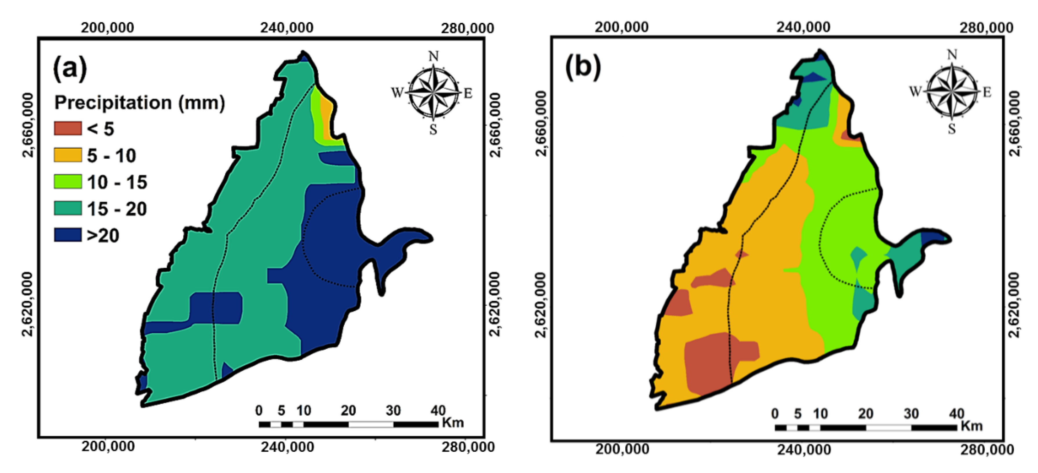
3.1. Modified Precipitation (MoP)
3.2. Linear Regression Analysis
3.2.1. GWL and Land Surface Elevation (DEM)
3.2.2. GWL and MoP
3.2.3. GWL, Land Surface Elevation (DEM), and MoP
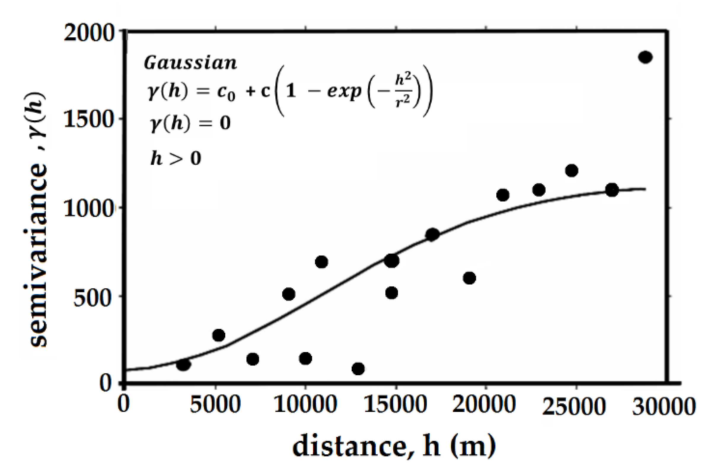
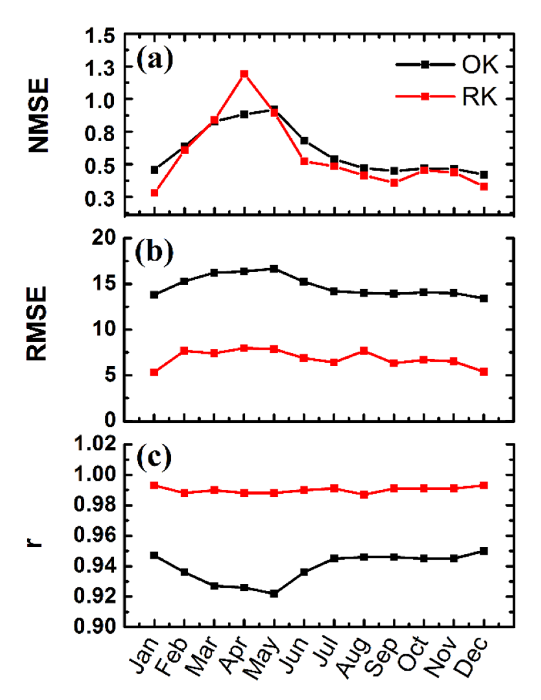
3.3. Geostatistical Interpolation Methods
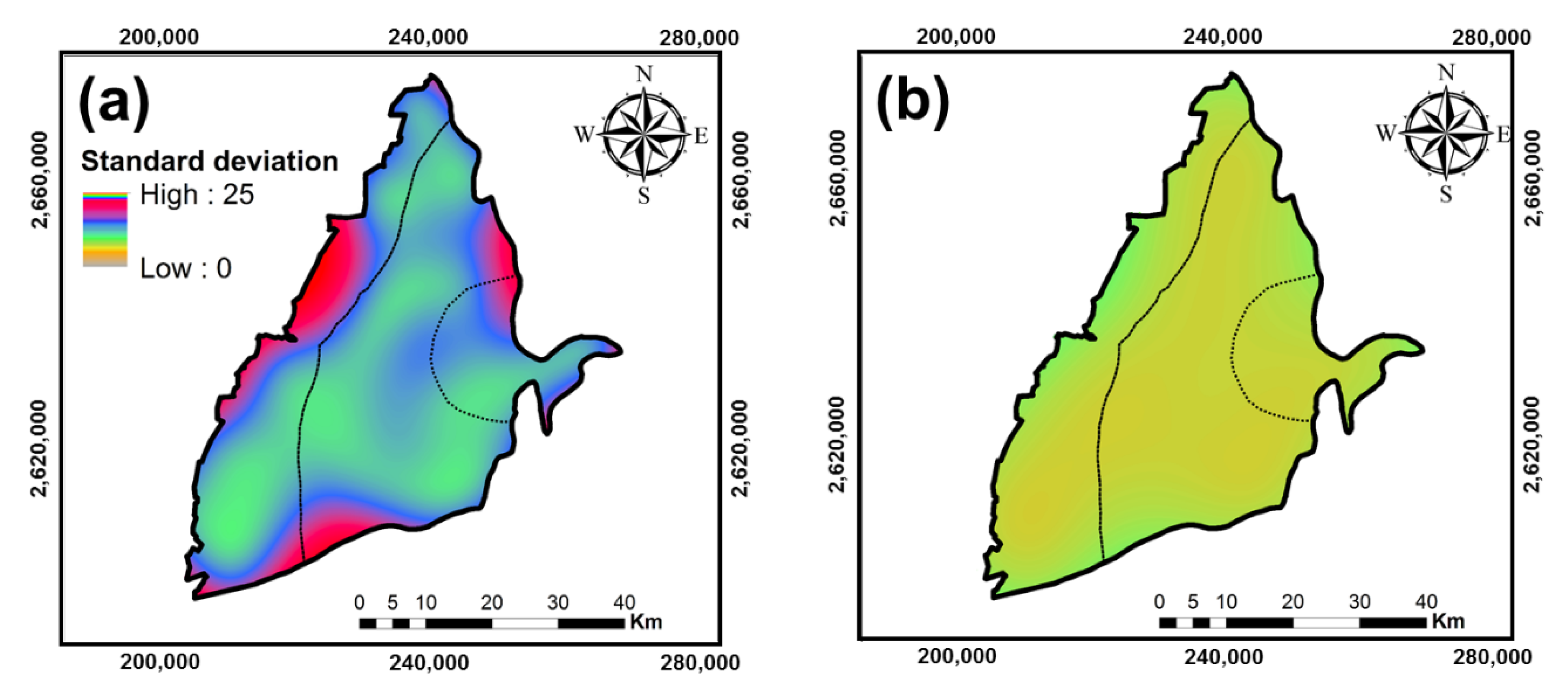
3.4. Assessment Criteria
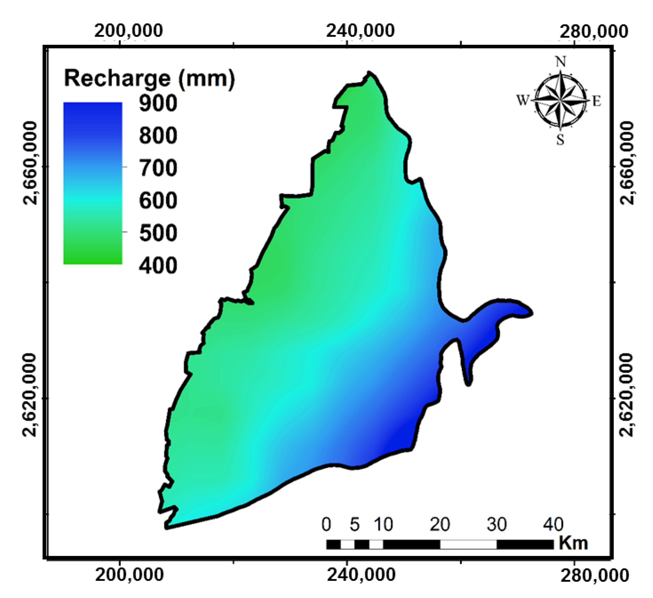
3.5. GWR
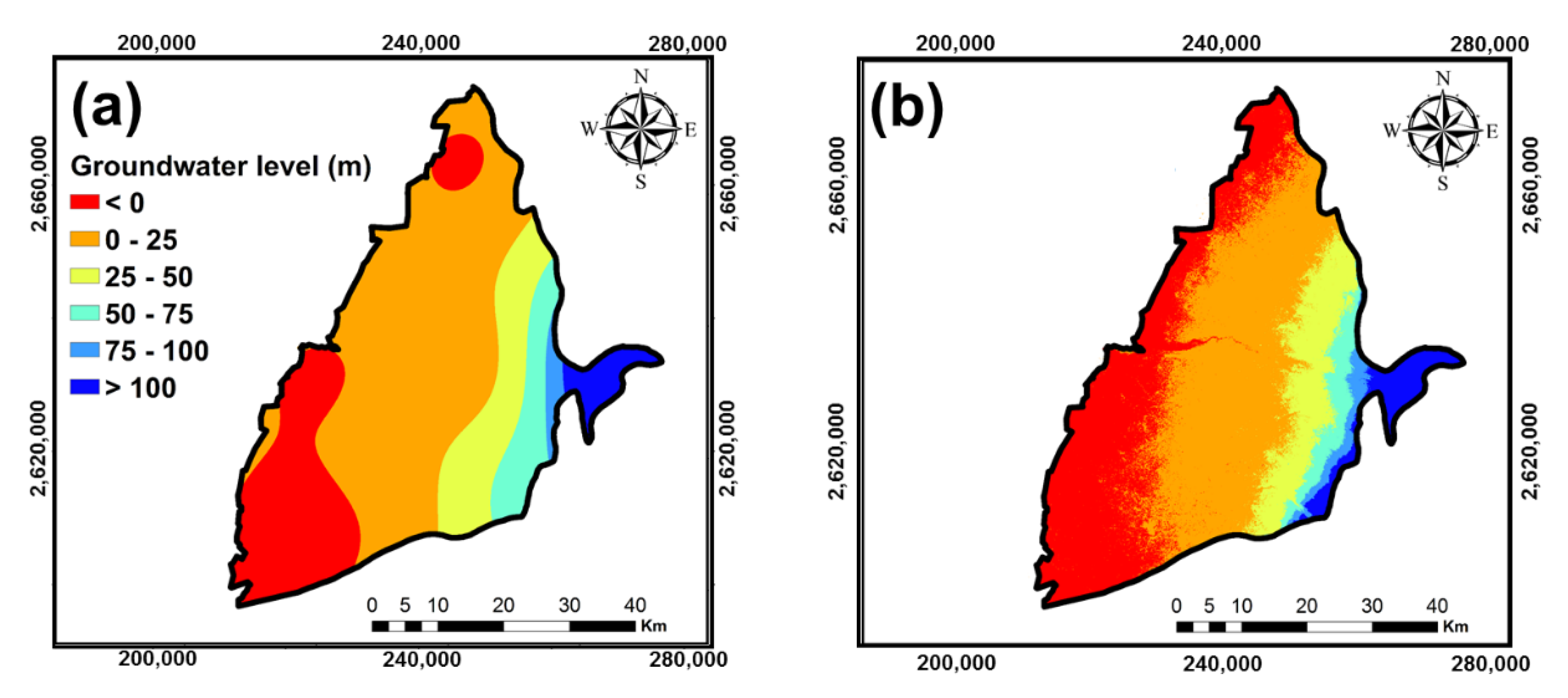
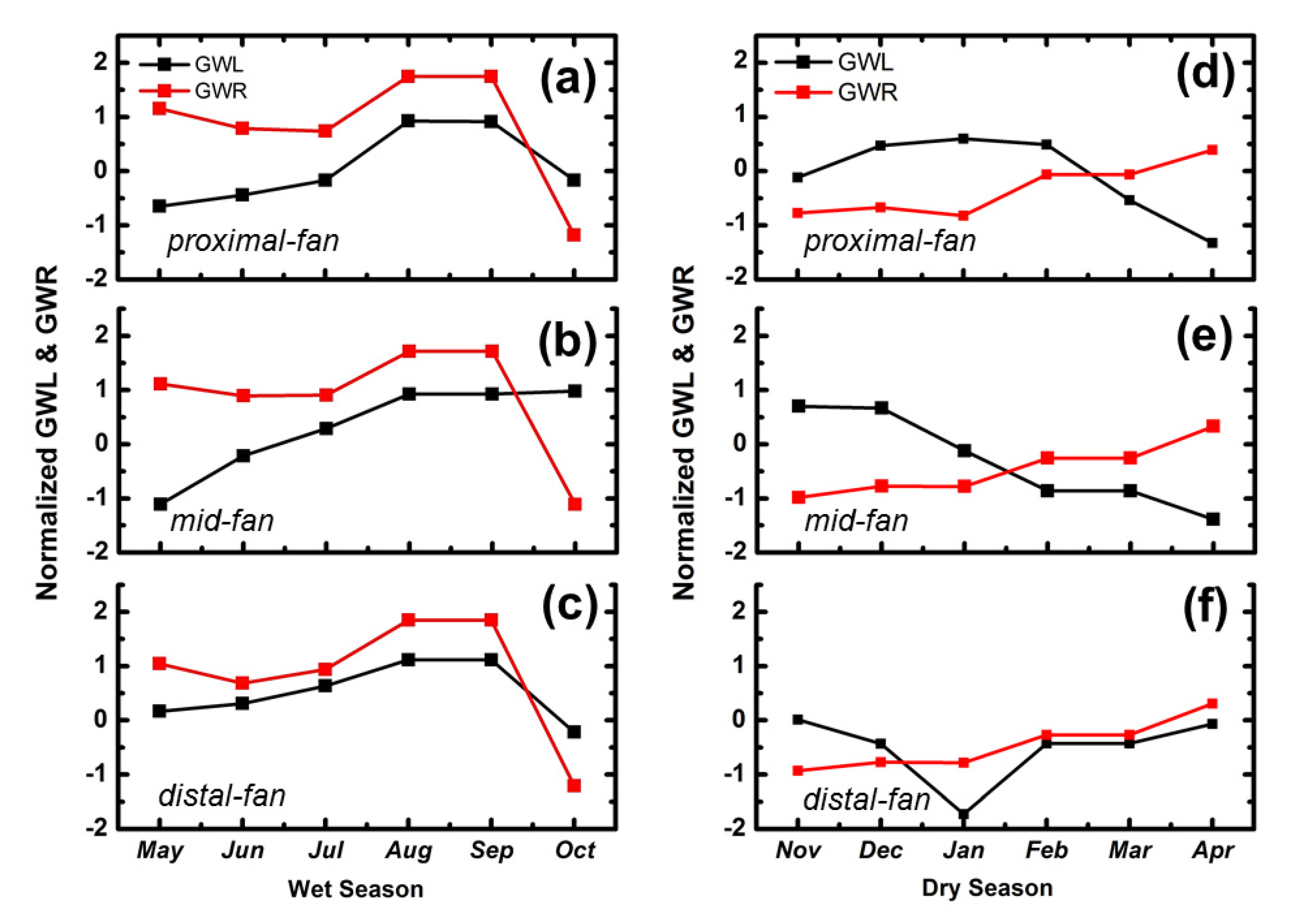
3.6. Spatial-Temporal Variations of GWL and GWR
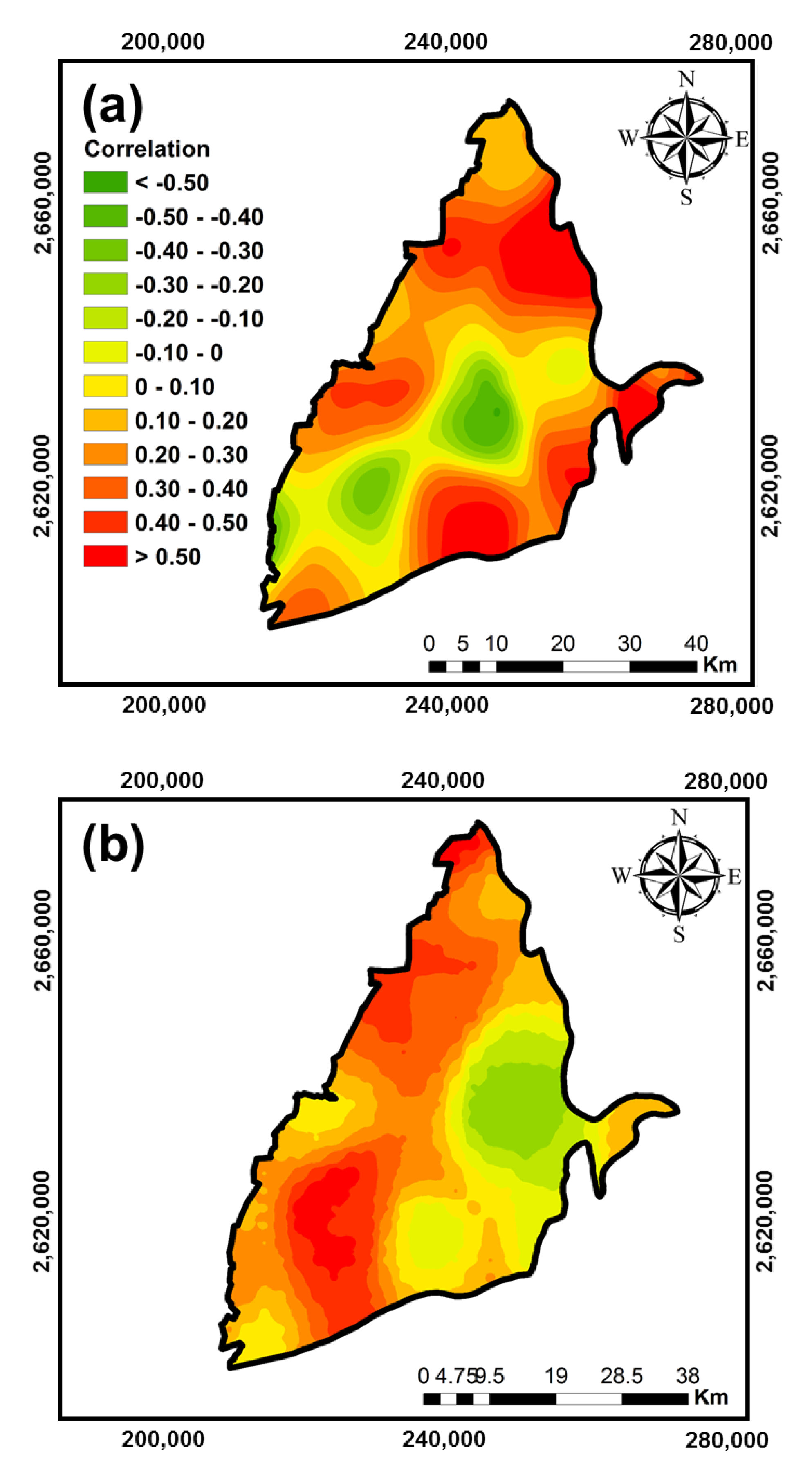
3.7. Event-Based Correlation of GWL and GWR
4. Conclusions
Author Contributions
Funding
Acknowledgments
Conflicts of Interest
References
- Twort, A.C.; Ratnayaka, D.D.; Brandt, M.J. 4-Groundwater Supplies. In Water Supply, 5th ed.; Butterworth-Heinemann: London, UK, 2000; p. 114-II. [Google Scholar]
- Keesstra, S.D.; Geissen, V.; Mosse, K.; Piiranen, S.; Scudiero, E.; Leistra, M.; van Schaik, L. Soil as a filter for groundwater quality. Curr. Opin. Environ. Sustain. 2012, 4, 507–516. [Google Scholar] [CrossRef]
- Keesstra, S.D.; Kondrlova, E.; Czajka, A.; Seeger, M.; Maroulis, J. Assessing riparian zone impacts on water and sediment movement: A new approach. Neth. J. Geosci. Geol. en Mijnb. 2014, 91, 245–255. [Google Scholar] [CrossRef]
- Keesstra, S.D. Impact of natural reforestation on floodplain sedimentation in the Dragonja basin, SW Slovenia. Earth Surf. Process. Landf. 2007, 32, 49–65. [Google Scholar] [CrossRef]
- Keesstra, S.D.; van Dam, O.; Verstraeten, G.; van Huissteden, J. Changing sediment dynamics due to natural reforestation in the Dragonja catchment, SW Slovenia. Catena 2009, 78, 60–71. [Google Scholar] [CrossRef]
- Şen, Z. Chapter 6-Groundwater Management. In Practical and Applied Hydrogeology; Şen, Z., Ed.; Elsevier: Oxford, UK, 2015; pp. 341–397. [Google Scholar]
- Miro, M.; Famiglietti, J. Downscaling GRACE Remote Sensing Datasets to High-Resolution Groundwater Storage Change Maps of California’s Central Valley. Remote Sens. 2018, 10, 143. [Google Scholar] [CrossRef] [Green Version]
- Li, J.; Pei, Y.; Zhao, S.; Xiao, R.; Sang, X.; Zhang, C. A Review of Remote Sensing for Environmental Monitoring in China. Remote Sens. 2020, 12, 1130. [Google Scholar] [CrossRef] [Green Version]
- Lu, C.-H.; Ni, C.-F.; Chang, C.-P.; Chen, Y.-A.; Yen, J.-Y. Geostatistical Data Fusion of Multiple Type Observations to Improve Land Subsidence Monitoring Resolution in the Choushui River Fluvial Plain, Taiwan. Terr. Atmos. Ocean. Sci. 2016, 27, 505. [Google Scholar] [CrossRef] [Green Version]
- Schwenk, J.; Khandelwal, A.; Fratkin, M.; Kumar, V.; Foufoula-Georgiou, E. High spatiotemporal resolution of river planform dynamics from Landsat: The RivMAP toolbox and results from the Ucayali River. Earth Space Sci. 2017, 4, 46–75. [Google Scholar] [CrossRef]
- Lu, C.-H.; Ni, C.-F.; Chang, C.-P.; Yen, J.-Y.; Chuang, R.Y. Coherence Difference Analysis of Sentinel-1 SAR Interferogram to Identify Earthquake-Induced Disasters in Urban Areas. Remote Sens. 2018, 10, 1318. [Google Scholar] [CrossRef] [Green Version]
- Liou, Y.-A.; Mulualem, G.M. Spatio–temporal Assessment of Drought in Ethiopia and the Impact of Recent Intense Droughts. Remote Sens. 2019, 11, 1828. [Google Scholar] [CrossRef] [Green Version]
- Kreklow, J.; Steinhoff-Knopp, B.; Friedrich, K.; Tetzlaff, B. Comparing Rainfall Erosivity Estimation Methods Using Weather Radar Data for the State of Hesse (Germany). Water 2020, 12, 1424. [Google Scholar] [CrossRef]
- Adhikary, S.K.; Muttil, N.; Yilmaz, A.G. Cokriging for enhanced spatial interpolation of rainfall in two Australian catchments. Hydrol. Process. 2017, 31, 2143–2161. [Google Scholar] [CrossRef] [Green Version]
- Li, L.; Huang, G. Groundwater Level Mapping Using Multiple-Point Geostatistics. Water 2016, 8, 400. [Google Scholar] [CrossRef] [Green Version]
- Jeihouni, M.; Delirhasannia, R.; Alavipanah, S.K.; Shahabi, M.; Samadianfard, S. Spatial analysis of groundwater electrical conductivity using ordinary kriging and artificial intelligence methods (Case study: Tabriz plain, Iran). Geofizika 2015, 192–208. [Google Scholar] [CrossRef]
- Hengl, T. A Practical Guide to Geostatistical Mapping, 2nd ed.; University of Amsterdam: Amsterdam, The Netherlands, 2009. [Google Scholar]
- Li, J.; Heap, A.D. Spatial interpolation methods applied in the environmental sciences: A review. Environ. Model. Softw. 2014, 53, 173–189. [Google Scholar] [CrossRef]
- Hengl, T.; Heuvelink, G.B.M.; Rossiter, D.G. About regression-kriging: From equations to case studies. Comput. Geosci. 2007, 33, 1301–1315. [Google Scholar] [CrossRef]
- Kumar, S.; Lal, R.; Liu, D. A geographically weighted regression kriging approach for mapping soil organic carbon stock. Geoderma 2012, 189–190, 627–634. [Google Scholar] [CrossRef]
- Meng, Q.; Liu, Z.; Borders, B.E. Assessment of regression kriging for spatial interpolation—Comparisons of seven GIS interpolation methods. Cartogr. Geogr. Inf. Sci. 2013, 40, 28–39. [Google Scholar] [CrossRef]
- Yao, X.; Fu, B.; Lü, Y.; Sun, F.; Wang, S.; Liu, M. Comparison of Four Spatial Interpolation Methods for Estimating Soil Moisture in a Complex Terrain Catchment. PLoS ONE 2013, 8, e54660. [Google Scholar] [CrossRef]
- Glenn, J.; Tonina, D.; Morehead, M.D.; Fiedler, F.; Benjankar, R. Effect of transect location, transect spacing and interpolation methods on river bathymetry accuracy. Earth Surf. Process. Landf. 2015, 41, 1185–1198. [Google Scholar] [CrossRef]
- Lu, C.H.; Ni, C.F.; Chang, C.P.; Yen, J.Y.; Hung, W.C. Combination with precise leveling and PSInSAR observations to quantify pumping-induced land subsidence in central Taiwan. Proc. IAHS 2015, 372, 77–82. [Google Scholar] [CrossRef] [Green Version]
- Funk, C.; Peterson, P.; Landsfeld, M.; Pedreros, D.; Verdin, J.; Shukla, S.; Husak, G.; Rowland, J.; Harrison, L.; Hoell, A.; et al. The climate hazards infrared precipitation with stations—A new environmental record for monitoring extremes. Sci. Data 2015, 2. [Google Scholar] [CrossRef] [Green Version]
- Goovaerts, P. Applied Geostatistic for Natural Resources Evaluation; Oxford University Press, Inc.: Oxford, UK, 1997. [Google Scholar]
- Burrough, P.A.; Lloyd, C.D. Principles of Geographical Information Systems, 3rd ed.; Oxford University Press: Oxford, UK, 2015. [Google Scholar]
- Bisson, R.A.; Lehr, J.H. Modern Groundwater Exploration: Discovering New Water Resources in Consolidated Rocks Using Innovative Hydrogeological Concepts, Exploration, Drilling, Aquifer Testing and Management Methods; John Wiley & Sons: Hoboken, NJ, USA, 2004; p. 321. [Google Scholar]
- Mishra, S.K.; Singh, V. Soil Conservation Service Curve Number (SCS-CN) Methodology; Water Science and Technology Library; Kluwer Academic Publisher: Dordrecht, The Netherlands, 2003. [Google Scholar]
- Abraham, S.; Huynh, C.; Vu, H. Classification of Soils into Hydrologic Groups Using Machine Learning. Data 2019, 5, 2. [Google Scholar] [CrossRef] [Green Version]
- Anderson, J.R.; Hardy, E.E.; Roach, J.T.; Witmer, R.E. A Land Use and Land Cover Classification System for Use with Remote Sensor Data; Professional Paper 964; The U.S. Geological Survey (USGS) Land Cover Institute (LCI): Sioux Falls, SD, USA, 1976.
- Congalton, R.G.; Green, K. Assessing the Accuracy of Remotely Sensed Data; CRC Press: Boca Raton, FL, USA, 2019; p. 346. [Google Scholar]
- Kumar, V.; Remadevi, V. Kriging of Groundwater Levels—A Case Study. J. Spat. Hydrol. 2006, 6, 81–92. [Google Scholar]
- Mosca, S.; Giovanni, G.; Kluga, W.; Bellasioa, R.; Bianconia, R. A Statistical Methodology for the Evaluation of Long-Range Dispersion Models: An Application to the ETEX Exercise. Atmos. Environ. (ETEX Spec. Issue) 1998, 32, 4307–4324. [Google Scholar] [CrossRef]
- Feidas, H.; Kokolatos, G.; Negri, A.; Manyin, M.; Chrysoulakis, N.; Kamarianakis, Y. Validation of an infrared-based satellite algorithm to estimate accumulated rainfall over the Mediterranean basin. Theor. Appl. Climatol. 2008, 95, 91–109. [Google Scholar] [CrossRef]
- Li, J.; Heap, A.D. A review of comparative studies of spatial interpolation methods in environmental sciences: Performance and impact factors. Ecol. Inform. 2011, 6, 228–241. [Google Scholar] [CrossRef]
- Şen, Z. Chapter Six-Climate Change, Droughts, and Water Resources. In Applied Drought Modeling, Prediction, and Mitigation; Şen, Z., Ed.; Elsevier: Boston, MA, USA, 2015; pp. 321–391. [Google Scholar]
- Lin, H.-T.; Ke, K.-Y.; Tan, Y.-C.; Wu, S.-C.; Hsu, G.; Chen, P.-C.; Fang, S.-T. Estimating Pumping Rates and Identifying Potential Recharge Zones for Groundwater Management in Multi-Aquifers System. Water Resour. Manag. 2013, 27, 3293–3306. [Google Scholar] [CrossRef]
- Tsai, J.-P.; Chen, Y.-W.; Chang, L.-C.; Kuo, Y.-M.; Tu, Y.-H.; Pan, C.-C. High Recharge Areas in the Choushui River Alluvial Fan (Taiwan) Assessed from Recharge Potential Analysis and Average Storage Variation Indexes. Entropy 2015, 17, 1558–1580. [Google Scholar] [CrossRef] [Green Version]
- Sorí, R.; Nieto, R.; Vicente-Serrano, S.M.; Drumond, A.; Gimeno, L. A Lagrangian perspective of the hydrological cycle in the Congo River basin. Earth Syst. Dyn. 2017, 8, 653–675. [Google Scholar] [CrossRef] [Green Version]


| Main Variable | Secondary Variables | r | r2 | p-Value | Significance |
|---|---|---|---|---|---|
| GWL | Surface Elevation (DEM) | 0.97 | 0.95 | 2.2 × 10⁻⁶ | DEM (significant) |
| GWL | MoP | 0.70 | 0.49 | 5.4 × 10⁻⁶ | MoP (significant) |
| GWL | Surface Elevation, MoP | 0.97 | 0.95 | 2.2 × 10⁻⁶ | DEM (significant) MoP (insignificant) |
| DEM | MoP | 0.68 | 0.46 | 1.55 × 10⁻⁵ | MoP (significant) |
| Land ID | Land Use | Area (km2) | CN for HSG | CN × Area | |||
|---|---|---|---|---|---|---|---|
| A | B | C | D | Total Area (km2) | |||
| 1 | Water | 60.25 | 98 | 98 | 98 | 98 | 5904.75 |
| 2 | Mix Forest | 66.90 | 35 | 60 | 73 | 80 | 2341.43 |
| 3 | Grassland | 133.98 | 49 | 70 | 80 | 85 | 6564.82 |
| 4 | Wetlands | 43.69 | 25 | 55 | 70 | 77 | 1092.25 |
| 5 | Crop lands | 1159.52 | 44 | 66 | 77 | 83 | 51,018.88 |
| 6 | Urban area | 255.84 | 54 | 70 | 80 | 85 | 13,815.09 |
| 7 | Bare soils | 569.17 | 35 | 61 | 74 | 80 | 19,920.81 |
| Total | 2289.34 | 100,658.03 | |||||
| Composite Curve Number (CCN) | 44 | ||||||
Publisher’s Note: MDPI stays neutral with regard to jurisdictional claims in published maps and institutional affiliations. |
© 2020 by the authors. Licensee MDPI, Basel, Switzerland. This article is an open access article distributed under the terms and conditions of the Creative Commons Attribution (CC BY) license (http://creativecommons.org/licenses/by/4.0/).
Share and Cite
Nainggolan, L.; Ni, C.-F.; Darmawan, Y.; Lee, I.-H.; Lin, C.-P.; Li, W.-C. Data-Driven Approach to Assess Spatial-Temporal Interactions of Groundwater and Precipitation in Choushui River Groundwater Basin, Taiwan. Water 2020, 12, 3097. https://doi.org/10.3390/w12113097
Nainggolan L, Ni C-F, Darmawan Y, Lee I-H, Lin C-P, Li W-C. Data-Driven Approach to Assess Spatial-Temporal Interactions of Groundwater and Precipitation in Choushui River Groundwater Basin, Taiwan. Water. 2020; 12(11):3097. https://doi.org/10.3390/w12113097
Chicago/Turabian StyleNainggolan, Lamtupa, Chuen-Fa Ni, Yahya Darmawan, I-Hsien Lee, Chi-Ping Lin, and Wei-Ci Li. 2020. "Data-Driven Approach to Assess Spatial-Temporal Interactions of Groundwater and Precipitation in Choushui River Groundwater Basin, Taiwan" Water 12, no. 11: 3097. https://doi.org/10.3390/w12113097