The Effect of Small Density Differences at River Confluences


1
Faculty of Civil Engineering and Geosciences, Delft University of Technology, 2628CN Delft, The Netherlands
2
Deltares, 2629HV Delft, The Netherlands
*
Author to whom correspondence should be addressed.
†
Current address: Laboratory of Hydraulics, Hydrology and Glaciology, ETH Zürich.
Water 2020, 12(11), 3084; https://doi.org/10.3390/w12113084
Submission received: 12 October 2020
/
Revised: 28 October 2020
/
Accepted: 30 October 2020
/
Published: 3 November 2020
(This article belongs to the Section Hydraulics and Hydrodynamics)
Abstract
:Remarkable 3D flow structures occur at river confluences with small density differences due to differences in sediment concentration or temperature. We explain these by comparing numerical simulations for an idealized confluence with aerial photographs of several river confluences where color differences express the pattern of density differences at the surface. We analyzed numerical simulations of the Rio Negro–Solimões confluence near Manaus, Brazil, in more detail. The numerical model of the idealized confluence showed that the dense water flowed under the light water and the light water over the dense water in a spiraling motion, distorting the interface between the two waters. The horizontal part of this interface moves upwards in downstream direction. Constraining of the spiraling motion in a narrow river downstream of the confluence can cause local up- and downwelling near the banks. A mixing layer can develop when the flow velocities of the two tributaries differ, but strong spiraling motion due to the density differences can suppress this development. The aerial photographs and all numerical simulations showed similar density patterns at the water surface. Even small density differences can have a significant impact and hence need to be considered when analyzing and modeling 3D flow at confluences.
1. Introduction
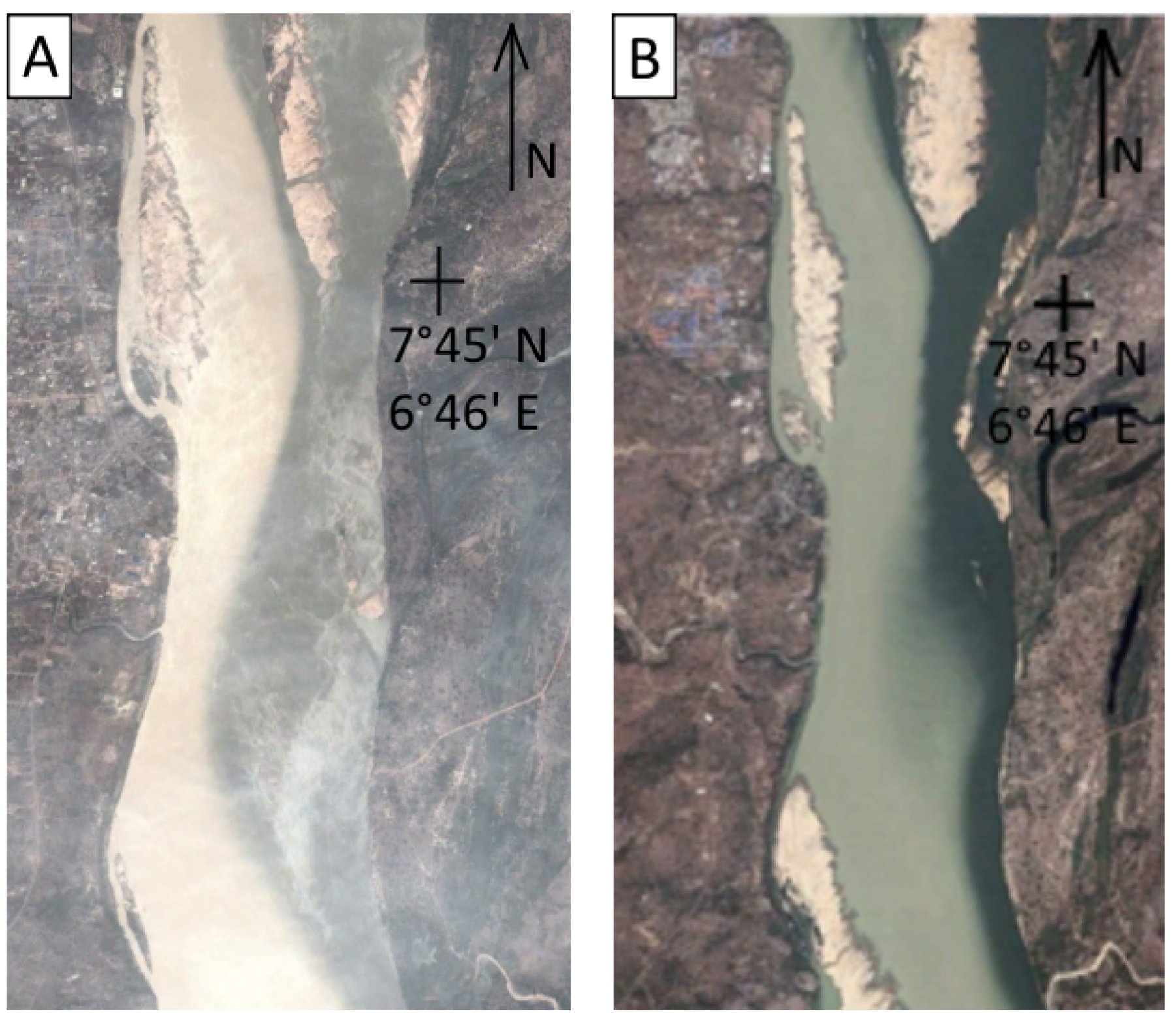
The merging of rivers at confluences gives rise to intriguing phenomena at the water surface, which are visible on aerial photographs (Figure 1). In these photographs, one tributary has a lighter color than the other, thus revealing where water from each tributary goes. The Benue water in Figure 1A initially occupies an increasingly larger part of the surface width. However, below a certain location it is the Niger water that occupies an increasingly larger proportion of the surface width. This increase of dark-colored water at the surface is also visible in Figure 1B. Additionally, Figure 1B shows a mixing layer which is absent in Figure 1A. These phenomena are relevant for the routing of pollutants or sediment and the assessment of ecological impacts [1,2].
Best [3] discusses the general flow dynamics at confluences. He defines six elements downstream of a confluence: stagnation zone, flow deflection zone, flow separation zone, maximum velocity zone, flow recovery zone, and shear layers. For nonzero confluence angles, the flow deflection zone and shear layer are impacted by the momentum ratio, M, of the two tributaries [4]: , where u is the velocity, Q the discharge, the water density, and the subscripts 1 and 2 refer to the two tributaries.
On a large scale, the amount of mixing downstream of a confluence may depend on the locations where side channels diverge and merge again with the main channel [5]. On a more local scale, different types of complex flows can alter the flow dynamics and cause small deviations at the water surface [6]. If, for instance, the two tributaries meet under a nonzero angle, the realignment of the tributaries to the downstream channel direction implies curved flow, which generates helical flow cells like those in a meander [7,8,9]. In a symmetrical confluence, two helical cells will form [10], but only one cell if one of the tributaries has much more momentum than the other one, expressed by the momentum ratio [7]. Curved incoming channels produce helical flow, as well. For nonzero confluence angles, the location of the shear layer depends on the momentum ratio. It will be located approximately in the center of the channel downstream if the momentum ratio is close to 1 [4]. If the confluence angle equals zero, the shear layer moves towards the side with the lower velocity [11,12]. Due to differences in bed level (bed discordance), the water of one of the tributaries may flow under the water of the other tributary [13,14]. In some cases, this can lead to upwelling of water from one tributary near the bank of the other tributary [15].
When two tributaries have different velocities, a mixing layer may develop around the shear layer. Here, coherent structures can develop that enhance the lateral mixing [16], although they may not always be efficient in mixing [17]. They can be similar to coherent structures forming in the wake of an obstruction or to those in a classical mixing layer [18,19,20]. This likely depends on where the boundary layer detaches, and hence on discharge and local bathymetry. Bed discordance may distort the coherent structures in the mixing layer [21].
For coherent structures to develop, the flow needs to be unstable. Daoyi and Jirka [22] show that coherent structures develop only if the stability number is smaller than 0.1. Here, is a dimensionless friction parameter, l a length scale, the mean velocity, h the depth, and the velocity difference. An appropriate length scale is the width of the mixing layer. If the width of the mixing layer becomes equal to or larger than the water depth, the mixing layer becomes predominantly two-dimensional.
The features in Figure 1 cannot be adequately explained by bed discordance, flow realignment, curvature-induced flow or momentum ratio differences. Proper explanation seems to require another process. The color difference between the tributaries suggests that the tributaries have different concentrations of suspended sediment. As this may lead to differences in fluid density, we hypothesize that density differences may explain the observed features.
Studies on density differences usually focus on salt intrusion in estuaries (e.g., Reference [23]), on the lock exchange problem (e.g., Reference [24]), or on the mathematical background of stratified flows (e.g., Reference [25]). Little research has been carried out on the effect of density differences at confluences. Rare examples are the work by Cook and Richmond [26], Lyubimova et al. [27], and Ramón et al. [28]. They show that density differences between rivers due to sediment load or temperature tend to be smaller than density differences due to salinity between different zones in estuaries. They qualitatively describe the effects of density differences on the flow patterns at a specific confluence but do not analyze the corresponding physical processes. We aim to fill this gap. Understanding the physical processes due to density differences is especially important since the amount of mixing at confluences is often measured by measuring how the temperature difference changes downstream [9,17,29], even though the temperature affects the density.
We use a physics-based numerical model to investigate which effects of density differences occur in an idealized confluence. The results of the model were compared with aerial photographs of several confluences on which color differences express the pattern of density differences at the surface. The confluence of the Rio Negro and Solimões, near Manaus, Brazil, was analyzed in more detail and compared to both aerial photographs and the results from the idealized model. We specifically considered the large-scale flow structure and the development of the mixing layer.
2. Methods
In order to analyze the effects of density differences in isolation, other phenomena that might play a role at confluences must be excluded. Using an idealized model set-up allows for this. We choose to run numerical models as these have the advantage that the effects of individual parameters can be investigated systematically. We used the Delft3D software (version: 3.15.34158), a physics-based numerical shallow-water-equations solver [30], to make a hydrodynamic model of an idealized confluence in which the effects of bed discordance and confluence angle are absent.
The computational domain of the baseline model was 30 km long and 4830 m wide. The two tributaries were initially separated by a 600-m-long row of dry points and were each half as wide as the downstream river. The bed was horizontal. We used 20 -layers which provided enough vertical spatial resolution. The k- turbulence model was used for all simulations. This is a common turbulence model and is the turbulence model with the highest order that is available in Delft3D.
Inflow discharges were set at the two upstream boundaries and a water level was prescribed at the downstream boundary. The HLES module for horizontal large-eddy simulation was used with a 40-min relaxation time to reproduce coherent structures in the mixing layer. Small disturbances were added at the inflow boundaries to create instabilities that could grow into the coherent turbulent structures. The local specific discharges at the inflow boundaries were randomly drawn at each time step from a Gaussian distribution with a standard deviation of 2% of the mean value. The model was run long enough to reach average stationary conditions, after which the last 10 min of the simulation were analyzed.
Density differences were modeled by giving the tributaries different temperatures. This ensured that the density difference was constant over the vertical, which would not be the case when modeling density differences by giving the tributaries different suspended sediment loads. The baseline temperature difference of 2 C corresponded to a density difference of approximately 0.5 kg/m3, which is significantly smaller than density differences between fresh and saline water in estuaries.
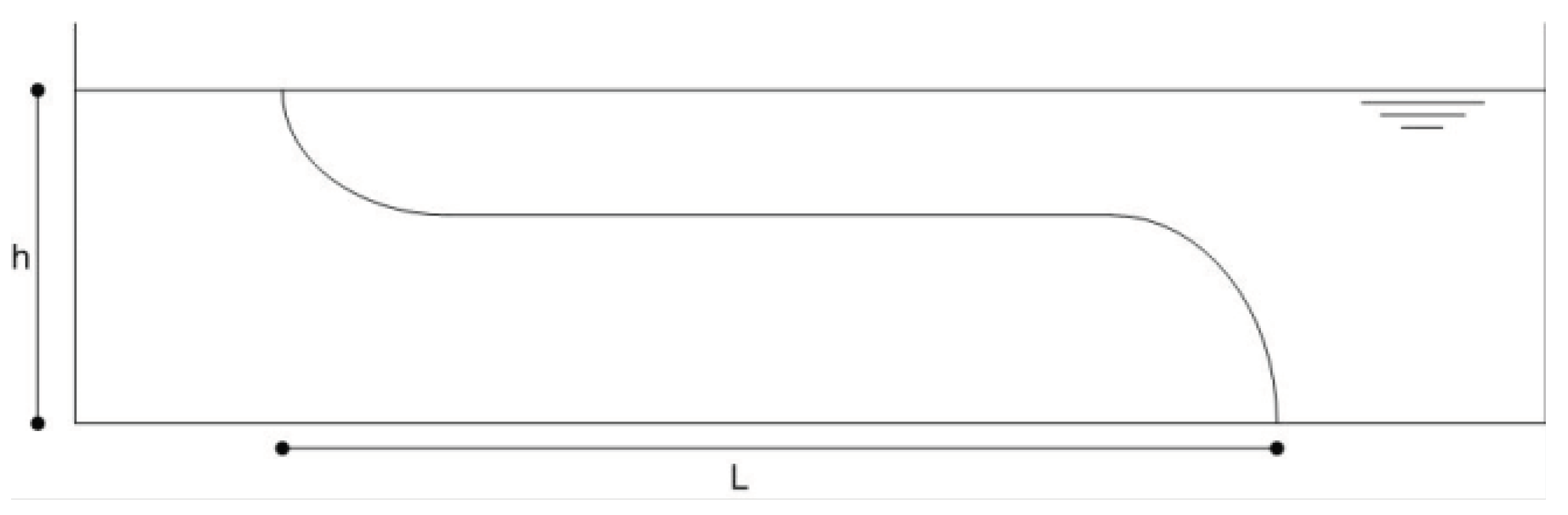
The model was run for a base scenario and for different alternative settings of the model parameters (Table 1). For each of these model runs, the length over which the two waters had flown over one another (L) was computed at 2 km and at 4.5 km downstream of the confluence apex. This length is defined in a cross-section as the horizontal length between the points at the surface and bottom where the average density was present (Figure 2).
We also investigated scenarios of changing both depth and velocity ratio or both density difference and velocity ratio (Table 1). In case the width or depth was varied, the upstream discharge boundary condition was changed in such a way that the velocity remained the same.
In the model runs with a velocity difference, sometimes coherent structures developed around the interface between light and dense water. Coherent structures can be expected to move the point of mean density in a cross-section from left to right. If we found this point to have shifted more than 5 grid cells, we concluded that coherent structures were present. We analyzed this for the top layer and the layer above the bottom layer, in the last 10 min of each simulation.
For all model runs we computed the non-dimensional velocity difference and the Richardson number, , at the confluence apex. Here, Fd is the densimetric Froude number, g is the gravitational acceleration, the height of the density current, the density difference, the mean density, and the mean velocity. The non-dimensional velocity difference is often linked to the occurrence of coherent structures [16,31], whereas the Richardson number characterizes the hydrodyamic effects of density differences. We related the occurrence and non-occurrence of the coherent structures to these two non-dimensional parameters.
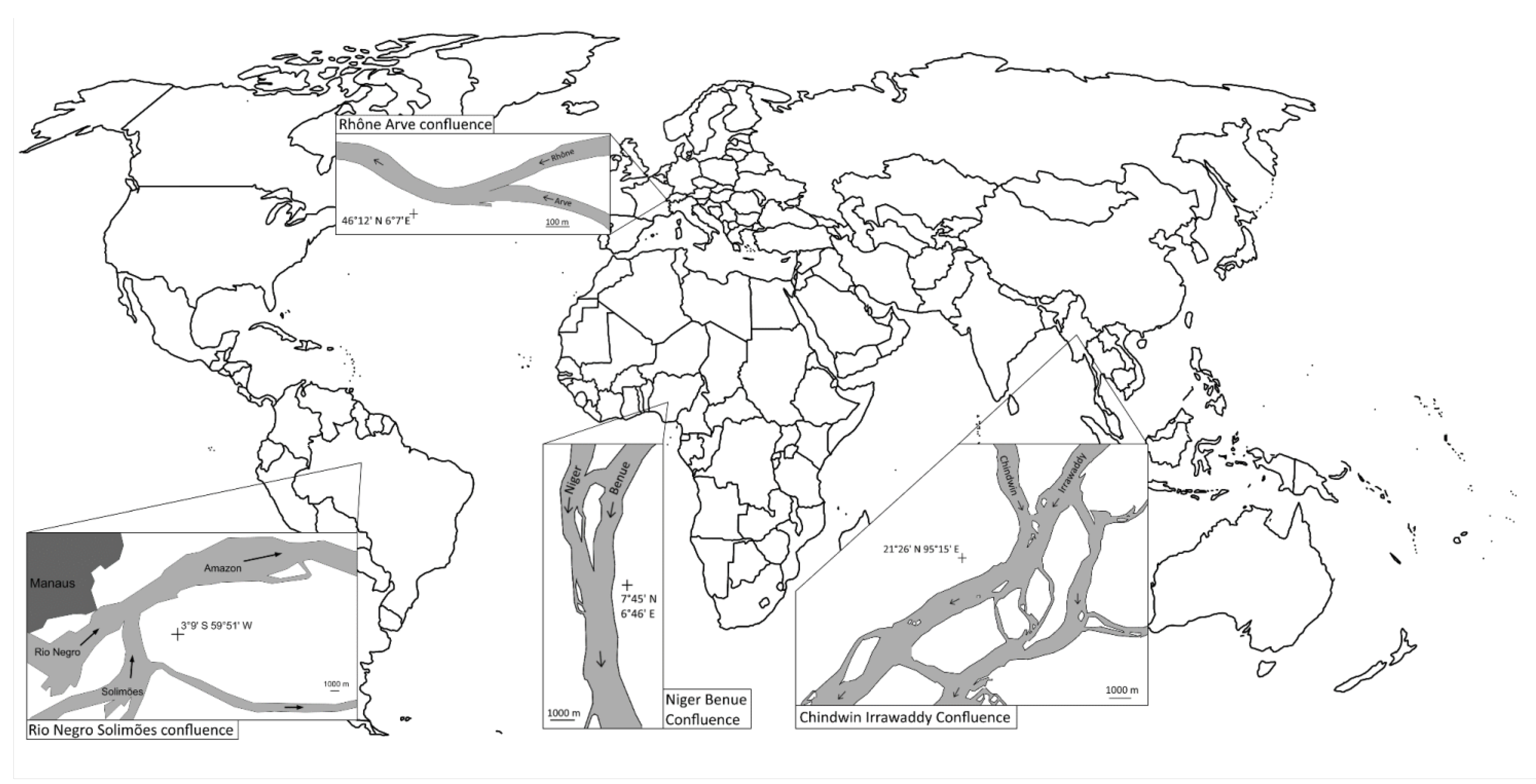
At confluences, the two tributaries can have different colors when sediment concentrations are different. A color difference thus often indicates a density difference. Therefore, aerial photographs can give snapshots of the hydrodynamics at confluences of tributaries with different densities. We analyzed the patterns of several confluences around the globe using Google Earth, focusing on larger rivers where image resolution does not impede pattern recognition. We selected photographs that showed a clear color difference between the tributaries and did not exhibit pronounced bends. This resulted in three suitable confluences for analysis: the Niger–Benue confluence in Nigeria, the Chindwin–Irrawaddy confluence in Myanmar and the Rhône–Arve confluence in Switzerland (Figure 1, Figure 2, Figure 3, Figure 4 and Figure 5). The patterns visible at the water surface on the selected aerial photographs were compared to those found in the numerical model runs.
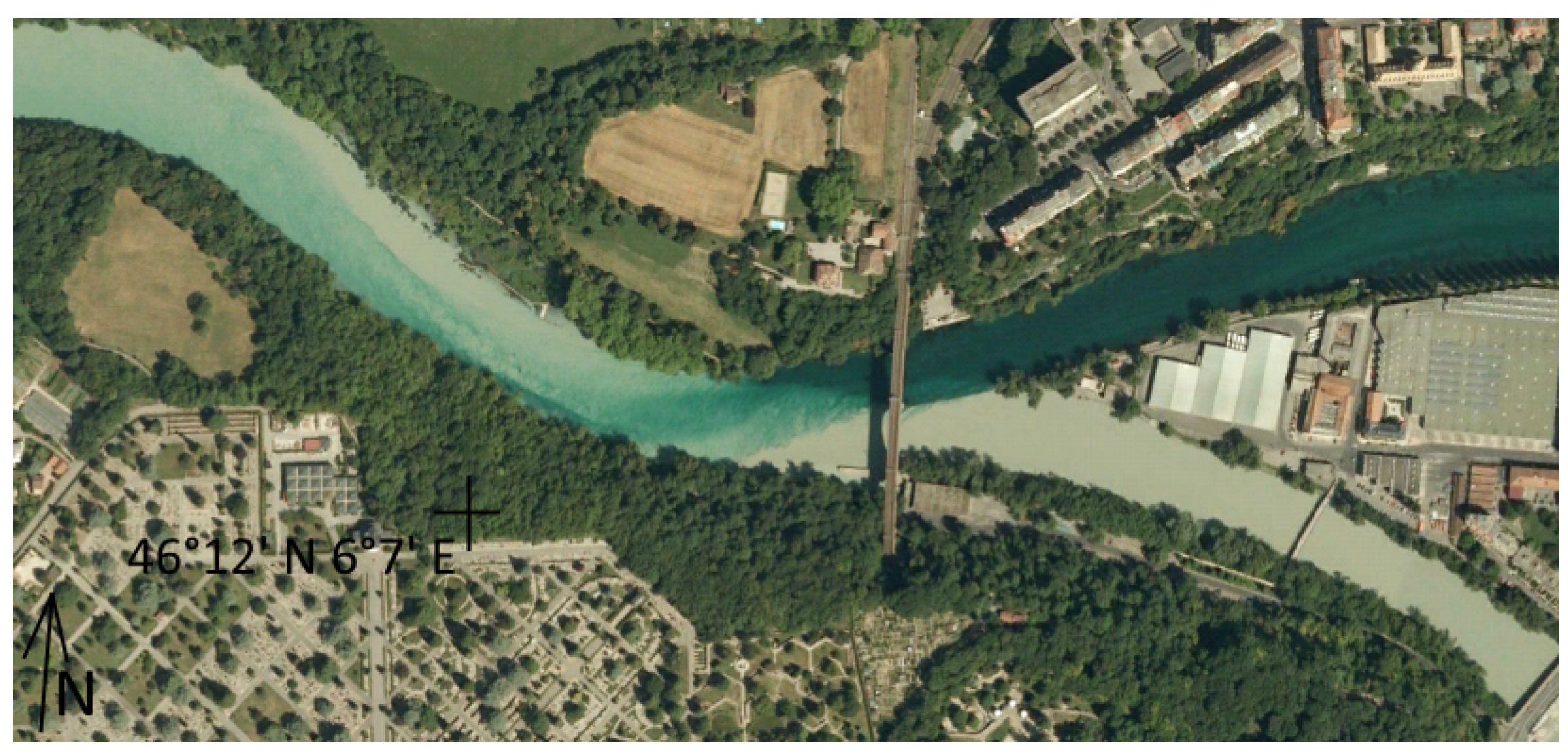
In the Niger–Benue confluence the confluence angle is rather small and there are no bends in the reach. For this confluence, two images, taken at different times, were found with a distinct color difference (Figure 1). The Chindwin–Irrawaddy confluence also has a small confluence angle (Figure 3). Downstream the channel bends to the true right. The confluence of the Rhône and Arve is the smallest of those found (Figure 4). Up to the bridge the waters of these two rivers are separated by a low wall, not overtopped at the time of taking the photograph. The confluence angle was thus 0.
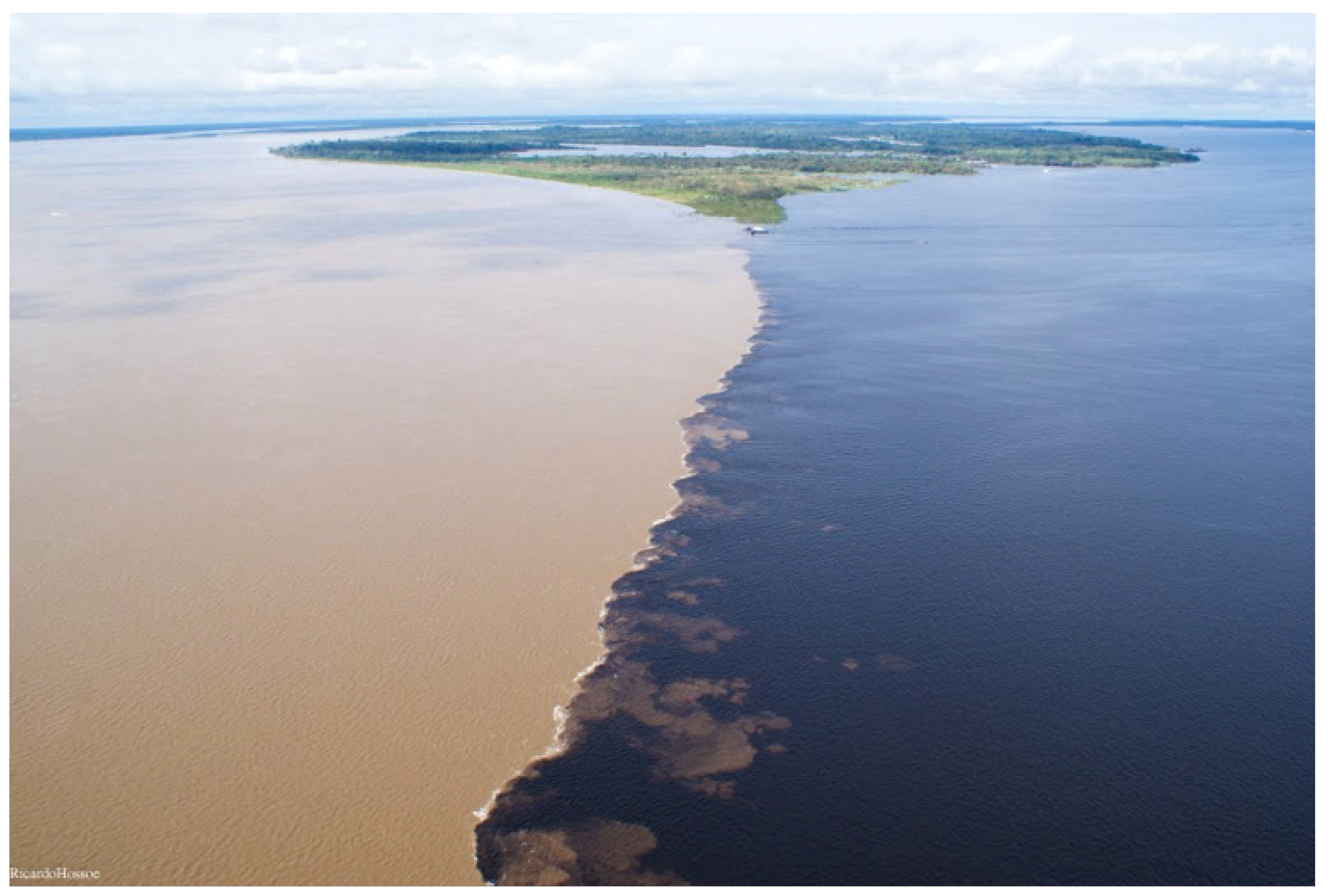
A similar flow pattern can be found at a popular tourist attraction: the merging of the Rio Negro and Solimões near Manaus, Brazil (Figure 5). The two merging tributaries have different colors. For this confluence, we made a separate hydrodynamic model (using Delft3D), comparing its results to both orthogonal and oblique aerial photographs. We carried out three model runs: one for a high water, one for low water, and one for a high momentum ratio between the tributaries (Table 2). Values of discharges, temperatures, and sediment concentrations were based on ANA (2016) [32], Laraque et al. [33], Trevethan et al. [34], and Richey et al. [35]. The resulting density differences were between 0.27 and 0.38 kg/m3. This is comparable to the density differences measured in this confluence (cf. Reference [36]).
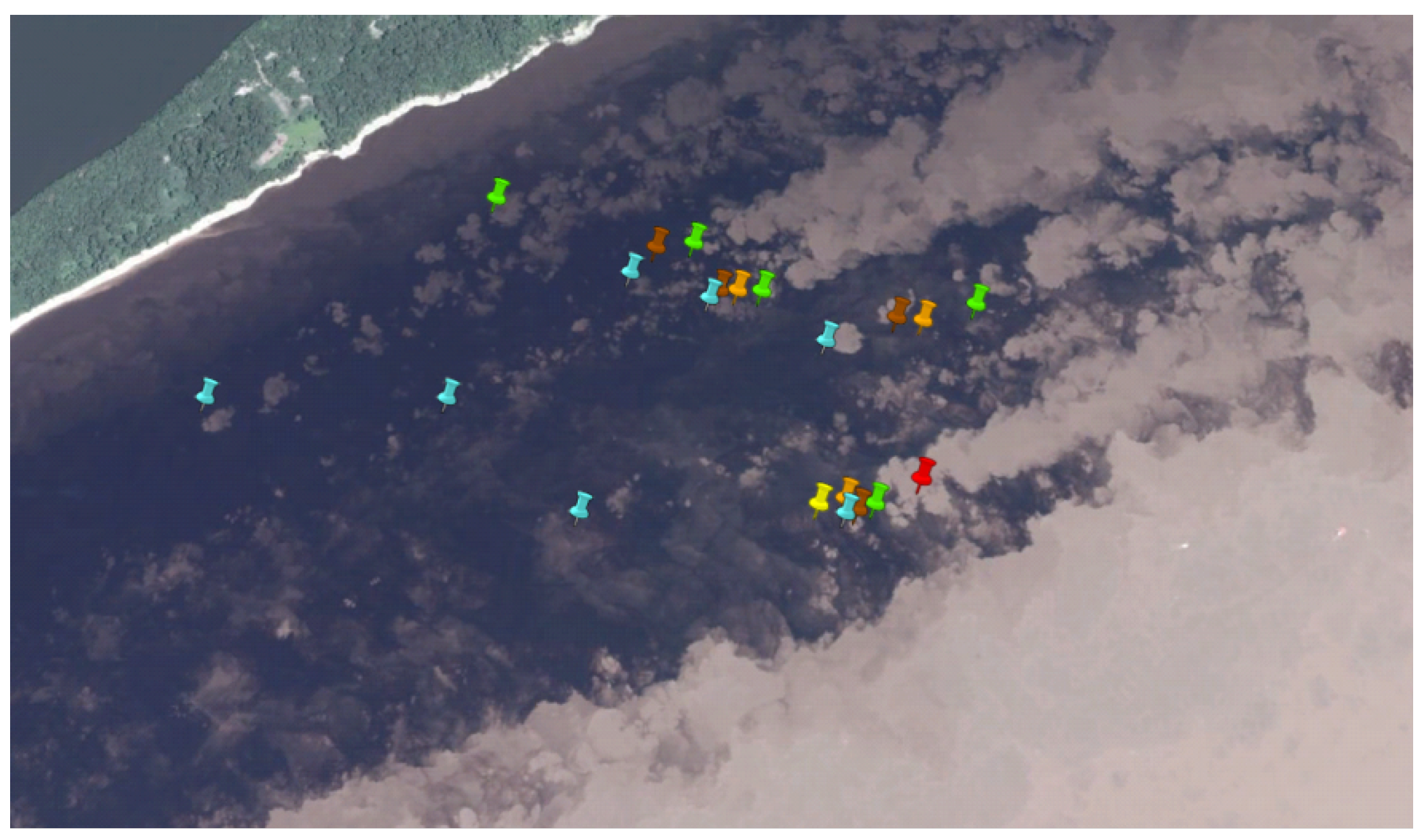
The waters of the Rio Negro and Solimões barely mix. However, specks of light-colored Solimões water were seen on the Rio Negro side of the river. These specks formed lines. Markers were placed at the most upstream speck of each of these lines on all aerial photographs showing the specks, to allow tracking of locations where these specks originated from.
3. Results
3.1. Large-Scale Patterns
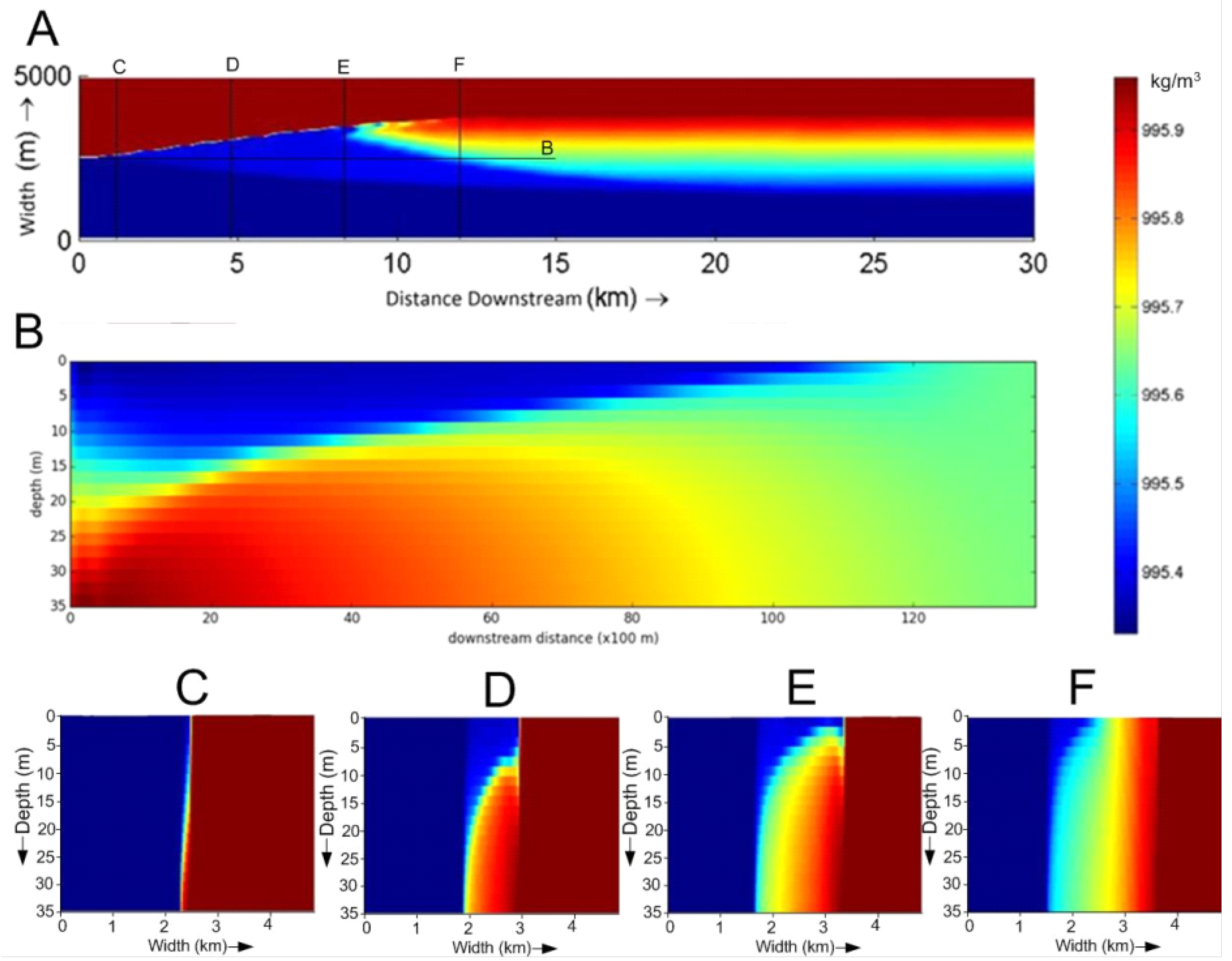
In all numerical runs, large scale patterns of water movement were observed, where the dense water flowed under the lighter water and the lighter water over the dense water (Figure 6 and Figure 7A). As a result, the shear layer between the two waters tilted and became approximately horizontal in its center. This horizontal interface moved upwards when moving in downstream direction and eventually reached the surface, at which point the water around the interface had mixed (Figure 6 and Figure 7A).
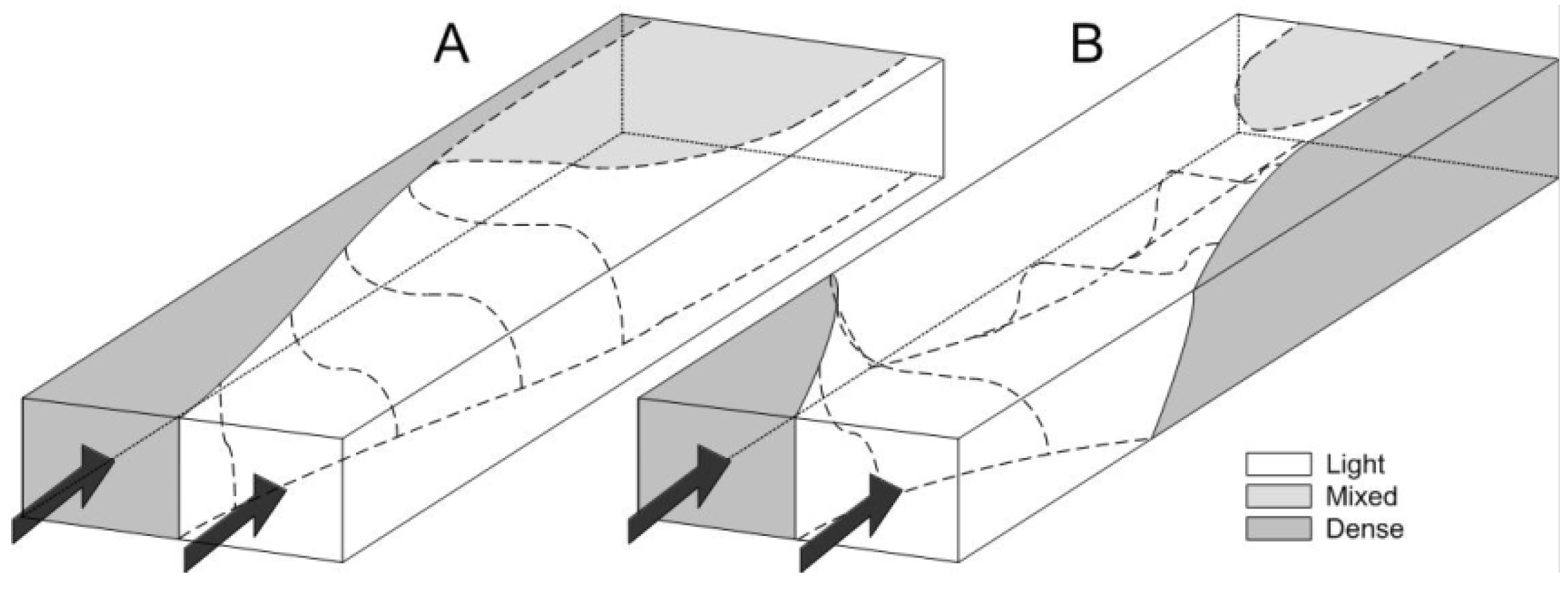
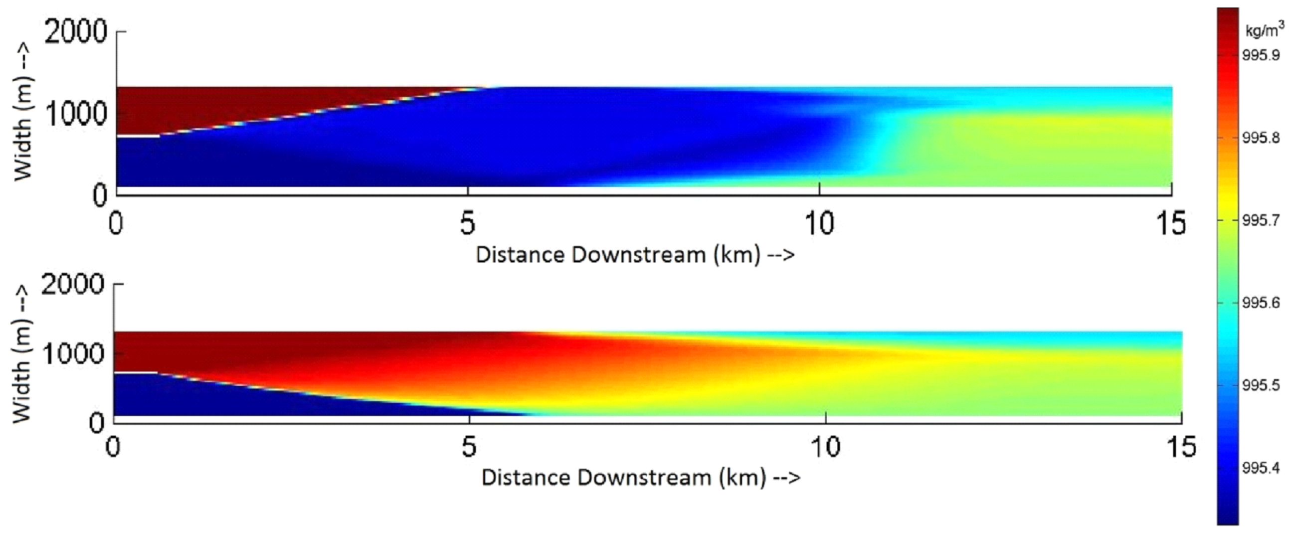
This flow pattern was altered if the downstream section of the river was narrow (Figure 8). With narrow, we here mean that the two waters flowing over one another reached the opposite banks before the horizontal part of the interface between these two waters reached the surface. If this occurs, the dense water will flow vertically upwards along the bank and the light water will flow vertically downwards along the bank (Figure 7B and Figure 8). The vertical flow along the banks is similar to what may occur when the waters reach the banks when the bed is discordant [15]. The location where the horizontal interface between the dense and light water reaches the surface depends on the velocity difference between the tributaries and the roughness.
The large-scale flow patterns can be summarized as follows: The flow of dense water under light water and light water over dense water produces a helical flow. The corresponding circulation cell grows in downstream direction until the horizontal interface reaches the surface if the river downstream is wide. The size of the helical flow cell is restricted if the river downstream is narrow.
3.2. Effect on the Mixing Layer
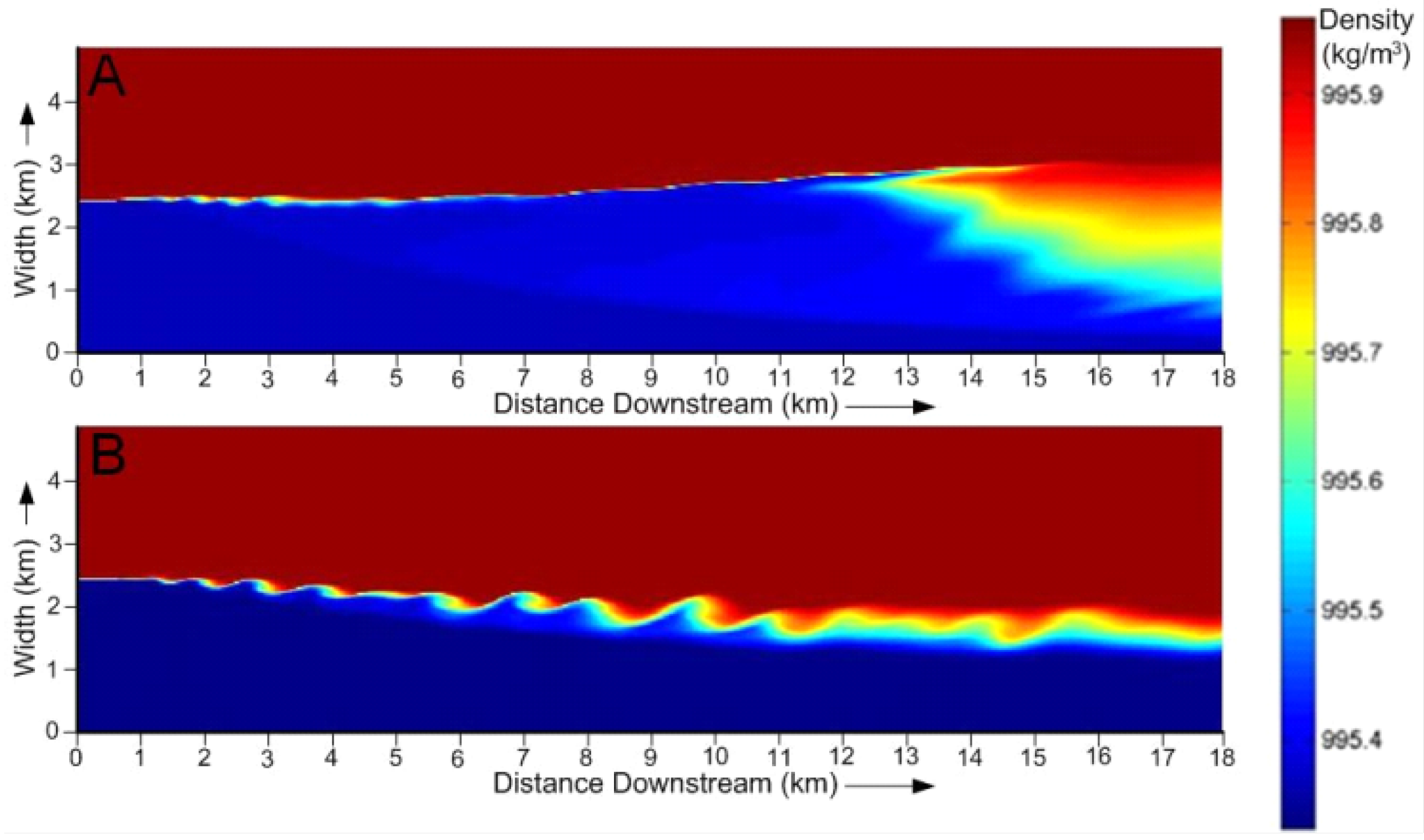
The circulation of the water affects the processes in the mixing layer. Figure 9 shows two cases with equal velocity differences but different density differences and, hence, different water motions perpendicular to the main flow. Besides, the expected differences in the position of the interface at the surface, also pronounced differences arose in the coherent structures. Coherent structures formed at small density differences, not at large density differences.
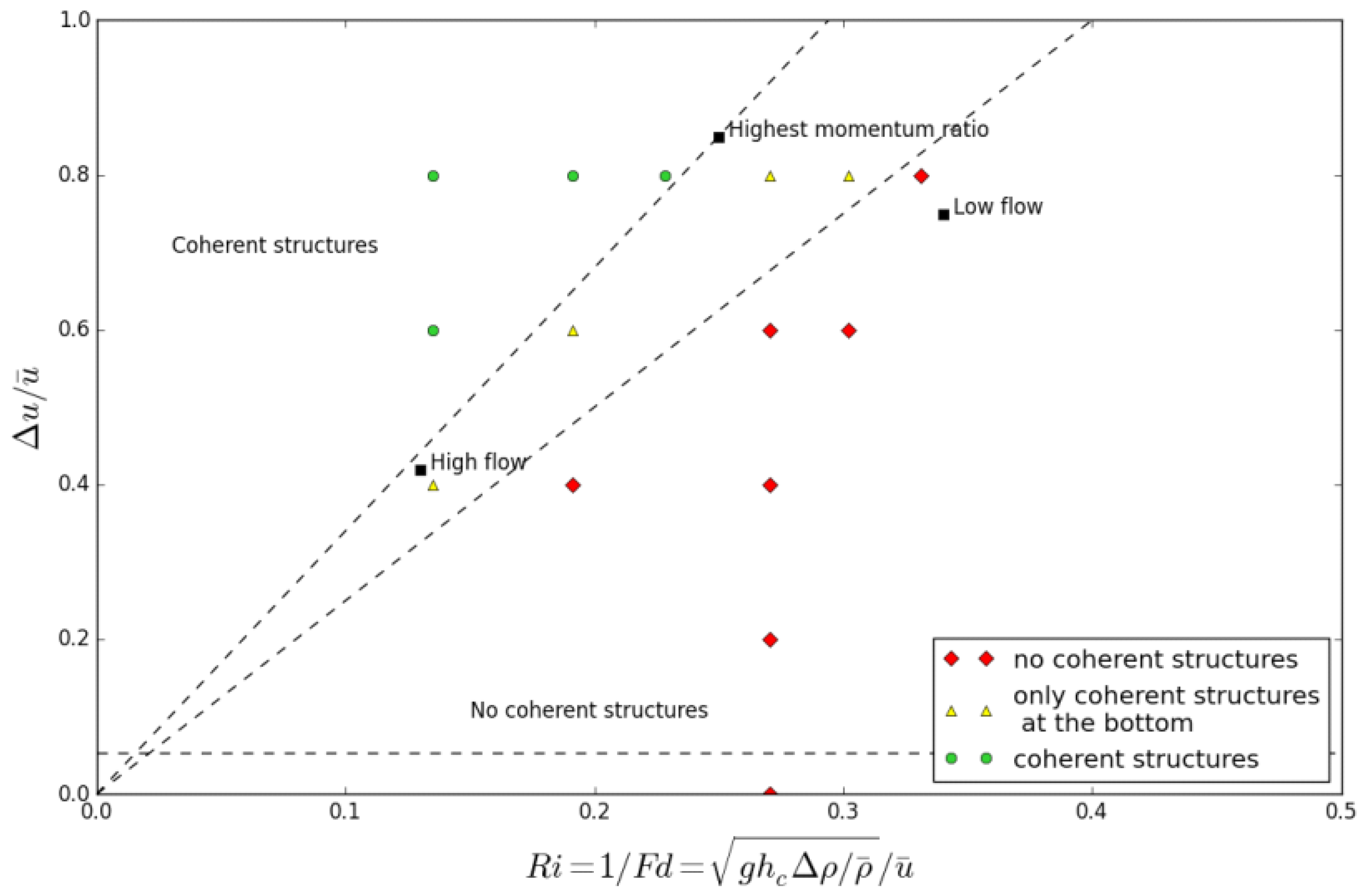
After categorizing every model run with a velocity difference as having or not having coherent structures (Figure 10), we found that the Richardson number and the non-dimensional velocity difference can be used as predictors for the occurrence of coherent structures. The numerical models showed no sharp separation line between the occurrence and non-occurrence of coherent structures, but there is a transition zone where coherent structures are only formed near the bottom.
The Richardson number was varied by varying the depth or the density difference; see Table 1. In general, the same classification into coherent structures, transition or no coherent structures was found for the same combination of Richardson number and non-dimensional velocity difference. However, in some cases, the coherent structures did not grow to equal sizes despite having similar non-dimensional characteristics, especially close to or inside the transition area. In none of the cases did this result in a different characterization of the occurrence of coherent structures.
3.3. Aerial Photographs
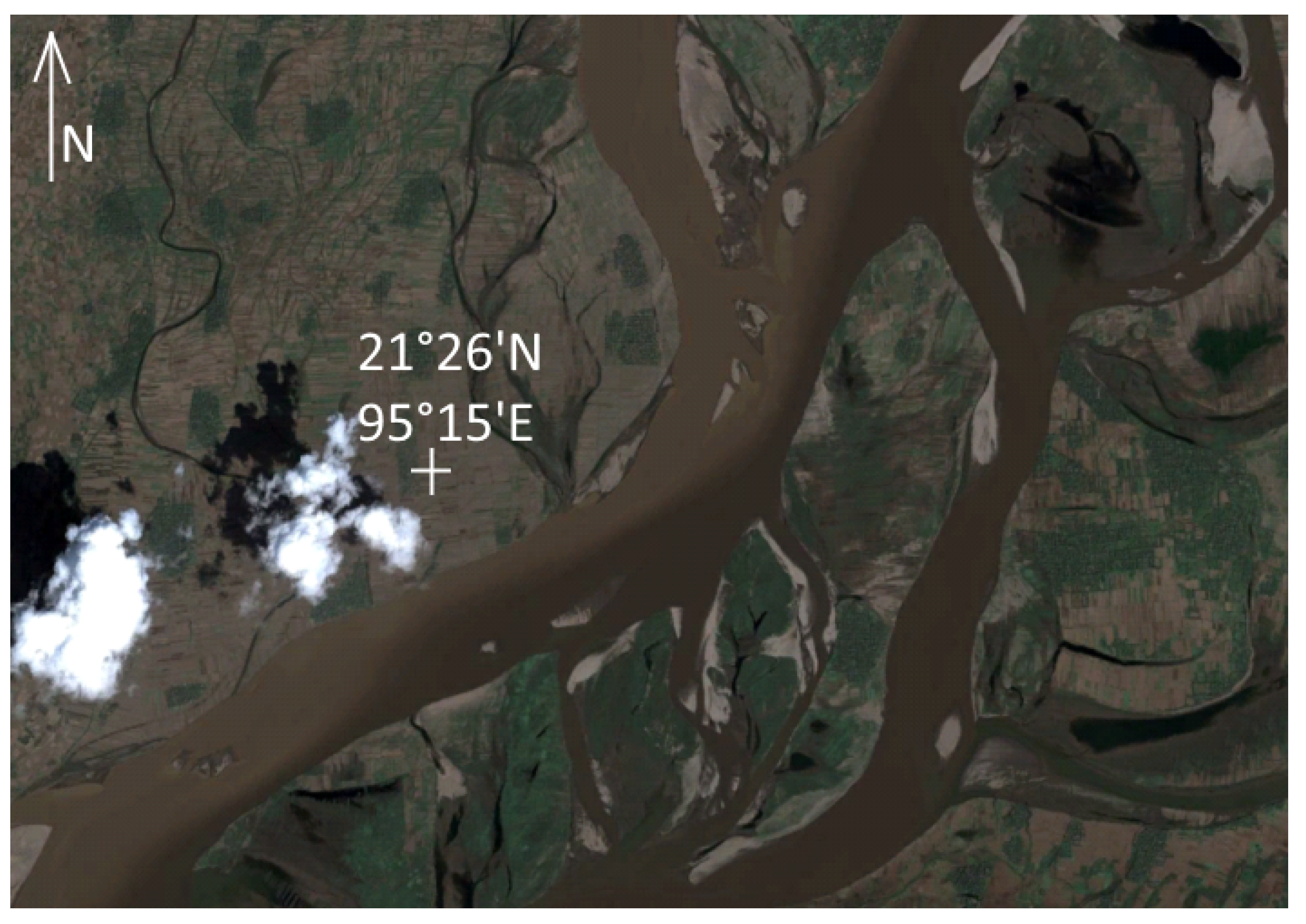
Aerial images of confluences with color differences can give us insight into the surface flow patterns downstream of the confluence. At the Chindwin–Irrawaddy confluence (Figure 3), we can for instance see that initially the denser and lighter colored water stemming from the Chindwin occupies the majority of the surface width. Further downstream, this shifts, and the lighter weight and darker colored Irrawaddy water occupies a larger portion of the river surface width. Moving even further downstream, the Chindwin water takes up a larger part of the surface width again. There are no coherent structures visible at the surface.
In a similar way, we can look at Figure 1A,B, showing aerial photographs of the Niger–Benue confluence in Nigeria. The lighter colored water from the Niger is denser than the darker Benue water. As noted in the introduction, the Benue water initially occupies the majority of the surface width (Figure 1A,B), while, more downstream, the Niger water occupies more (Figure 1A). Most downstream again the Benue water occupies most of the surface width (Figure 1A,B). In Figure 1A, there are no coherent structures visible, while, on Figure 1B, there are.
At the confluence of the Rhône and Arve (Figure 4), we see a different flow pattern. The denser Arve water rapidly reduces in abundance at the surface as we move in downstream direction. A little more downstream, it appears again along the opposite bank. The confluence angle for this confluence is zero, and the only appreciable bend is downstream of the area of interest, which makes this confluence very similar to the idealized confluence for the narrow river.
3.4. The Confluence of the SolimõEs and Rio Negro
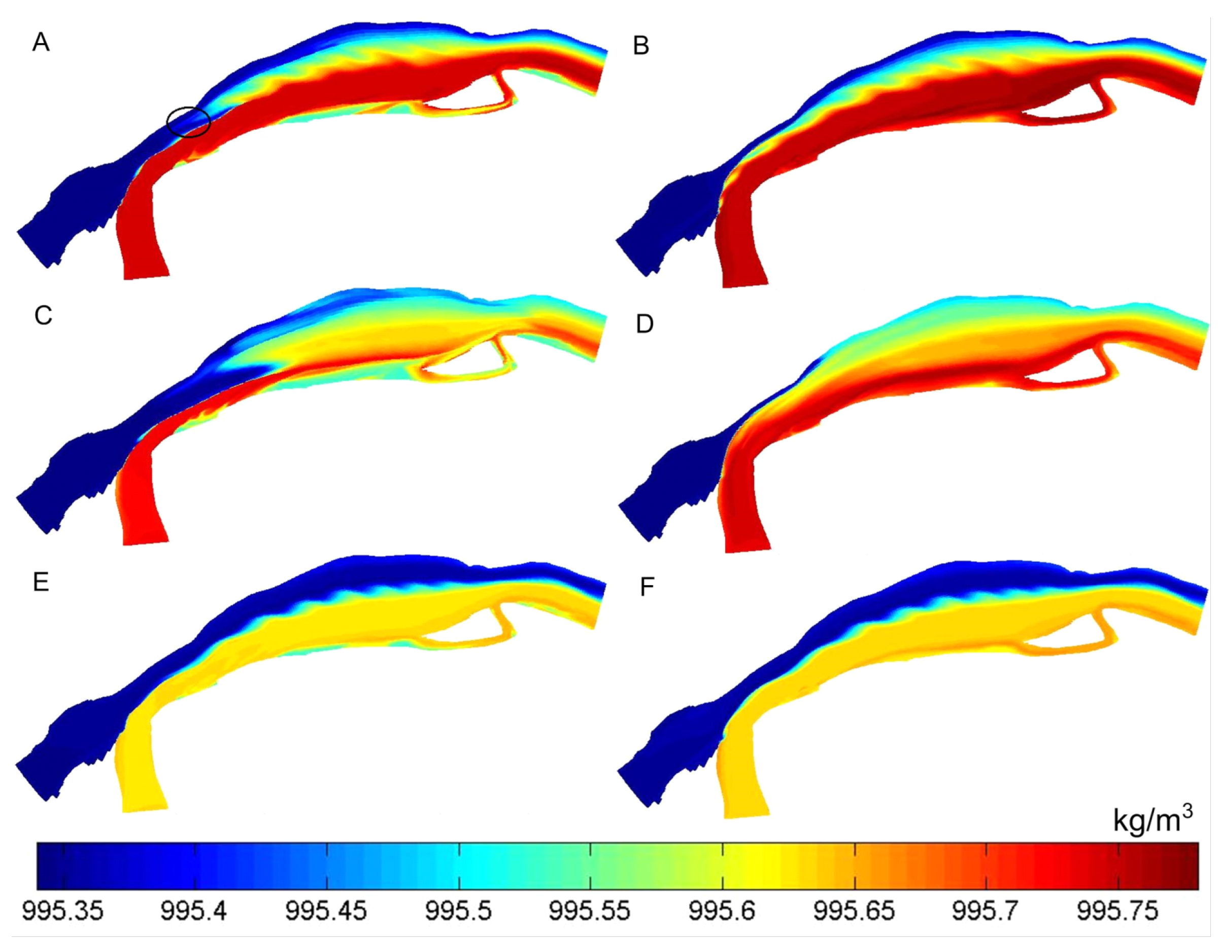
The results from the numerical hydrodynamic model of the confluence of the Rio Negro and Solimões rivers (Figure 11) show similar velocity distributions as measured in the field (cf. Reference [36]) and resemble the results from the idealized confluence (Figure 6). In both models, the denser water flowed under the lighter water, and the horizontal part of the interface moved upwards and eventually reached the surface. At the downstream end, complete mixing has not yet been achieved, which was also observed in this confluence by Park and Latrubesse [5] and in the idealized model. In both models, the development of coherent structures in the mixing layer was hampered, at least initially.
4. Discussion
4.1. Large-Scale Patterns
We found a large scale flow pattern occurring in confluences with a density difference between the tributaries, where the dense water flowed underneath the light water. Similar flow patterns were also reported for the confluences of the rivers Ebro and Segre [28] and Rio Negro and Solimões [33].
Besides this circulatory flow, we also identified a secondary large scale flow pattern. Here, the lower denser water progressively takes up a larger proportion of the depth when moving in downstream direction. This upward movement of the horizontal part of the interface can be explained from Schijf and Schönfelds [25] two-layer model:
Here, subscripts 1 and 2 refer to the top and bottom layer, respectively, d is the depth, u the velocity, q the constant discharge per unit width, the water density, x the streamwise coordinate, g the gravitational acceleration, the elevation of the bed, the shear stress on the interface between the two waters, and is the bed shear stress. In the last two equations, the sign of is opposite due to Newton’s third law (action = reaction).
The water in the top layer will accelerate if the second term of the third equation (describing the pressure gradient) is larger than the last term (describing the shear between the two layers). The first equation shows this will result in shallowing of the top layer. Usually, the pressure gradient is roughly compensated by bed friction [37]. Then, little acceleration or deceleration will occur. Since the shear between the two waters will be much smaller than the bed friction [23], the shear will also be much smaller than the pressure gradient. This theory thus predicts acceleration and shallowing of the light water near the surface. This explains the upward movement of the horizontal part of the shear layer.
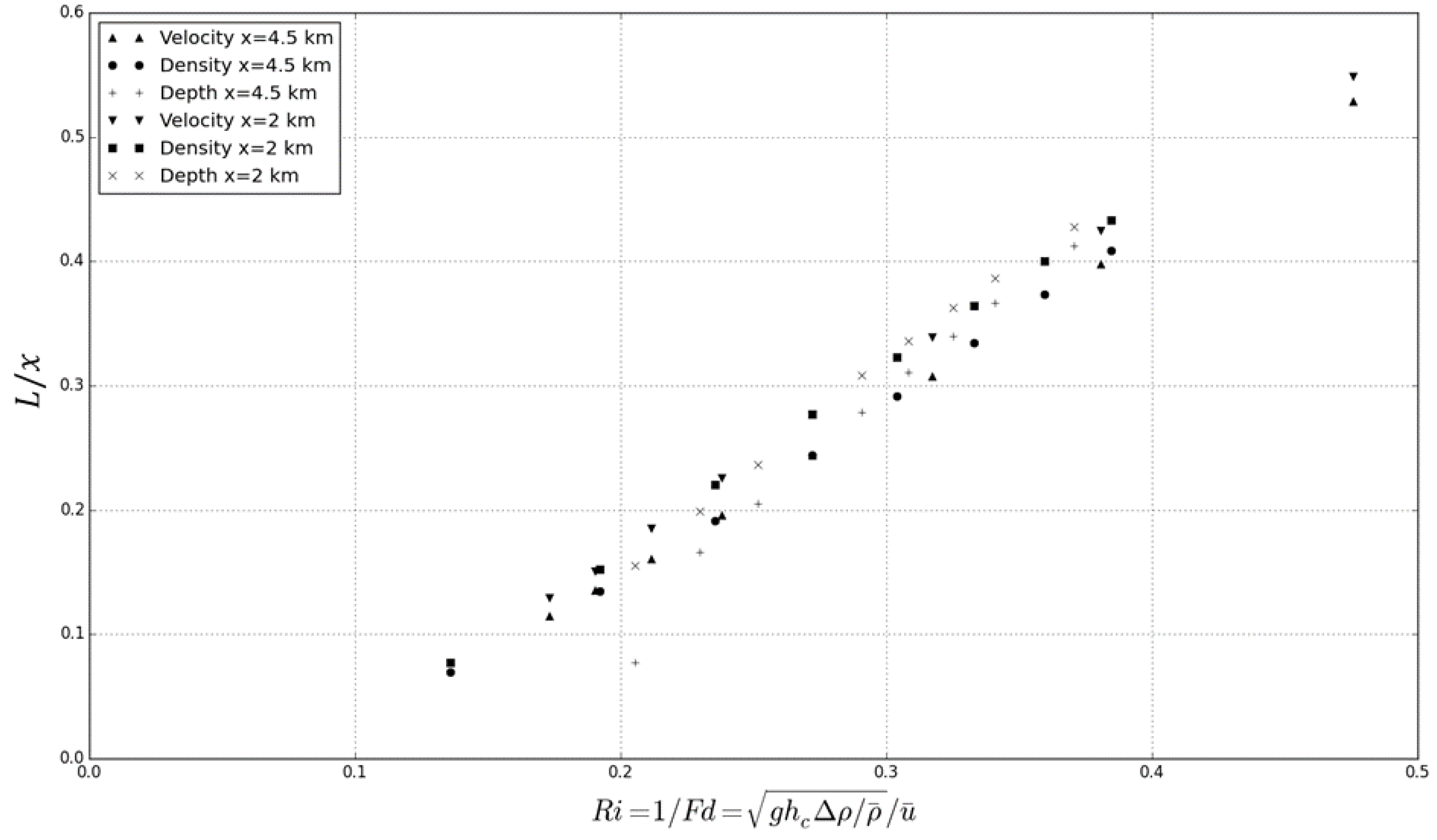
The strength of the first part of the large scale flow pattern: the circulation can be estimated by the velocities perpendicular to the main direction of flow [28], a non-dimensional form of which is the Richardson number. Figure 12 plots the length over which the two waters have flown over one another (L) divided by the downstream distance (x) as a function of the Richardson number. Every marker corresponds to one model run and a location either 2 or 4.5 km downstream of the confluence apex. The shape of the marker indicates the parameter setting that changed the Richardson number with respect to the base run. Since the water flows downstream with constant speed, the velocities perpendicular to the main flow can be estimated with L/x.
The circulation weakens slightly in downstream direction due to the changed height of the two density currents. All markers in Figure 12 pertaining to 2 km are above those of 4.5 km. This is caused by the upward shift of the interface, changing the heights of the density currents, which influences their speed [24]. All model runs represented in Figure 12 had a Chézy coefficient of 60 m0.5/s. Markers move downwards for higher friction and upwards for lower friction.
The rate at which the horizontal part of the interface between the two waters moves upwards is influenced by multiple parameters. At a higher roughness, the flow decelerates more strongly, and the interface reaches the surface sooner. The velocity difference influences the shear between the dense and light water. The interface will reach the surface later if the dense water flows faster than the light water, and sooner if the light water flows faster than the dense water. The model runs confirmed this.
4.2. Effect on the Mixing Layer
Velocity differences between two tributaries can produce a mixing layer. We showed that if also a density difference is present between the two tributaries, this mixing layer may not form. This is linked to how the coherent structures form. The coherent structures in the mixing layer have horizontal length scales much larger than the vertical length scale. They develop as rotating columns with a vertical axis of rotation. The density driven circular motion with axis in streamwise direction destroys these columns. Vermaas et al. [38] observed a similar secondary circulation of water hampering the development of coherent structures in flow over a bed with transverse roughness variations.
There was a clear relation between the combination of the Richardson number and the non-dimensional flow velocity difference and the presence of coherent structures around the shear layer. However, with different parametrizations leading to equal non-dimensional parameters, the coherent structures did not always grow to the same size. In none of our model runs did this lead to a different classification of the flow (coherent structures/no coherent structures/transitional). The difference in the size or hampering of the coherent structures is caused by the upwards movement of the interface between the two waters as it alters the velocity of the two density currents due to changing their heights. This makes the Richardson number at the confluence a weaker indicator of the strength of the circular water motion hampering the development of coherent structures.
As both non-dimensional parameters (Richardson number and non-dimensional velocity difference) have the flow velocity in the denominator, the non-dimensional parameter describes the slope of the lines in Figure 10. Coherent structures are present if the value of this parameter exceeds 3.4; no coherent structures are present if it is lower than 2.4. Possibly the bed roughness influences the exact value.
The instability condition of Daoyi and Jirka [22] could be added to Figure 10 by using the depth as the length scale for the stability number, S. The resulting number corresponds to a horizontal line in Figure 10 below which no coherent structures can develop, regardless of the Richardson number, but influenced by the bottom friction.
We identified that coherent structures are able to exist under larger density difference conditions than coherent structures closer to the top of the water column. Possibly structures at the bottom can exist longer because the weaker flows there hamper the development of coherent structures less.
It is worth emphasizing that none of the model runs with velocity differences had a width so small that the banks influenced the coherent structures. Therefore, we did not consider the complex flow field that might arise if coherent structures would reach one of the banks (cf. Reference [39]).
Although we have identified density difference effects on turbulent coherent structures downstream of a confluence, it is not yet possible to predict the amount of mixing downstream of a confluence. The spiraling fluid motion that hampers the development of coherent structures also increases the contact area between the two waters, which increases mixing. How much this process would increase mixing will depend on small-scale turbulence found around the interaction zone of the two waters.
How density differences and velocity differences affect the hydrodynamics downstream of a confluence is summarized in Figure 10, which pertains to the idealized cases we investigated. A more complete categorization of confluences might require considering helical flow cells due to flow realignment, helical flow cells due to bed discordance, confluence angles, and the width ratio of the tributaries. In many field studies, a combination of processes is taking place (cf. Reference [9,29]), and a categorical analysis based on non-dimensional parameters may be helpful in classifying which processes will be dominant.
4.3. Aerial Photographs
On aerial photographs of three river confluences, we identified flow patterns similar to the ones we identified in the idealized confluence. This indicates that it is likely that the same flow processes are occurring at these locations. Of course, the confluences of which we have found aerial photographs are different from the idealized confluence, which may have affected the water flow around this confluence.
In the Irrawaddy–Chindwin confluence (Figure 3), we, for instance, see a mild bend upstream of the confluence. As there are small islands downstream of the confluence which force the flows to realign before reaching the most downstream island, we assume this bend has little influence on the flow.
In the same confluence, we also find another bend more downstream in the area where the lighter-weight Irrawaddy water increases its occupation of the width. The curvature-induced helical flow in bends could shift the interface between the two waters at the surface [28]. This shift would be towards the outer bend. The opposite is observed, however, leading us to believe the density driven flow is, in this instance, stronger than the curvature induced flow.
The location of the shear layer can also be influenced by velocity differences between the tributaries. We can be certain that this has not a major effect on the identified flow at the Irrawaddy–Chindwin confluence, as well. This is because velocity differences would move the shear layer to one side, the side of the slower moving water [11,12]. Since the shear layer moves in both directions, this type of flow cannot explain the flow field, as seen in Figure 3.
In the numerical models, the light water always flowed over the denser water, causing it to occupy an increasingly larger proportion of the width at the surface. The semi-horizontal interface that then developed between the two waters moved upwards when moving in downstream direction. Eventually, it could reach the surface, causing the denser water to rapidly reoccupy a larger proportion of the width at the surface (Figure 7A). As this pattern is almost identical to what we see on the aerial photograph of the Chindwin–Irrawaddy confluence, we infer that the effect of density differences was significant at the Chindwin–Irrawaddy confluence for the time at which the aerial photograph was taken.
In addition, the two photographs of the Niger–Benue confluence (Figure 1) show similar features as the ones seen in the idealized confluence. Without any distinct bends and a small confluence angle this site looks similar to the idealized confluence. We can see two very different flow fields, however. Figure 1A shows that the Benue water occupies an increasingly larger part of the water surface in downstream direction, caused by the lighter-weight Benue water flowing over the denser Niger water. Further downstream the width of the Niger water at the surface increases again, similar to the result from the idealized model. Figure 1B does not show any increase in width of the lighter-weight Benue water at the surface. It shows, however, coherent structures developing in the mixing layer between the waters from the two tributaries, not present in Figure 1A. Figure 1A,B would thus need to be placed at different locations in Figure 10, with different values for the governing non-dimensional parameters. It is likely that, in Figure 1B, the Niger river is flowing faster than the Benue river. This velocity difference causes not only the coherent structures to develop, but it also causes the entire shear layer to shift towards the slower flow [11,12]. Although the two waters flow over one another, the lighter water at the surface does not widen due to the lateral shift of the entire shear layer. Both photographs show a widening of the denser water similar to that in the numerical model.
The confluence of the Rhône and Arve (Figure 4) is more similar to the case shown in Figure 8. We see the denser Arve water flow under the lighter Rhône water. It reaches the opposite bank where it wells up. This complies with the numerical simulations for the idealized confluence into a narrow river.
4.4. The Confluence of the SolimõEs and Rio Negro
The results obtained from the numerical model of the Solimões and Rio Negro confluence showed many similarities with the results of the idealized confluence. Actually, we can add markers (square) to Figure 10 pertaining to the three model runs for the Rio Negro-Solimões confluence. This shows that the amount of mixing may change in time, depending on the incoming flows, similar to what was found by Park and Latrubesse [5]. It is worth noting that Lane et al. [40] observed even stronger changes in mixing over time at the confluence of the Río Paraná and Río Paraguay, partly related to changing characteristics and partly to local topography.
In the numerical models and from Figure 10, we can see that coherent structures are absent at this confluence. Oblique photographs (like Figure 13) show the same. This seemed surprising as the velocity difference between the tributaries is always significant [32,41].
The oblique photograph (Figure 13), however, shows more: floating foam at the interface between the two waters. This indicates downwelling of denser water that dives under the lighter water (cf. Reference [42]). This is linked to the spiraling water motion that forms due to the density differences.
There were, however, also some differences between the model and the aerial photographs of the Rio Negro-Solimões confluence. In the model, a widening of the dense water at the surface was seen under some discharge conditions (Figure 11), which was not seen on the aerial photograph. This was because the water surface in the aerial photographs was disturbed by boils, as shown in Figure 14 where boils of Solimões water appear on the Rio Negro side of the river. The locations of the boils proved to be rather constant, forming lines. Therefore, we suppose the boils are similar to the ones described by Best (2005) and are generated at permanent bed anomalies. Ianniruberto et al. [43] found bed rock outcrops in this region, which could function as permanent bed anomalies.
The disturbance of the water surface by boils renders a widening of denser water at the surface unnoticeable as it is masked by the water transported to the surface by the boils. The boils were not reproduced by the numerical models because the grid cells were too large to resolve such processes. This process may also hamper the observation of possible coherent structures that develop downstream of it. Nonetheless, these boils do reveal the presence of denser Solimões water underneath the lighter Rio Negro water. This is in accordance with the numerical model and findings of previous research [36,41].
5. Conclusions
Our results show that small density differences caused by suspended sediment load or temperature differences can have a significant impact on the flow downstream of a confluence. Runs with the idealized numerical model demonstrated three important phenomena caused by the density difference between the tributaries:
- 1.
- The denser water flows under the lighter water. This results in widening of the light water at the surface. The shear layer will tilt and part of it will become almost horizontal. This horizontal part moves upwards and eventually reaches the surface, resulting further downstream in a decrease of the amount of light water at the surface.
- 2.
- If the downstream river is rather narrow, the two waters cannot keep flowing over one another. One or both of the waters will reach the opposite bank and start flowing up or down. Further downstream, only dense water may be present at the bank where initially only light water was present, and vice versa.
- 3.
- A difference in flow velocities between the tributaries can cause coherent structures to develop in the mixing layer. The movement of the water due to the density differences is perpendicular to the main flow direction. If this motion becomes too strong, it can hamper or even completely stop the development of coherent structures in the mixing layer. The occurrence of coherent structures in the mixing layer downstream of a confluence can be predicted by using two non-dimensional parameters, i.e., the Richardson number and the non-dimensional velocity difference. These parameters give an indication of the size of the disturbances in the mixing layer and the magnitude of the water motion due to the density differences.
These phenomena were visible not only in the numerical model but also on aerial photographs. The aerial photographs of the Niger–Benue (Figure 1A,B) and Irrawaddy–Chindwin (Figure 3) both show the widening of the lighter water at the surface followed further downstream by widening of the denser water of the surface. The aerial photograph of the Rhône–Arve confluence (Figure 4) showed that dense water can well up at the opposite bank if the downstream river is narrow. At the confluence of the Rio Negro and Solimões, the waters lacked mixing but widening and narrowing of the light water could not be distinguished because boils of dense Solimões water disturbed the water surface of the Rio Negro side of the river.
Most studies of the effects of density differences have focused on interactions between saline sea water and fresh water. The effects described in this study are caused by suspended sediment and temperature differences, for which the density differences are smaller. We found that even these small density differences can have major impacts. This demonstrates that density differences due to temperature, sediment concentration, or salinity should be included in any study where the hydro- or morphodynamics downstream of a confluence are of importance.
Other factors have an influence on confluence hydrodynamics, too. Examples are helical flow cells due to flow realignment, helical flow cells due to bed discordance, confluence angles, and the width ratio of the tributaries. We recommend further research to incorporate these factors into a general picture, along the lines of Figure 10.
Author Contributions
Conceptualization, E.v.R., E.M., and K.S.; methodology, E.v.R.; software, E.M. and K.S.; validation, E.v.R., E.M., and W.U.; formal analysis, E.v.R.; investigation, E.v.R.; resources, E.M., and K.S.; data curation, E.v.R.; writing—original draft preparation, E.v.R.; writing—review and editing, E.M. and W.U.; visualization, E.v.R. and E.M.; supervision, E.M., K.S., and W.U.; project administration, E.M. and K.S. All authors have read and agreed to the published version of the manuscript.
Funding
This research received no external funding.
Acknowledgments
We would like to thank Rob Uittenbogaard. Without him, the HLES module would not have performed as it did. We would like to thank Jim Best for his advice, which greatly improved the quality of this paper.
Conflicts of Interest
The authors declare no conflict of interest.
References
- Ardura, A.; Gomes, V.; Linde, A.R.; Moreira, J.C.; Horreo, J.L.; Garcia-Vazquez, E. The Meeting of Waters, a possible shelter of evolutionary significant units for Amazonian fish. Conserv. Genet. 2013, 14, 1185–1192. [Google Scholar] [CrossRef]
- Gualtieri, C.; Abdi, R.; Ianniruberto, M.; Filizola, N.; Endreny, T.A. A 3D analysis of spatial habitat metrics about the confluence of Negro and Solimões rivers, Brazil. Ecohydrology 2019, e2166. [Google Scholar] [CrossRef]
- Best, J.L. Flow dynamics at river channel confluences: Implications for sediment transport and bed morphology. SEPM 1987. [Google Scholar] [CrossRef]
- Best, J.L.; Reid, I. Separation zone at open-channel junctions. J. Hydraul. Eng. 1984, 110, 1588–1594. [Google Scholar] [CrossRef]
- Park, E.; Latrubesse, E.M. Surface water types and sediment distribution patterns at the confluence of mega rivers: The Solimões-Amazon and Negro Rivers junction. Water Resour. Res. 2015, 51, 6197–6213. [Google Scholar] [CrossRef]
- Biron, P.M.; Richer, A.; Kirkbride, A.D.; Roy, A.G.; Han, S. Spatial patterns of water surface topography at a river confluence. Earth Surf. Process. Landf. 2002, 27, 913–928. [Google Scholar] [CrossRef]
- Rhoads, B.L.; Kenworthy, S.T. Flow structure at an asymmetrical stream confluence. Geomorphology 1995, 11, 273–293. [Google Scholar] [CrossRef]
- Rhoads, B.L.; Sukhodolov, A.N. Field investigation of three-dimensional flow structure at stream confluences: 1. Thermal mixing and time-averaged velocities. Water Resour. Res. 2001, 37, 2393–2410. [Google Scholar] [CrossRef]
- Riley, J.D.; Rhoads, B.L.; Parsons, D.R.; Johnson, K.K. Influence of junction angle on three-dimensional flow structure and bed morphology at confluent meander bends during different hydrological conditions. Earth Surf. Process. Landf. 2015, 40, 252–271. [Google Scholar] [CrossRef]
- Bradbrook, K.F.; Lane, S.N.; Richards, K.S. Numerical simulation of three-dimensional, time-averaged flow structure at river channel confluences. Water Resour. Res. 2000, 36, 2731–2746. [Google Scholar] [CrossRef] [Green Version]
- Kirkil, G. Flow structure in a mixing layer developing over a flat bed at high Reynolds numbers. In Proceedings of the E-Proceedings of the 36th IAHR World Congress, The Hague, The Netherlands, 28 June–3 July 2015. [Google Scholar]
- Uijttewaal, W.S.J.; Tukker, J. Development of quasi two-dimensional structures in a shallow free-surface mixing layer. Exp. Fluids 1998, 24, 192–200. [Google Scholar] [CrossRef]
- Biron, P.; Roy, A.; Best, J.L.; Boyer, C.J. Bed morphology and sedimentology at the confluence of unequal depth channels. Geomorphology 1993, 8, 115–129. [Google Scholar] [CrossRef]
- Biron, P.M.; Ramamurthy, A.S.; Han, S. Three-dimensional numerical modeling of mixing at river confluences. J. Hydraul. Eng. 2004, 130, 243–253. [Google Scholar] [CrossRef]
- Biron, P.; Best, J.L.; Roy, A.G. Effects of bed discordance on flow dynamics at open channel confluences. J. Hydraul. Eng. 1996, 122, 676–682. [Google Scholar] [CrossRef]
- van Prooijen, B.C.; Uijttewaal, W.S.J. A linear approach for the evolution of coherent structures in shallow mixing layers. Phys. Fluids 2002, 12, 4105–4114. [Google Scholar] [CrossRef] [Green Version]
- Konsoer, K.M.; Rhoads, B.L. Spatial-temporal structure of mixing interface turbulence at two large river confluences. Environ. Fluid Mech. 2014, 14, 1043–1070. [Google Scholar] [CrossRef]
- Constantinescu, G.; Miyawaki, S.; Rhoads, B.; Sukhodolov, A. Numerical analysis of the effect of momentum ratio on the dynamics and sediment-entrainment capacity of coherent flow structures at a stream confluence. J. Geophys. Res. Earth Surf. 2012, 117. [Google Scholar] [CrossRef]
- Herrero, H.S.; García, C.M.; Pedocchi, F.; López, G.; Szupiany, R.N.; Pozzi-Piacenza, C.E. Flow structure at a confluence: Experimental data and the bluff body analogy. J. Hydraul. Res. 2016, 54, 263–274. [Google Scholar] [CrossRef]
- Miyawaki, S.; Constantinescu, G.; Rhoads, B.; Sukhodolov, A. Changes in three-dimensional flow structure at a river confluence with changes in momentum ratio. River Flow 2010, 225–232. [Google Scholar]
- Best, J.L.; Roy, A.G. Mixing-layer distortion at the confluence of channels of different depth. Nature 1991, 350, 411–413. [Google Scholar] [CrossRef]
- Daoyi, C.; Jirka, G.H. Linear stability analysis of turbulent mixing layers and jets in shallow water layers. J. Hydraul. Res. 1998, 36, 815–830. [Google Scholar] [CrossRef]
- Vreugdenhil, C.B. Computation of Gravity Currents in Estuaries; TU Delft: Delft, The Netherlands, 1970. [Google Scholar]
- Shin, J.O.; Dalziel, S.B.; Linden, P.F. Gravity currents produced by lock exchange. J. Fluid Mech. 2004, 521, 1–34. [Google Scholar] [CrossRef] [Green Version]
- Schijf, J.B.; Schönfled, J.C. Theoretical considerations on the motion of salt and fresh water. In Proceedings of the Minnesota International Hydraulic Convention, IAHR, Minneapolis, MN, USA, 1–4 September 1953. [Google Scholar]
- Cook, C.B.; Richmond, M.C. Monitoring and simulating 3-D density currents at the confluence of the snake and clearwater rivers. Crit. Transit. Water Environ. Resour. Manag. 2004, 1–9. [Google Scholar] [CrossRef]
- Lyubimova, T.; Lepikhin, A.; Konovalov, V.; Parshakova, Y.; Tiunov, A. Formation of the density currents in the zone of confluence of two rivers. J. Hydrol. 2014, 508, 328–342. [Google Scholar] [CrossRef]
- Ramón, C.L.; Armengol, J.; Dolz, J.; Prats, J.; Rueda, F.J. Mixing dynamics at the confluence of two large rivers undergoing weak density variations. J. Geophys. Res. Oceans 2014, 119, 2386–2402. [Google Scholar] [CrossRef]
- Lewis, Q.W.; Rhoads, B.L. Rates and patterns of thermal mixing at a small stream confluence under variable incoming flow conditions. Hydrol. Process. 2015, 29, 4442–4456. [Google Scholar] [CrossRef]
- Deltares. Delft3D-FLOW, Simulation of Multi-Dimensional Hydrodynamic Flows and Transport Phenomena, Including Sediments: User Manual; Deltares: Delft, The Netherlands, 2014. [Google Scholar]
- Booij, R.; Tukker, J. Integral model of shallow mixing layers. J. Hydraul. Res. 2001, 36, 169–179. [Google Scholar] [CrossRef]
- ANA. Hidroweb. Available online: http://www.hidroweb.ana.gov.br/default.asp (accessed on 12 June 2016).
- Laraque, A.; Guyot, J.L.; Filizola, N. Mixing processes in the Amazon River at the confluences of the Negro and Solimoes Rivers, Encontro das Aguas, Manaus, Brazil. Hydrol. Process. 2009, 23, 3131–3140. [Google Scholar] [CrossRef]
- Trevethan, M.; Martinelli, A.; Oliveira, M.; Ianniruberto, M.; Gualtieri, C. Fluid mechanics, sediment transport and mixing about the confluence of Negro and Solimoes Rivers, Manaus, Brazil. In Proceedings of the 36th IAHR World Congress, The Hague, The Netherlands, 28 June–3 July 2015. [Google Scholar]
- Richey, J.E.; Meade, R.H.; Salati, E.; Devol, A.H.; Nordin, C.F.; Santos, U.D. Water discharge and suspended sediment concentrations in the Amazon River: 1982–1984. Water Resour. Res. 1986, 22, 756–764. [Google Scholar] [CrossRef]
- Gualtieri, C.; Filizola, N.; De Oliveira, M.; Santos, A.M.; Ianniruberto, M. A field study of the confluence between Negro and Solimões Rivers. Part 1: Hydrodynamics and sediment transport. Comptes Rendus Geosci. 2018, 350, 31–42. [Google Scholar] [CrossRef]
- Chow, V.T. Chapter 5. In Open-Channel Hydraulics; McGraw-Hill Book Company: New York, NY, USA, 1959; Volume 1, pp. 89–114. [Google Scholar]
- Vermaas, D.A.; Uijttewaal, W.S.J.; Hoitink, A.J.F. Lateral transfer of streamwise momentum caused by a roughness transition across a shallow channel. Water Resour. Res. 2011, 47. [Google Scholar] [CrossRef]
- van Heijst, G.F.J.; Clercx, H.J.H.; Molenaar, D. The effects of solid boundaries on confined two-dimensional turbulence. J. Fluid Mech. 2006, 554, 411–431. [Google Scholar] [CrossRef]
- Lane, S.N.; Parsons, D.R.; Best, J.L.; Orfeo, O.; Kostaschuk, R.A.; Hardy, R.J. Causes of rapid mixing at a junction of two large rivers: Río Paraná and Río Paraguay, Argentina. J. Geophys. Res. Earth Surf. 2008, 113. [Google Scholar] [CrossRef] [Green Version]
- Filizola, N.; Spínola, N.; Arruda, W.; Seyler, F.; Calmant, S.; Silva, J. The Rio Negro and Rio Solimões confluence point–hydrometric observations during the 2006/2007 cycle. In River, Coastal and Estuarine Morphodynamics: RCEM 2009; Taylor & Francis Group: Boca Raton, FL, USA, 2009; pp. 1003–1006. [Google Scholar]
- O’Donnel, J.; Marmorino, G.O.; Trump, C.L. Convergence and Downwelling at a River Plume Front. J. Phys. Oceanogr. 1998, 28, 1481–1495. [Google Scholar] [CrossRef]
- Ianniruberto, M.; Trevethan, M.; Pinheiro, A.; Andrade, J.F.; Dantas, E.; Filizola, N.; Santos, A.; Gualtieri, C. A field study of the confluence between Negro and Solimões Rivers. Part 2: Bed morphology and stratigraphy. Comptes Rendus Geosci. 2018, 350, 43–54. [Google Scholar] [CrossRef]
Figure 1.
Aerial photographs of the Niger–Benue confluence on (A) 5 December 2011 and (B) 21 December 2005. Flows are from top to bottom. The lighter colored Niger water is on the left, and the darker colored Benue water on the right. Source: Google Earth (edited).
Figure 1.
Aerial photographs of the Niger–Benue confluence on (A) 5 December 2011 and (B) 21 December 2005. Flows are from top to bottom. The lighter colored Niger water is on the left, and the darker colored Benue water on the right. Source: Google Earth (edited).

Figure 2.
Drawing of a cross-section, with dense water flowing over light water and the definition of L.
Figure 2.
Drawing of a cross-section, with dense water flowing over light water and the definition of L.

Figure 3.
Aerial photograph of the Chindwin–Irrawaddy confluence on 26 October 2009. Flows are from top to bottom. Source: Google Earth (edited).
Figure 3.
Aerial photograph of the Chindwin–Irrawaddy confluence on 26 October 2009. Flows are from top to bottom. Source: Google Earth (edited).

Figure 4.
Aerial photograph of the Rhône-Arve confluence near Geneva (Switzerland) on 1 July 2009. Flows are from right to left. Source: Google Earth (edited).
Figure 4.
Aerial photograph of the Rhône-Arve confluence near Geneva (Switzerland) on 1 July 2009. Flows are from right to left. Source: Google Earth (edited).

Figure 5.
Map showing the locations of the studied confluences, with zoomed in maps for each confluence.
Figure 5.
Map showing the locations of the studied confluences, with zoomed in maps for each confluence.

Figure 6.
Density profiles in the base run simulation. (A) Top view. (B) Longitudinal cross-section (C–E) Cross sections. Locations of (B–E) shown in (A).
Figure 6.
Density profiles in the base run simulation. (A) Top view. (B) Longitudinal cross-section (C–E) Cross sections. Locations of (B–E) shown in (A).

Figure 7.
Conceptual picture of the shape of the interface between dense and light water without a velocity difference. The arrows indicate the flow direction and the side where the dense (dark) and light (light) waters enter the confluence area. (A) A wide downstream channel (B) a narrow downstream channel.

Figure 8.
Densities in the top and bottom layer in the case with half the width, such that the width becomes restrictive.
Figure 8.
Densities in the top and bottom layer in the case with half the width, such that the width becomes restrictive.

Figure 9.
(A) Top view of the base scenario where the different colors indicate different densities. (red = dense, blue = light) Flow from left to right. (B) Same view for a situation with 1/4 of the density difference.
Figure 9.
(A) Top view of the base scenario where the different colors indicate different densities. (red = dense, blue = light) Flow from left to right. (B) Same view for a situation with 1/4 of the density difference.

Figure 10.
Diagram showing combinations of Richardson number and non-dimensional velocity difference for which coherent structures may or may not develop. Every marker represents one or more model runs, and the shape and color of the marker indicates the occurrence or non-occurrence of coherent structures. The values for the Rio Negro–Solimões model runs (Table 2) are also included.

Figure 11.
The density profiles in the Rio Negro–Solimões model runs. (A) Highest momentum ratio, top layer. (B) Highest momentum ratio, bottom layer. (C) Low flow, top layer. (D) Low flow, bottom layer. (E) High flow, top layer. (F) High flow, bottom layer.
Figure 11.
The density profiles in the Rio Negro–Solimões model runs. (A) Highest momentum ratio, top layer. (B) Highest momentum ratio, bottom layer. (C) Low flow, top layer. (D) Low flow, bottom layer. (E) High flow, top layer. (F) High flow, bottom layer.

Figure 12.
The relationship between the dimensionless amount of overturning and the Richardson number at 2 and 4.5 km downstream of the confluence apex.
Figure 12.
The relationship between the dimensionless amount of overturning and the Richardson number at 2 and 4.5 km downstream of the confluence apex.

Figure 13.
Oblique aerial photograph of the confluence of the Solimões and Rio Negro. Source: http://www.panoramio.com/photo/90000345.
Figure 13.
Oblique aerial photograph of the confluence of the Solimões and Rio Negro. Source: http://www.panoramio.com/photo/90000345.

Figure 14.
Boils of Solimões water on the Rio Negro side of the river. The markers show the most upstream locations of the boils for the available aerial photographs. Location shown in Figure 11A.
Figure 14.
Boils of Solimões water on the Rio Negro side of the river. The markers show the most upstream locations of the boils for the available aerial photographs. Location shown in Figure 11A.


Table 1.
Overview of the model runs and the parameter values used therein. The bold numbers relate to the basecase scenario and are the values used if no other value is reported.
Table 1.
Overview of the model runs and the parameter values used therein. The bold numbers relate to the basecase scenario and are the values used if no other value is reported.
| Velocity Ratio | |||||||||
|---|---|---|---|---|---|---|---|---|---|
| Parameter | 3/7 | 7/13 | 2/3 | 9/11 | 1 | 11/9 | 3/2 | 13/7 | 7/3 |
| Bed level (m) | −20, −25, −30, −35, −40, −45, −55, −60, −65 | 17.5, −35 | −17.5, −35 | −17.5, −25, −35, −52.5 | |||||
| Temperature difference ( C) | 0.5, 1, 1.5, 2, 2.5, 3, 3.5, 4 | 0.5, 1, 2 | 0.5, 1, 2, 2.5 | 0.5, 1, 2, 2.5, 3 | |||||
| Mean temperature (C) | 30 | ||||||||
| Mean flow velocity (m/s) | 0.676, 0.845, 1.014, 1.183, 1.352, 1.521, 1.690, 1.859 | ||||||||
| Chézy roughness (m0.5/s) | 40, 50, 60, 70, 80 | ||||||||
| Grid cells (n × n) | 1000 × 81, 1000 × 161 | ||||||||
| Turbulence model | k- | ||||||||
| Number of -layers | 20 |
Table 2.
Overview of parameters used in the model runs for the Solimões–Rio Negro confluence model.
| Discharge (m3/s) 1 | Temperature (C) | Sediment Concentration (kg/m3) | ||||
|---|---|---|---|---|---|---|
| Rio Negro | Solimões | Rio Negro | Solimões | Rio Negro | Solimões | |
| High Flow | 70,000 | 120,000 | 31 2 | 30.4 2 | 0 | 0.160 |
| Highest Momentum ratio | 30,000 | 100,000 | 31 2 | 30.4 2 | 0 | 0.345 |
| Low flow | 25,000 | 60,000 | 31 3 | 30.4 3 | 0 | 0.321 |
Based on ANA (2016), Estimated, no data found, Based on Laraque et al. (2009) and Trevethan et al. (2015), Based on Richey et al. (1986).
Publisher’s Note: MDPI stays neutral with regard to jurisdictional claims in published maps and institutional affiliations. |
© 2020 by the authors. Licensee MDPI, Basel, Switzerland. This article is an open access article distributed under the terms and conditions of the Creative Commons Attribution (CC BY) license (http://creativecommons.org/licenses/by/4.0/).
Share and Cite
MDPI and ACS Style
van Rooijen, E.; Mosselman, E.; Sloff, K.; Uijttewaal, W. The Effect of Small Density Differences at River Confluences. Water 2020, 12, 3084. https://doi.org/10.3390/w12113084
AMA Style
van Rooijen E, Mosselman E, Sloff K, Uijttewaal W. The Effect of Small Density Differences at River Confluences. Water. 2020; 12(11):3084. https://doi.org/10.3390/w12113084
Chicago/Turabian Stylevan Rooijen, Erik, Erik Mosselman, Kees Sloff, and Wim Uijttewaal. 2020. "The Effect of Small Density Differences at River Confluences" Water 12, no. 11: 3084. https://doi.org/10.3390/w12113084
Note that from the first issue of 2016, this journal uses article numbers instead of page numbers. See further details here.