Article

Comparison between Periodic Tracer Tests and Time-Series Analysis to Assess Mid- and Long-Term Recharge Model Changes Due to Multiple Strong Seismic Events in Carbonate Aquifers

1
Dipartimento SIMAU, Università Politecnica delle Marche, Via Brecce Bianche 12, 60122 Ancona, Italy
2
Dipartimento di Ingegneria e Geologia (InGeo), Università “G. d’Annunzio” Chieti-Pescara, Via dei Vestini 30, 66013 Chieti, Italy
3
Dipartimento di Fisica e Geologia, Università di Perugia, Via Pascoli snc, 06123 Perugia, Italy
*
Author to whom correspondence should be addressed.
Water 2020, 12(11), 3073; https://doi.org/10.3390/w12113073
Submission received: 28 September 2020 / Revised: 26 October 2020 / Accepted: 28 October 2020 / Published: 2 November 2020

Abstract

:
Understanding the groundwater flow in carbonate aquifers represents a challenging aspect in hydrogeology, especially when they have been struck by strong seismic events. It has been proved that large earthquakes change springs hydrodynamic behaviour showing transitory or long-lasting variations and making their management much more difficult. This is the case of Sibillini Massif (central Italy), which has been hit by the well-known 2016–2017 seismic period. This work aims to improve the knowledge of carbonate aquifers groundwater circulation and their possible changes in the hydrodynamic behaviour, during and after a series of strong seismic events. The goal has been achieved by comparing long-time tracer tests and transient time-series analysis, based on a sliding-window approach. This approach allowed investigating transient variations in the carbonate aquifers recharge system, highlighting the changes of relationships between the inflow contributions to the spring discharge in the area. As a result, the seismically triggered pore pressure distribution, and the hydraulic conductivity variations, because of the ground shaking and the fault systems activation, account for all the mid- and long-term modifications in the recharge system of Sibillini aquifers, respectively. These outcomes provide valuable insights to the knowledge of aquifer response under similar hydrogeological conditions, that are vital for water management.

1. Introduction

Transitory or permanent changes in hydrodynamic behaviour due to a series of strong seismic events are known all over the world [1,2,3,4,5]. Many authors tried to understand and explain which processes are responsible for the hydrogeological modification after big earthquakes [6,7,8,9]. For instance, Koizumi et al. [10] analysed streamflow data from eight observation stations on three major rivers in Kumamoto Prefecture and they surveyed 11 water springs in the region several times after the main shock (Mw 7.3), which occurred in Kumamoto Prefecture, Japan. Some of the eight observation stations recorded large increases in streamflow following a heavy rainfall that occurred two months after the earthquake. They supposed that this effect could be associated with a decrease in the water-holding capacity of the catchment caused by earthquake-induced landslides but the earthquake-related changes in the spring flow rate were not so clear.
In Italy, Amoruso et al. [11] proposed a conceptual model of the earthquake consequences on the Gran Sasso aquifer due to the L’Aquila earthquake (Mw 6.3). In this model, the short-term hydrologic effects registered, immediately after the main shock, were determined to have been caused by a pore pressure increase related to aquifer deformation, while the mid-term effects highlighted a change in groundwater hydrodynamics. They suggested that supplementary groundwater that flows towards aquifer boundaries and springs in discharge areas reflects a possible increase in hydraulic conductivity in the recharge area, nearby the earthquake fault zone.
Valigi et al. [12] investigated a significant discharge alteration to the Pescara di Arquata spring (exploited for drinking purposes), due to the 24 August 2016 (Mw 6.0) extensional Amatrice earthquake and to 30 October 2016 (Mw 6.5) Norcia event. They argued that the increase in post-seismic depletion coefficients indicates that the aquifer empties faster than it did during the inter-seismic period. The observed transient increase and subsequent decrease of discharge were consistent with a transient earthquake-related increase in hydraulic conductivity.
The extremely high heterogeneity and complexity of the aquifers are linked to the different types of porosity as well as their distribution throughout the subsoil [13,14], that affect the groundwater flow; thus, they represent an important challenge for hydrogeologists, who try to get a deeper insight into the hydrodynamic features under different conditions. The comprehension of such features is much more difficult when the system is affected by an external modification influencing the hydrodynamic response of springs fed by these aquifers. The latter is the case of a large earthquake or a series of strong seismic events that may modify the porosity of the system [15]. An increasing or decreasing of the permeability or a possible change of the aquifer geometry can also modify the groundwater circulation and flow paths, making water resource management a real challenge.
From a methodological point of view, these issues are increasingly addressed also by time-series analysis and tracer tests. The former is used to highlight the correlation between recharge processes and discharge [16,17,18,19], whereas the latter is used to identify the preferential flow path in aquifers and potential connections and exchanges among hydro-structures [20,21] and to determine the aquifer characteristics [22].
In this study, the Sibillini carbonate Massif (central Italy) was investigated. That area has been selected due to several Mw > 5.0 earthquakes during the 2016–2017 seismic period [23] which affected its groundwater circulation [24]. According to [25], after the main shock (Mw 6.5, 30 October 2016), the springs located on the eastern and southern-eastern side of the massif shown a long-lasting decrease in discharge values, meanwhile the springs and rivers located westward shown an increase in discharge values [26,27]. Although many efforts were made to propose a preliminary conceptual model of the water circulation after the seismic events [28], a study which aims to investigate the time response of springs discharge to the rainfall and/or snowfall in the system has not yet been conducted. For this purpose, a transient time-series analysis, made via a Sliding-Window Cross-Correlation Function (SWCCF) between the inflow (i.e., rainfall, snowfall) and outflow (i.e., discharge), has been performed on three springs of the study area. The time-series analysis has been compared with two long time tracer tests conducted in 2018 and 2019, after the seismic events, and to the others conducted before in the same area [29]. In particular, this work is aimed to investigate the recharge system in a carbonate aquifer and to assess its changes caused by a series of strong seismic events.

2. Materials and Methods
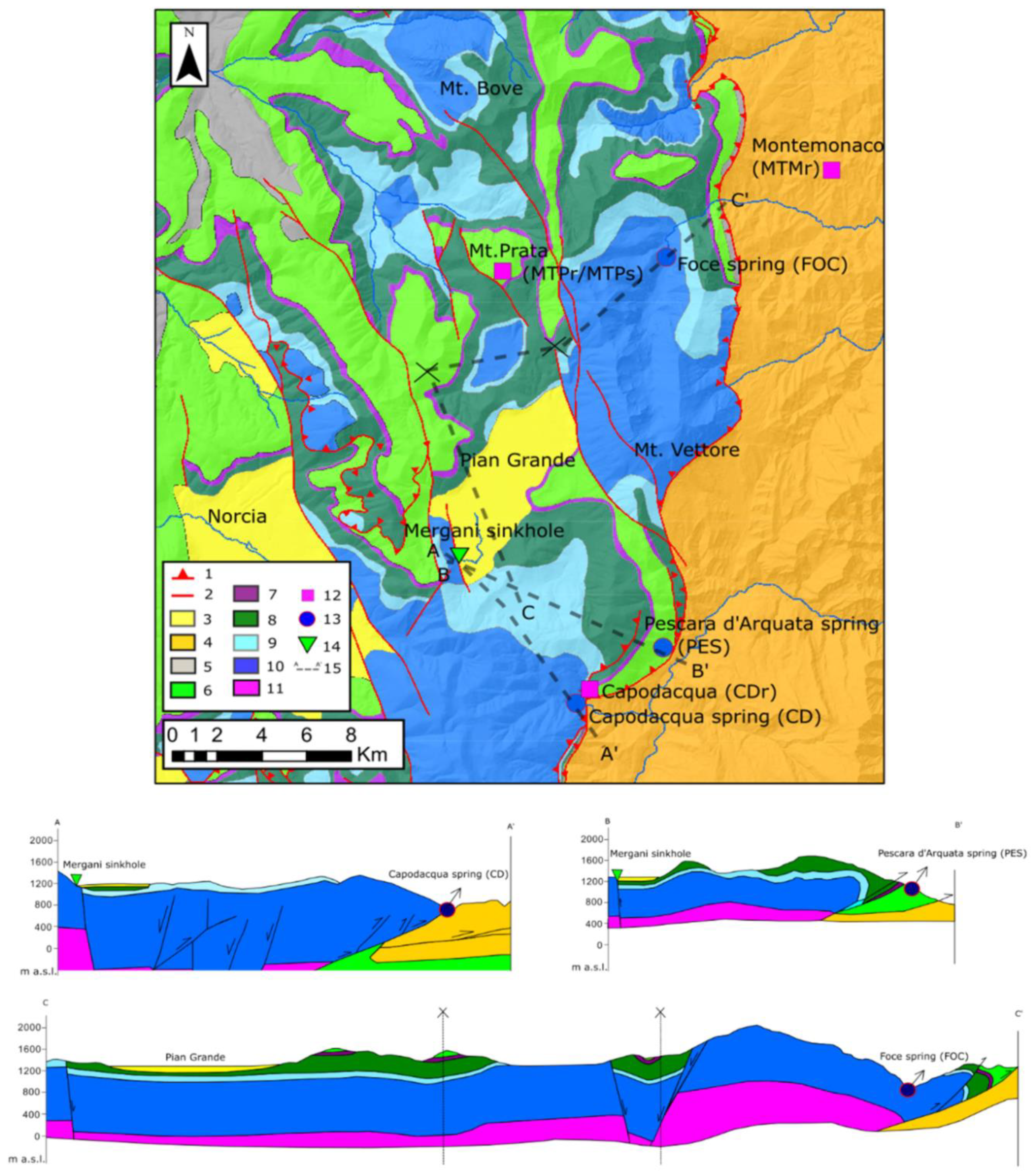
2.1. Study Area

The study area is located in central Italy and involves the carbonate sequence of Sibillini Massif (Figure 1). The hydrogeological setting of the area is strictly influenced by the stratigraphic and the tectonic features [30,31,32]. The so-called Basal aquifer is hosted by the Calcare Massiccio and Corniola formations (Upper Triassic-Lower Jurassic), a carbonate platform disarticulated in different domains characterised by a well-developed karstic system [29,33]. This is locally separated by the Upper Jurassic aquiclude (Calcareous siliceous marly units) from the Maiolica aquifer mainly composed of stratified micritic limestone, characterised by fissure and only partially by the minor karstic system. The latter is separated by the Scaglia Calcarea (stratified and fissured limestone) aquifer by the regional Marne a Fucoidi aquiclude (Figure 1). Before the seismic events, the Basal aquifer, which feeds the principal springs of the domain, was characterised by a prevalent circulation directed SSE-NNW (Apennine direction) according to the tectonic setting [34,35,36,37].
However, the fault system was responsible for local groundwater exchanges between different sectors of the aquifer (transversal direction) [28,29]. The Maiolica aquifer, when separated by the Basal one and the Scaglia Calcarea aquifer, is responsible for local groundwater recharge through the minor springs of the area [39]. After the seismic events, the transversal exchanges between the different hydro-structures seem to be more developed towards the western sector of the domain, while the Apennine flow direction (SSE-NNW) still characterise the Basal aquifer. According to the literature [29,39], the hydrogeological boundaries of the Sibillini Massif are represented in the eastern and southern-east portion of the domain by the Sibillini overthrust, while the western boundary is represented by the Nottoria-Preci normal fault system. As concerns the northern hydrogeological boundary, its features have not been clearly defined in literature yet [29]. However, according to the structural framework characterised by a general immersion of the fold axes towards the NW [35], the Nera River can be identified as the main area of groundwater preferential flow.
In a barycentric position with respect to the study area, there is the Pian Grande plain, which represents a large plateau located almost 1300 m a.s.l. This plain is a tectono-karstic basin filled by Holocenic lacustrine deposits in which several sinkholes are located [29]; the main one, named the Mèrgani sinkhole, has been instrumented by a hydrometric station and starting from 2017 a continuously daily discharge inflowing in the sinkhole has been recorded.

2.2. Datasets

In Table 1, all the details of the monitoring network are shown.
The three selected discharge monitoring points are located radially with respect to the Pian Grande plain, in the eastern and southern east portion of the massif (Figure 1). Pescara springs (PES, at 926 m a.s.l.) and Capodacqua (CD, at 841 m a.s.l.) are located in the southern part of the domain, while Foce spring (FOC) is located eastward, at 910 m a.s.l. For all the monitoring points the daily discharge data are available and provided by the drinking water company CIIP S.p.A. The spring discharge has been measured through water level sensors located in a specific weir with rectangular sections, which have an accuracy of ±5 % for PES, ±1.9 % for CD, and ±1.5 % for FOC. Three rain gauges and one snow thickness gauge, managed by Civil Protection Agency (Marche Region), have been selected to measure the meteo-climatic conditions of the area. In particular, Monte Prata rain (MTPr) and snow cover thickness (MTPs) gauge, located at 1813 m a.s.l., has been used to represent and analyse the main meteorological contribution from the highest portion of the massif, which represents the main recharge areas for the analysed springs; while Montemonaco (MTMr) and Capodacqua (CDr) rain gauges were used to measure the local meteorological condition, nearby the considered springs. The rain gauge and the snow thickness gauge daily data are available online at (https://www.regione.marche.it/Regione-Utile/Protezione-Civile/Console-Servizi-Protezione-Civile/SIRMIP-online). Due to its barycentric position and its inflow in the hydrogeological system, MGS was selected as an artificial-tracer injection point. For this purpose, many tracer tests were performed to investigate the hydrodynamics of the area [29,40]. Not least, in this work, two tracer tests conducted about 2 and 3 years after the seismic events, were compared by the others conducted by Nanni et al. [29] in 2016, and 2017, before, during, and just after the series of strong seismic events.

2.3. Tracer Test Features and Analysis

Each monitoring point (PES, CD, and FOC) was equipped with a continuous fluorimetric probe (Figure 1) designed to operate in the field for a long time. Two different devices were used: one produced by Albillia Co. (Neuchâtel, Switzerland) and one by PME Inc. (Vista, CA, USA) which contained various optics for tracer detection. Each probe has a standalone power supply and a data logger for the measured data storage. The Albillia GGUN-FL24 fluorimeter is characterised by a minimum detection limit of 2 × 10⁻⁸ ppb, whereas the PME Cyclops-7 Logger has 0.01 ppb as Fluorescein detection limit and 0.6 ppb as concerns the Tinopal CBS-X detection limit. Measurements have been acquired every 10 min during the various tests.
The tracer TEST4 and TEST5 (Table 2) have been performed by a sudden injection method of 16 kg and 27 kg of Sodium Fluorescein on 20 March 2018, and 8 February 2019, respectively. During the first injection operation, the Mèrgani inflow discharge was about 130 L/s, while during the second injection, its discharge was about 70 L/s. More specifications about the tests conducted by Nanni et al. are described in the literature [29].
After a denoising procedure on the tracer arrival signal recorded by the fluorimetric probes located in the monitored points, a quantitative analysis has been performed by Qtracer2 ver. 2, free software for carbonate aquifers (i.e., karst and fractured) tracer tests interpretation [41]. Using Qtracer2 is possible to identify the first arrival of tracers at the springs and calculate the minimum and maximum velocity. It is also possible to identify other arrivals of tracer on the monitoring points and calculate the flow characteristics. The output obtained by Qtracer2 and the maximum daily concentration expressed in ppb of tracer recorded in each monitoring point (Figure 1) was related to the rainfall and snow depth recorded at MTPr and MTPs, respectively, and the spring discharge in each monitoring point (PES, CD, and FOC) (Section 3.2).

2.4. Transient Time-Series Analysis

To assess mid- and long-term alteration of inflows-outflow dynamics in the Sibillini aquifers after the series of strong seismic events occurred in central Italy in the 2016–2017 period, the Sliding-Window Cross-Correlation Function (SWCCF) has been selected [42]. This is an enhanced version of the traditional bivariate technique (Cross-Correlation Function, CCF), that is well known in literature [43,44] for being an effective tool to define the output (i.e., spring discharge, or hydraulic head) response time to different inputs (i.e., snowmelt, and rainfall), to identify the different recharge modes affecting the outflow behaviour over the time, and to evaluate the actual influence of an inflow on the overall amount of the discharging groundwater. As for the CCF, a correlation coefficient ( r xy ( k ) ) is calculated for each time lag ( k ), by the following (Equation (1)):
r xy ( k ) = 1 N t = 1 N k ( x t x ¯ ) ( y t + k y ¯ ) 1 N t = 1 N ( x t x ¯ ) 2 ( y t y ¯ ) 2 ,   with   k   =   0 , 1 , 2 ,   ,   K
where N is the number of observations in the time-series, ( x t ,   y t ) are the pairs of data, and x ¯ and y ¯ are the mean values of each time-series. Time lags characterised by high positive r xy ( k ) values correspond to the actual discharge response times to recharge events.
The ground-shaking has been proven to cause both reversible and irreversible modifications to groundwater flow, relationships between input and output time-series change as well. This implies that results obtained by a traditional CCF are unreliable. On the other hand, the SWCCF allows performing a transient time-series analysis, that allows the identification of all the changes in the inflow-outflow system related to the seismic sequence. It consists of performing a CCF in time windows with a regular width, partially overlapped. In this paper, the selected windows are 2-year wide (i.e., 730 days) and have been shifted by 6 months (i.e., 180 days).
In large karst aquifers, the rainfall inflow generally represents a limited amount of the whole recharge volume, with respect to snowmelt [45,46,47,48]; hence, it is necessary to remove the baseflow component of discharge time-series to amplify the rainfall recharge effect of spring behaviour. To effectively remove the baseflow from the daily discharge time-series, the BFI+ 3.0 freeware software [49] was used. This tool calculates the daily baseflow component of the selected daily spring discharge time-series ( D BFI ) by a local-minimum method [50]. Once the daily baseflow time-series of a certain spring has been calculated, it was removed from the raw time-series ( D tot ) to obtain the residual component ( D res ):
D res = D tot D BFI
Besides, the higher the correlation coefficient value, the more the specific inflow is influent on the discharge behavior over the selected period. However, the correlation coefficient values have physical meaning only if they are significant. For this reason, the 95% significance level has been tested for r xy ( k ) values (p < 0.05), through the Student’s t-test [51]:
t =   r xy ( k ) N 2 1 r xy ( k )
where   t is the t-value, which is equal to 1.645 for the 95% significance level. Positive correlation coefficients below the r x y ( k ) values that give t = 1.645 in the previous equation are considered not significant.

3. Results and Discussion

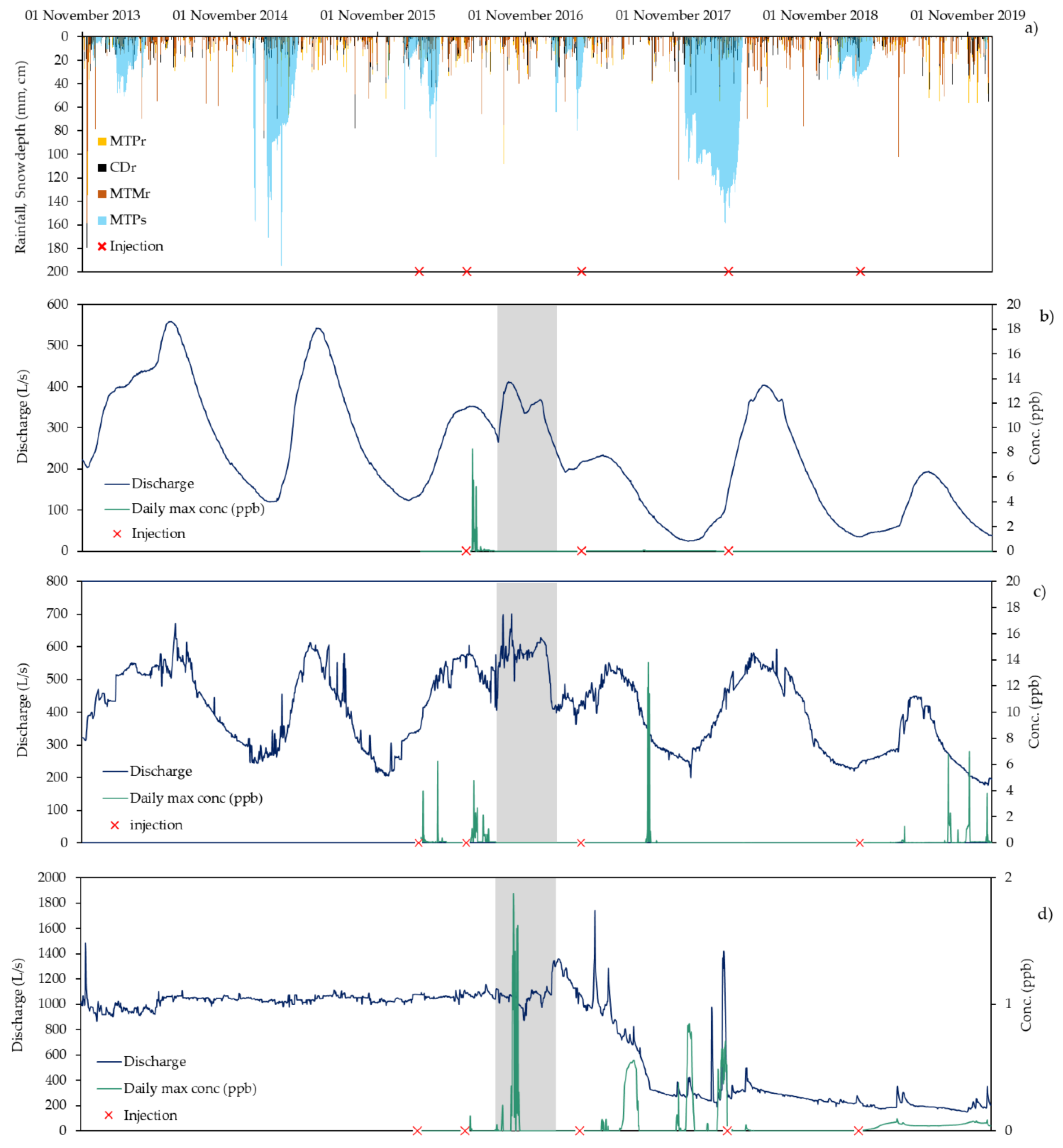
3.1. Data Description and Basic Statistics

Table 3 and Figure 2 show the basic statistics of all the time-series considered in this research. To discern whether significant changes caused by the series of strong seismic events, basic statistics have been calculated within three parts of the whole period of time: Pre-seismic (i.e., before the seismic events), Co-seismic (i.e., during the seismic events, when the main shocks took place), and Post-seismic (i.e., after the seismic events).
The inflow time-series (i.e., rainfall and snow cover thickness) do not show significant modifications among the three selected periods. Rainfall time-series (i.e., MTPr, CDr, and MTMr) are characterised by the typical random behaviour, as suggested by their non-Gaussian statistical distribution (strongly asymmetric, with minimum, 25th percentile, and median values equal to 0). November is the annual rainiest month, characterised by several intense rainfall events (>100 mm), while the driest season is generally in summer. As concerns the snow cover thickness in the recharge area (MTPs), it is characterised by a seasonal variability with a maximum value of 195 cm, reached the pre-seismic period (Figure 2). The snowfall events usually start in late November and the snow coverage remains in the highest portion of the Sibillini Massif until March-April.
Regarding the spring discharges, PES and CD are characterised by a similar behaviour with marked seasonal variability, as demonstrated by the differences between minimum and maximum values and between 25th and 75th percentiles. For FOC spring, the seasonal fluctuations are from very limited (i.e., in the order of tens of litres) to nihil. The actual nature of the baseflow feeding the different springs accounts for this evidence: PES and CD springs behaviour depends mostly on the seasonal recharge, while groundwater discharging in FOC is related to a longer and deeper circulation.
During the Co-seismic period, all the analysed springs showed an unusual increase of the discharge value, not linked to clear meteo-climatic changes [12]. For all the springs, spotless changes in their behaviour between the Pre- and Post-seismic period have been detected. The spring discharges decrease considerably after the Co-seismic period. This is clearly indicated by all the statistics shown in Table 3 (i.e., mean, minimum, 25th percentile, median, 75th percentile, and maximum values). However, to remove the possible influence of yearly variation in inflow volumes, the minimum value can be taken into account to point out the long-term decrease in spring discharges. As a result, PES, CD, and FOC springs suffered a net discharge loss (i.e., the difference between the minimum discharge values related to the Pre- and Post-seismic periods) of about 100, 5, and 720 L/s, respectively. The regional groundwater flow modifications, already highlighted in the literature [28,29], can account for these discharge losses. Furthermore, especially for FOC, the random discharge peaks are more frequent and characterised by a larger amplitude: from few litres during the Pre-seismic period to hundreds or thousands of litres after the Co-seismic one.

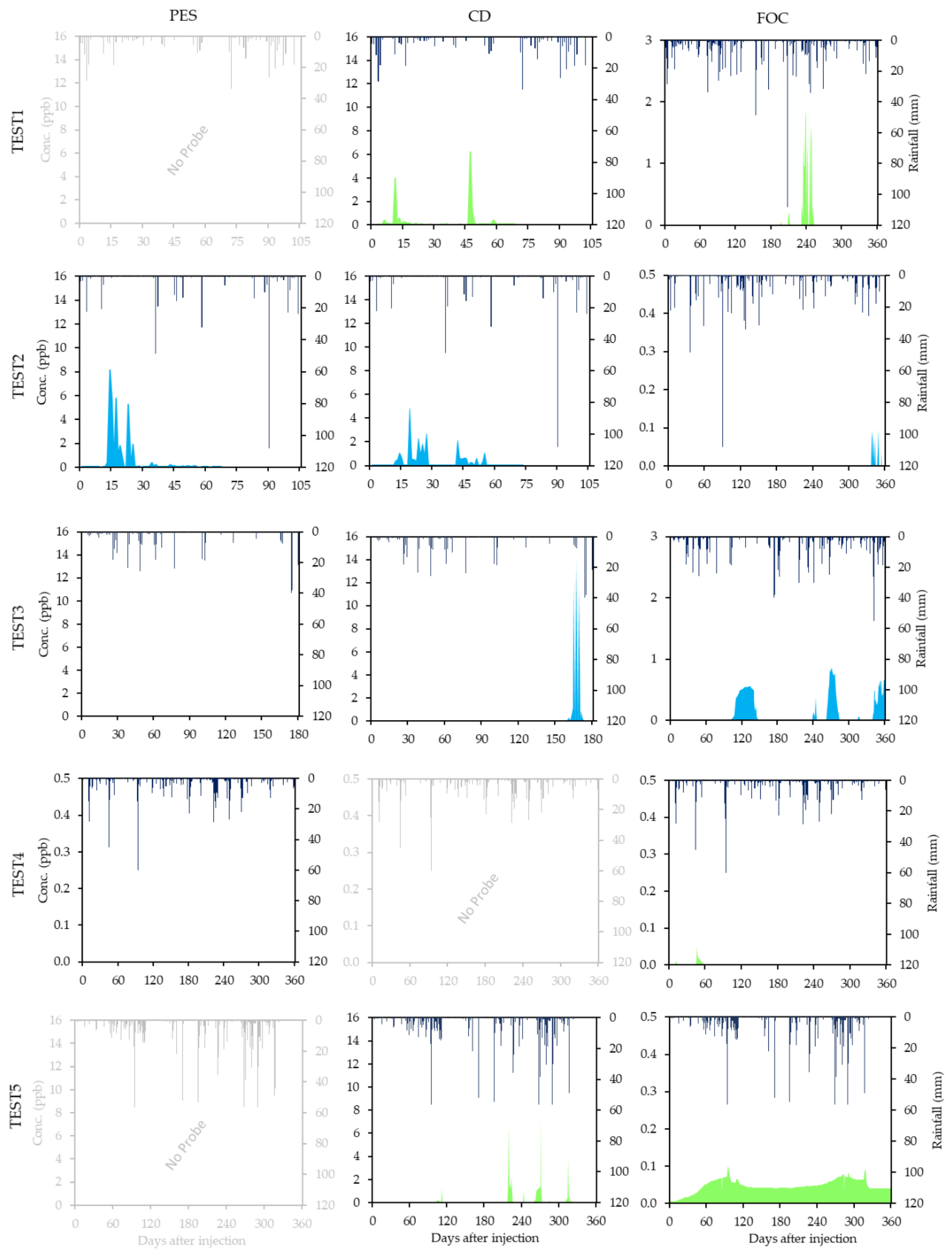
3.2. Tracer Tests Analysis

As concerns PES, only during TEST2 conducted before the series of strong seismic events on 9 June 2016, by Nanni et al. [29], the tracer arrives in the spring. The Tinopal CBS-X was recorded by the fluorimetric probe after 13 days from the injection with subsequent peaks at 18, 20, 24, and 26 days, suggesting a velocity range of tracer movement between 165–561 m/day (Table 4). During TEST3 and TEST4 conducted on 20 March 2017, and on 20 March 2018, respectively, the tracer did not arrive in PES. In all the other tests, there was no fluorimetric probe installed in the spring.
In CD, TEST1 and TEST2 show similar behaviour: the tracer arrives at the spring in about one week after the injection, showing the main peak after 12 days for TEST1 and 20 days for TEST2, respectively. Successive peaks are located between 40 and 60 days after the injection. TEST3, conducted after the main seismic events, is characterised by a lower velocity of tracer movement with respect to the others and the tracer arrives in CD between 161 and 170 days after the injection (Table 4), with the highest tracer concentration of about 14 ppb. The tracer arrivals are located in the depletion phase of the spring discharge. In TEST5, the main tracer arrivals are located in the depletion phase of the spring discharge as well. The first tracer arrival (i.e., 112 days after the injection) could be an early arrival of tracer in the spring; however, due to its low concentration, the possibility of being connected to the Fluorescein injection during TEST4 cannot be excluded. Moreover, the fluorimetric probe was not located in CD spring during the TEST4 and therefore the first peaks of tracer were not recorded. The major peaks of TEST5 are located after 217, 272, 315 days from the injection, suggesting even in this case a lower velocity of tracer for the test performed in the Pre-seismic period. A major role in the tracer velocity reduction toward the springs located in the south-eastern portion of the aquifer can be played by the blocking of karst conduits either for internal collapse or fault movement, that produced a local decrease of the hydraulic conductivity. However, since the Post-seismic period is characterised by a generalised drop of the water table, the possibility that the tracer remained stuck more easily and more often in karst conduits and fractures within a widened unsaturated zone cannot be excluded, at least in combination with the previous process.
Regarding FOC, TEST1 and TEST2 are characterised by similar behaviour in the tracer movement. The long-lasting arrivals after about 250 days and one year from the injections suggest a low velocity of tracer transit time (Table 4). Even the TEST3 is characterised by a long-lasting tracer arrival, but the peaks are located during the strong increase phases of the spring discharge (Figure 2). TEST4 and TEST5 show similar behaviour with respect to the peaks. In TEST4, the tracer was detected just after 45 days from the injection, during a strong increase of the spring discharge which passes from 312 L/s to 498 L/s in about 4 days (Figure 2). In the last test (TEST5), a small amount of tracer (>detection limit) was recorded during the whole test; however, the main peaks are located during the strong increases of the spring discharge, like TEST4.
Figure 3 illustrates the daily tracer maximum concentration and the daily rainfall recorded at MTPr station for each tracer test and spring. This representation method provides a valuable innovative alternative to highlight the correlation between tracer arrivals and the rainfall events. Interestingly, this correlation showed a delay between rainfall and tracer arrivals. The delay is interpreted as the travel time of the tracer between the recharge area and the springs. This time comprises both the infiltration in the unsaturated zone and the tracer movement in the saturated portion of the aquifers [52]. These graphs provide also information from two different points of view: the first regards the differences in the delay between injection, rainfall events, and tracer arrivals in the springs before (TEST1), during (TEST2), and after the series of strong seismic events (i.e., TEST3, TEST4, and TEST5); the second one, instead, highlights hydrogeological relationships between the different examined springs. Before the main seismic events, we notice a generally constant delay time in the arrival of the tracer after rainfall for PES and CD springs of about 10 and 8 days, respectively.
For PES spring, this aspect is documented by the peak located at about 10 days after the rainfall event, which is occurred after 3 days from the injection (TEST2). A subsequent peak is also visible at 23 days and it is likely correlated to the second intense rainfall event (>20 mm), recorded after 10 days from the injection. Regarding CD spring, there is a strong similarity in tracer arrivals between TEST1 and TEST2, but in this case, the delay time between rainfall events and tracer arrivals is slightly reduced to 8–9 days. After the rainfall events occurred 3, 10, and 36 days from the injection (TEST2), the tracer arrived at 12, 19, and 44 days after the injection. This last evidence is clearly visible in TEST2, even though confirmed by TEST1. After the seismic events, the tracer did not arrive in PES at all regardless of the presence of rainfall, while in CD spring a specific rainfall event seems to be not related to the tracer arrivals during TEST3. Analysing TEST5, a lag of 44–48 days is systematically recognised between intense rainfall events (>50 mm) and the tracer arrivals.
A completely different behaviour has been observed in FOC spring. Before and during the Co-seismic period, a specific rainfall event seems to be not related to the tracer arrivals. In this case, the relation is much more appreciable after the seismic period especially in TEST4 and TEST5, where the tracer arrives at the springs 12 days after the main rainfall events. It was also noticed that during the TEST5 a low amount of Fluorescein was recorded during the entire monitoring period. This aspect could be linked to the decrease of spring discharge (Table 3 and Figure 2), following the series of strong seismic events that occurred in this area [27]. This reduction of water volume flowing toward FOC, attributable to the change in baseflow directions, caused a limitation of dilution and allowed a larger concentration of tracer to be detected by the fluorimetric probe.

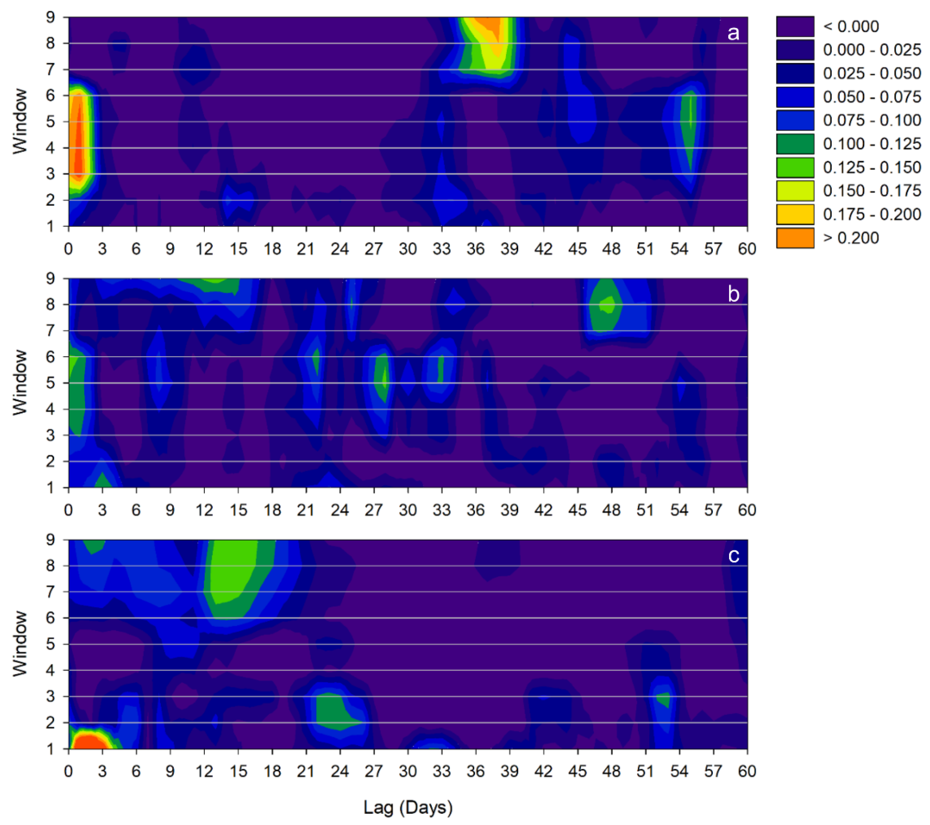
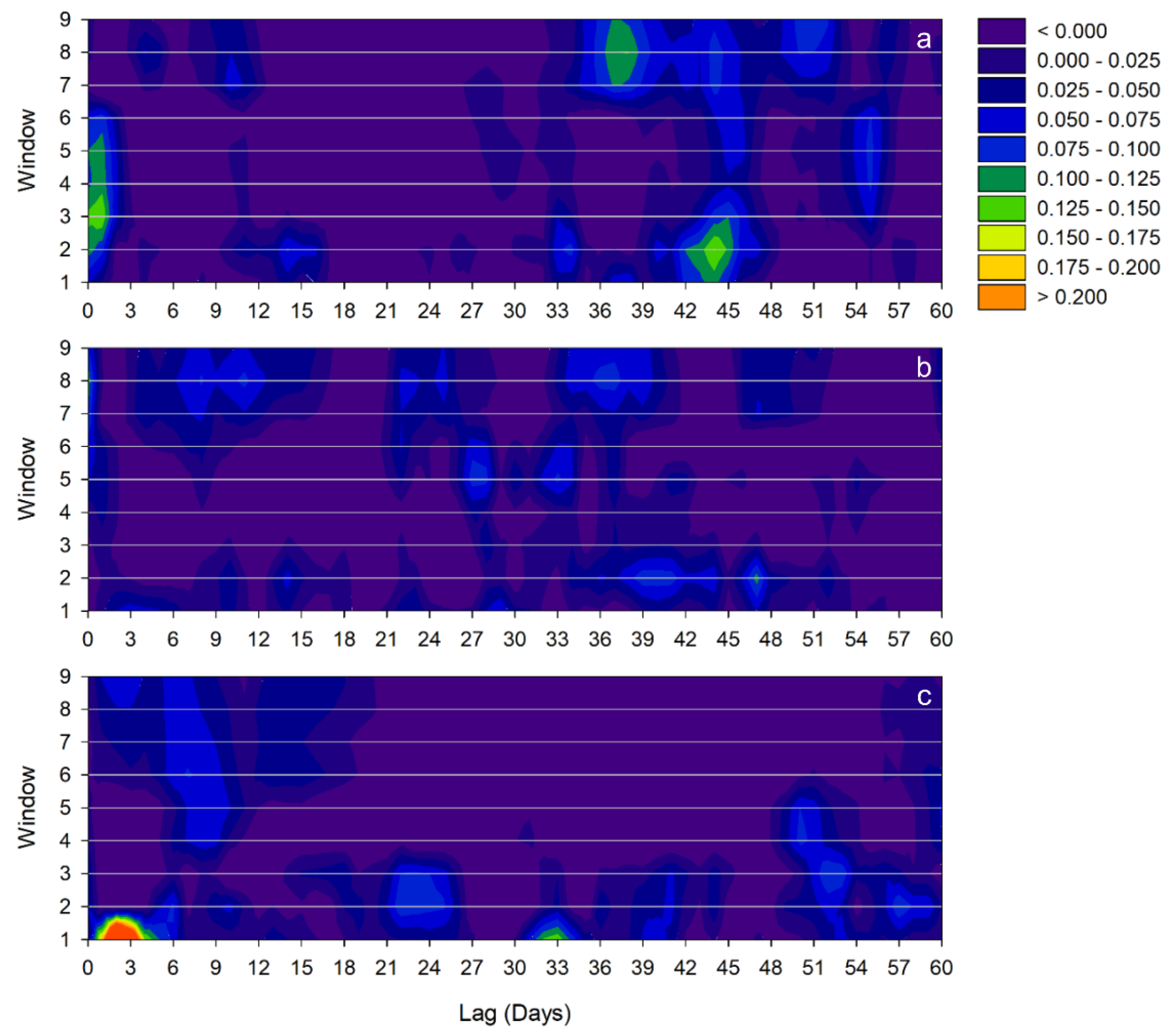
3.3. Seismically Induced Mid- and Long-Term Changes to Inflow-Outflow Relationships

In Figure 4 and Figure 5, the SWCCF results related to the Pian Grande recharge system are shown, whose time windows and corresponding seismic periods (i.e., the Pre-seismic, Co-seismic, and Post-seismic ones) are listed in Table 5. To avoid misinterpretation (e.g., false response times) of rainfall/residual spring discharge relationships for the main recharge area, the SWCCF analysis has been performed also considering the rain gauges located downstream (Figure 6), located near each spring. This has allowed a visual filtration of results shown in (Figure 5). Furthermore, it is important to highlight that all the discharge responses to the considered inflows represent the piezometric perturbations, due to the recharge arrival in the saturated zone (i.e., pressure transfer); thus, these do not necessarily include the recharge water transport through the saturated zone.
As already seen for other wide karst aquifer springs recharged mainly from snowmelt infiltration, PES and CD show a strong response to snowmelt inflow, which is represented by the high correlation values (Figure 4). However, this clear response has been pointed out mainly for the Pre- (i.e., windows 1 and 2) and Post-seismic (i.e., window 8 and 9) periods; even though it is evident also in the first and last windows of the Co-seismic period that can be considered as transition periods. In windows that fall in the central part of the Co-seismic period, the PES and CD raw spring discharges seem to totally decorrelate from snowmelt recharge, because of the transient and generalized sharp hydraulic head increase (Figure 2) related to the pore pressure propagation following strong seismic events [11,26,43]. In this case, the seasonal recharge effect on the piezometric fluctuation seems to be completely hidden by the seismically induced pore pressure propagation perturbation one. During the post-seismic period, higher correlation coefficients (i.e., CCF range is 0.4–0.6 before and 0.7–0.9 after the seismic sequence) between the PES and CD raw spring discharges and the snow cover thickness suggest a stronger influence of the seasonal recharge on these spring behaviours. Furthermore, response times increase both for PES (i.e., from about 110 to about 130 days) and CD (i.e., from about 100 to about 130 days). Taking into account that time-series of PES and CD springs (Figure 2b,c) show a clear decrease in the outflow amount, these larger response times can be attributed to local hydraulic conductivity decreases and/or a post-seismic piezometric level drop in the recharge area, that makes unsaturated a larger portion of the previously saturated zone and indeed increases the travel times of recharge water. On the other hand, FOC spring shows a very limited influence of the seasonal snowmelt inflow on the spring behaviour. In windows 1 and 2 of SWCCF between the PES and CD raw spring discharges and the snow cover thickness, the maximum significant correlation value is in the range 0.3–0.4, with a time lag of about 160 days. During the Co- and Post-seismic periods, the FOC discharge pattern seems no longer influenced by the seasonal snowmelt inflow, except for a slightly significant response with an unclear lag ranging between 60 and 90 days.
These mid- and long-term changes in the relationship between FOC discharge and snow cover thickness can be explained by a combination of (i) pore pressure propagation due to the seismic perturbation, that causes a general piezometric uprising, and (ii) non-homogeneous hydraulic conductivity variation within the of the aquifer, that has been proven to change hydrodynamics at different scales. In this area, the hydraulic conductivity increase is due to the bulk fracture cleaning triggered by the pore pressure propagation [9,11], to the formation of new co-seismic ruptures along with the Mt. Vettore-Mt. Bove fault system [53,54,55,56], and likely to the blocking of karst conduits for internal collapse and/or fault movement.
Comparing (Figure 5 and Figure 6), it appears clear that the quickest responses of residual discharge to rainfall inflow are attributable to the infiltration in the Pian Grande recharge area (MPTr). This evidence is demonstrated by the high-elevation rainfall/residual spring discharge SWCCFs, that show correlation values higher than the low-elevation rainfall/residual spring discharges’ ones.
As clearly represented in (Figure 5), all of the springs show highly different response patterns to the rainfall inflow. Before the seismic events, residual PES time-series (resPES) shows two slightly significant response peaks at about 15 and 33 days, respectively. During the Co-seismic period, a strong quick response has been (i.e., lag ~ 1–2 days, with a correlation value >0.200). At the end of the considered period (i.e., the Post-seismic), only a clear 38-day response time (i.e., correlation value > 0.200) has been pointed out detected by the rainfall/residual spring discharge SWCCF. From a hydrodynamic point of view, changes in the MTPr/resPES relationship over the considered period are related to variations in the overall piezometric level, that have affected the recharge modes.
The sharp hydraulic head increase, due to the pore pressure propagation in the Co-seismic period, has likely caused the saturation of previously unsaturated karst conduits; hence, intense rainfall events reach the water table by karst circulation and not through combined karst and diffuse fracture matrix flow paths. During the Post-seismic period, the 33-day response time raises to 38 days, due to the water table drop that likely increases the portion of unsaturated flow path toward the saturated in the diffuse fracture matrix.
The SWCCF between MTPr and the residual CD time-series (resCD) pointed out a 3-day and a 24-day significant positive response time, during the Pre-seismic period. Throughout the Co-seismic period, a very quick (i.e., 1 day) and multiple long-period (i.e., 21, 28, and 33 days) response times have been detected by the sliding window analysis. Finally, during the Post-seismic period, the response times are at 12 and 45 days. As for PES, the rise of the water table, caused by the pore pressure propagation during the Co-seismic period, has shortened the unsaturated path in the matrix of fractures, in favour of the karst one, and activated new long and/or slow paths. The following decrease of the water table has provoked a generalized increase of the response times and the deactivation of unsaturated paths, temporarily activated during the Co-seismic period. As the 45-day response time does not correspond to any of the Pre-seismic peaks, the formation of a new permanent unsaturated flow path, caused by the Mt. Vettore-Mt. Bove fault system activation, cannot be excluded.
Finally, the results related to MTPr/residual FOC spring (resFOC) sliding window time-series analysis (Figure 5) show an evident 2-day response time both in the Pre- and Post-seismic period, that disappears in the Co-seismic windows (i.e., 3–7). Furthermore, a more retarded significant peak has been detected over the considered time period. This has a lag of 24 days in the pre-seismic windows (i.e., 1 and 2), of 10 days in the central window of the Co-seismic period (i.e., 5), and 15 days in the last four windows (i.e., 6, 7, 8, and 9). The quickest response time disappears probably because it is related to an unsaturated karst flow path, that actually brings a smaller amount of recharge water toward the saturated zone; thus, the generalized pore pressure propagation throughout the Sibillini aquifer following the repeated seismic solicitations can have masked the response of resFOC. Regarding the more retarded peak, although the pore pressure propagation can account for the decrease of the response time during the Co-seismic period, its lag during the Post-seismic one has been reduced to 15 days likely because Co-seismic deformation could have created new fractures that have increased the hydraulic conductivity.

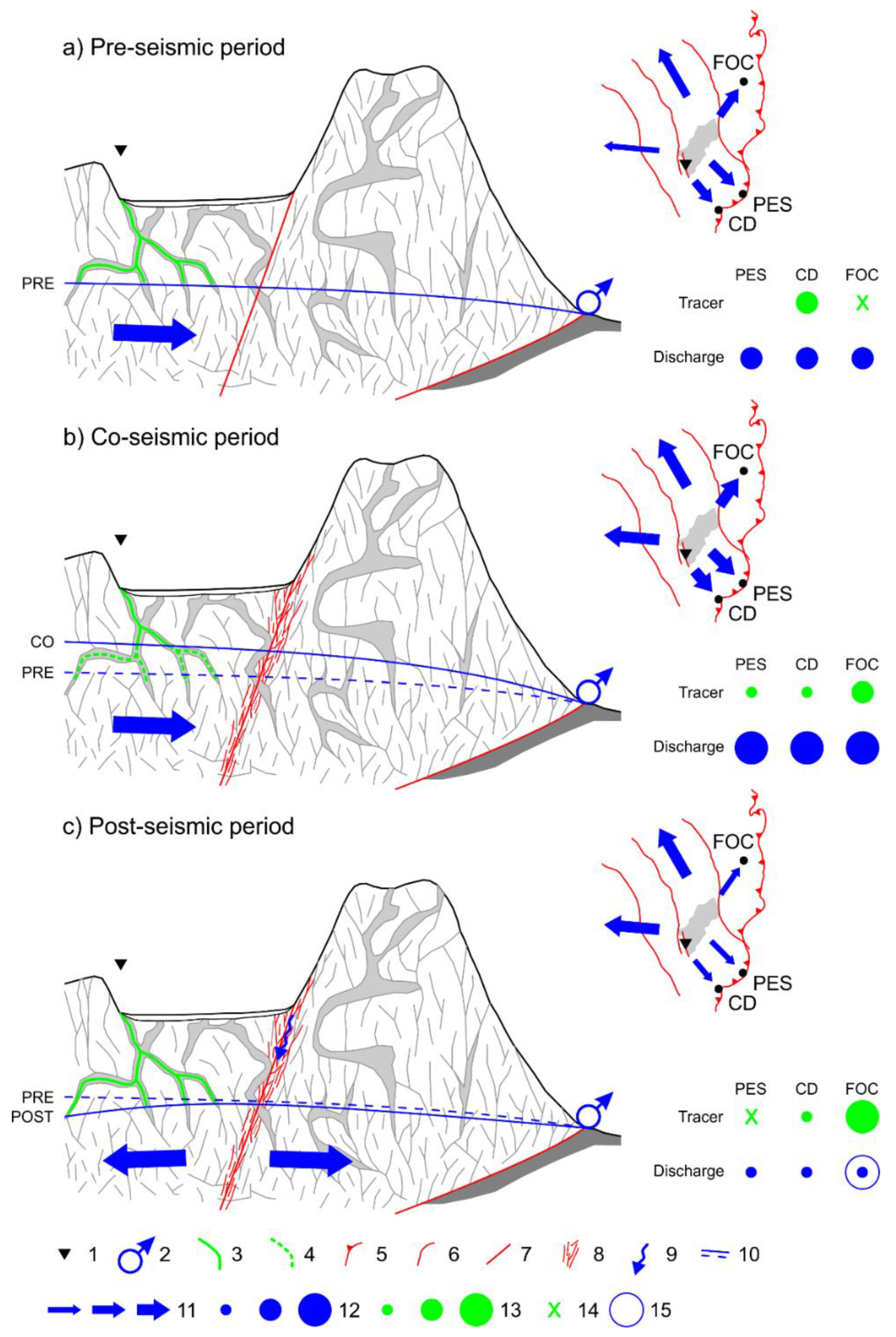
3.4. Conceptual Model

The combined approach between tracer tests and time-series analysis has allowed setting up a detailed conceptual model of the area before, during, and after the series of strong seismic events occurred in the 2016–2017 period (Figure 7). As a matter of fact, hydrodynamic changes both at a local scale and regional scale can be pointed out for the eastern side of Sibillini aquifer.
During the Pre-seismic period (Figure 7a), the baseflow fed all the springs located on the eastern side of the aquifer; however, the SWCCF between the snow cover thickness and the raw spring discharge pointed out that the snowmelt recharge influenced considerably only the PES and CD discharge, while the FOC regime did not show any seasonal variation. The tracer injected in the Mèrgani sinkhole to simulate the recharge process arrived in the south-eastern sector (i.e., CD spring) in about 10–20 days, while reaches FOC in more than 200 days. Intense rainfall events infiltrating during the Pre-seismic period affected the discharge patterns by reaching the saturated zone with travel times of few days for CD and FOC and tens of days for all the spring on the eastern portion of Sibillini aquifer. Therefore, these rainfall events mobilised the tracer stack in the unsaturated zone, bringing it to the spring with an additional delay of few days.
This complex but defined framework changed considerably during the Co-seismic period (Figure 7b) because subsequent strong seismic events caused a pore pressure propagation throughout the entire aquifer. This phenomenon accounts for the complete disappearance of the seasonal response in the SWCCF between the snow cover thickness and all the raw discharge time-series. Besides, another result of the pore pressure propagation was the generalised transient increase of the hydraulic head, which can explain the quicker response of the discharge of all the springs to intense rainfall events. The water table rise provoked the saturation of a shallower portion of the aquifer that is expected to have porosity more attributable to karst features than to fracture ones. For the same reason, other additional flow paths previously unsaturated were activated, as highlighted especially in CD by the SWCCF between rainfall and residual spring discharge time-series. Although changes in the relationships between the rainfall recharge and spring discharge were observed from a hydrodynamic standpoint, no significant variations were detected in the tracer travel times after intense rainfall events.
In the Post-seismic period (Figure 7c), the irreversible effects of the series of strong seismic events affected the Sibillini aquifer hydrodynamics. In fact, the Mt. Vettore-Mt. Bove fault system activation, together with multiple ground shakings, caused consistent variations in the hydraulic conductivity distribution throughout the aquifer, either by increasing or reducing its value. The fault system activation produced new co-seismic ruptures and fractures [54,55,56], while the ground shaking caused the already existing void clean up [9,11]. This heterogeneous hydraulic conductivity increase within the aquifer provoked a general lowering of the piezometric level, especially in the recharge area, and a shift on the groundwater divide with a subsequent hydraulic gradient variation, as already noticed in literature [26,28,29]. As a result, the regional groundwater flow direction changed considerably, becoming north-west. This variation in the regional groundwater flow accounts for the clear discharge decrease in all the considered springs. Besides, both snowmelt (Figure 4) and rainfall (Figure 5) travel times increased, especially in PES and CD, as pointed out by the SWCCF results.
Comparing the tracer velocity variations between the Pre- and Post-seismic periods (Table 4), additional insights about irreversible changes due to the 2016–2017 period on the distribution of hydraulic conductivity can be obtained. In detail, FOC shows a higher tracer velocity, that is attributable to the hydraulic conductivity increase due to the co-seismic ruptures. Besides, this new fracture network created a more permeable zone in the area between the Mèrgani sinkhole and FOC favouring a more rapid infiltration of intense rainfall events, that arrived in the spring in 2 days (Figure 5). In FOC, the simultaneous arrivals of the tracer and the abrupt and consistent discharge increase confirmed the crucial role of the co-seismic ruptures in changing this spring hydrodynamics. Contrariwise, a decrease in the overall tracer velocity has been observed in PES and CD. Although it could be ascribable to the water table drop and the subsequent widening of the unsaturated zone increasing the probability for the tracer to remain stack in karst conduits and fractures, a local decrease of the hydraulic conductivity caused by the blocking of karst conduits for internal collapse and/or fault movement could have played a major role in this extension of the travel times toward the south-eastern portion of the Sibillini aquifer.

4. Conclusions

In this research, the main objective was to get a deeper insight into the effects that a series of strong seismic events can have on the hydrodynamic of a limestone aquifer and to the discharge regime of its springs, both at mid- and long-term. The availability of rainfall, snow cover thickness, and discharge daily time-series, collected over a 6-year time interval that comprises the 2016–2017 seismic period, and high-quality tracer tests, performed at different times along the same period, has enabled to define a detailed framework of reversible and irreversible modifications to the aquifer features and to the recharge system that affected the Sibillini massif’s springs, located on its eastern side. To this purpose, these valuable datasets have been analysed through a combined approach, that takes into account periodic tracer tests and the Sliding-Window Cross-Correlation Function.
The combination of ground shaking and fault activation caused reversible and irreversible mid- and long-term variations of the hydraulic conductivity (i.e., both increases and decreases) within the Sibillini aquifer that changed its recharge system at different scales and the spring discharge regime. In detail, the void cleaning induced by the pore pressure propagation throughout the aquifer and the creation of co-seismic ruptures caused a modification of the groundwater flow, a general decrease of the water table as well as a shift of the groundwater divide eastward, and improved the rainfall infiltration toward FOC spring. On the other hand, the blocking of karst conduits for internal collapse and/or fault movement accounted for the local decrease of the hydraulic conductivity that slowed down the groundwater flow toward both PES and CD springs.
As a result, this research has tried to compare two techniques aimed at understanding underground hydrodynamics, which usually provides results at different time scales: periodic tracer tests and transient time-series analysis. In the first case, single and localized inflow events and their spatio-temporal influence on the recharge system are simulated; hence, the strong heterogeneity and anisotropy of the system, as well as the meteo-climatic features of the specific year, have a major influence on the results, although the tracer behaviour reflects the actual flow of recharge water. In the second case, the time-series analysis techniques allow identifying the inflow-outflow relationships along with large time scales and independently from the number and intensity of the recharge events. Although this is the first attempt to join time-series analysis and tracer tests and limitations can be found in both cases, the outstanding results obtained by the proposed combined approach gives the chance to statistically explain the tracer path within the aquifer, especially when the tracer gets stuck in the highly heterogeneous unsaturated zone and are mobilized by consecutive recharge events. Considering the promising results obtained through this approach, it can be certainly applied in similar geological contexts worldwide.

Author Contributions

Conceptualization, D.F., D.D.C., A.T., and S.R.; methodology, D.F. and D.D.C.; data analysis, D.F., and D.D.C., D.V.; writing—original draft preparation, D.F. and D.D.C.; writing—review and editing, D.D.C., D.F., S.R., and A.T.; visualization, D.F., D.D.C., and S.R.; project administration, A.T.; funding acquisition, A.T. and D.V. All authors have read and agreed to the published version of the manuscript.

Funding

This research was financed by Regione Umbria, Italy, Funds for “Interventi di emergenza previsti dall’Ordinanza del Capo del Dipartimento di Protezione Civile del 26 agosto 2016, n. 388” and by C.I.I.P Servizio idrico Integrato.

Acknowledgments

We kindly acknowledge C.I.I.P Servizio idrico Integrato for providing discharge data of the analysed springs, and the Regione Marche—Servizio Protezione Civile, Centro Funzionale Multirischi per la meteorologia, l’idrologia e la sismologia for providing meteorological data. Many thanks to Stefano Palpacelli and Mirco Marcellini for the effort made to support the tracer tests field operations. We would also like to thank all the reviewers for their helpful comments, which improved the text considerably.

Conflicts of Interest

The authors declare no conflict of interest.

References

  1. Manga, M.; Wang, C.-Y. Earthquake Hydrology. In Treatise on Geophysics; Elsevier BV: Oxford, UK, 2015; Volume 4, pp. 305–328. [Google Scholar]
  2. Charmoille, A.; Fabbri, O.; Mudry, J.; Guglielmi, Y.; Bertrand, C. Post-seismic permeability change in a shallow fractured aquifer following a ML5.1 earthquake (Fourbanne karst aquifer, Jura outermost thrust unit, eastern France). Geophys. Res. Lett. 2005, 32, 32. [Google Scholar] [CrossRef]
  3. Esposito, E.; Pece, R.; Porfido, S.; Tranfaglia, G. Ground effects and hydrological changes in the Southern Apennines (Italy) in response to the 23 July 1930 earthquake (MS=6.7). Nat. Hazards Earth Syst. Sci. 2009, 9, 539–550. [Google Scholar] [CrossRef] [Green Version]
  4. De Luca, G.; Di Carlo, G.; Tallini, M. A record of changes in the Gran Sasso groundwater before, during and after the 2016 Amatrice earthquake, central Italy. Sci. Rep. 2018, 8, 15982. [Google Scholar] [CrossRef] [PubMed]
  5. De Luca, G.; Di Carlo, G.; Tallini, M. Signals from groundwater in Gran Sasso underground laboratory during Amatrice earthquake of August 24th, 2016. Ann. Geophys. 2016, 59. [Google Scholar] [CrossRef]
  6. Lai, W.-C.; Koizumi, N.; Matsumoto, N.; Kitagawa, Y.; Lin, C.-W.; Shieh, C.-L.; Lee, Y.-P. Effects of seismic ground motion and geological setting on the coseismic groundwater level changes caused by the 1999 Chi-Chi earthquake, Taiwan. Earth Planets Space 2004, 56, 873–880. [Google Scholar] [CrossRef] [Green Version]
  7. Manga, M.; Rowland, J.C. Response of Alum Rock springs to the October 30, 2007 Alum Rock earthquake and implications for the origin of increased discharge after earthquakes. Geofluids 2009, 9, 237–250. [Google Scholar] [CrossRef]
  8. Montgomery, D.R. Streamflow and Water Well Responses to Earthquakes. Science 2003, 300, 2047–2049. [Google Scholar] [CrossRef] [Green Version]
  9. Adinolfi Falcone, R.; Carucci, V.; Falgiani, A.; Manetta, M.; Parisse, B.; Petitta, M.; Rusi, S.; Spizzico, M.; Tallini, M. Changes on groundwater flow and hydrochemistry of the Gran Sasso carbonate aquifer after 2009 L’Aquila earthquake. Ital. J. Geosci. 2012, 131, 459–474. [Google Scholar] [CrossRef]
  10. Koizumi, N.; Minote, S.; Tanaka, T.; Mori, A.; Ajiki, T.; Sato, T.; Takahashi, H.A.; Matsumoto, N. Hydrological changes after the 2016 Kumamoto earthquake, Japan. Earth Planets Space 2019, 71, 1–10. [Google Scholar] [CrossRef]
  11. Amoruso, A.; Crescentini, L.; Petitta, M.; Rusi, S.; Tallini, M. Impact of the 6 April 2009 L’Aquila earthquake on groundwater flow in the Gran Sasso carbonate aquifer, Central Italy. Hydrol. Process. 2010, 25, 1754–1764. [Google Scholar] [CrossRef]
  12. Valigi, D.; Fronzi, D.; Cambi, C.; Beddini, G.; Cardellini, C.; Checcucci, R.; Mastrorillo, L.; Mirabella, F.; Tazioli, A. Earthquake-Induced Spring Discharge Modifications: The Pescara di Arquata Spring Reaction to the August–October 2016 Central Italy Earthquakes. Water 2020, 12, 767. [Google Scholar] [CrossRef] [Green Version]
  13. Dar, F.A.; Perrin, J.; Ahmed, S.; Narayana, A.C. Review: Carbonate aquifers and future perspectives of karst hydrogeology in India. Hydrogeol. J. 2014, 22, 1493–1506. [Google Scholar] [CrossRef]
  14. Bakalowicz, M. Karst groundwater: A challenge for new resources. Hydrogeol. J. 2005, 13, 148–160. [Google Scholar] [CrossRef]
  15. Manga, M.; ABeresnev, I.; Brodsky, E.E.; ElKhoury, J.E.; Elsworth, D.; Ingebritsen, S.E.; Mays, D.C.; Wang, C.-Y. Changes in permeability caused by transient stresses: Field observations, experiments, and mechanisms. Rev. Geophys. 2012, 50, 50. [Google Scholar] [CrossRef]
  16. Fiorillo, F.; Doglioni, A. The relation between karst spring discharge and rainfall by cross-correlation analysis (Campania, southern Italy). Hydrogeol. J. 2010, 18, 1881–1895. [Google Scholar] [CrossRef]
  17. Lambrakis, N.; Andreou, A.S.; Polydoropoulos, P.; Georgopoulos, E.; Bountis, T. Nonlinear analysis and forecasting of a brackish Karstic spring. Water Resour. Res. 2000, 36, 875–884. [Google Scholar] [CrossRef]
  18. Larocque, M.; Mangin, A.; Razack, M.; Banton, O. Contribution of correlation and spectral analyses to the regional study of a large karst aquifer (Charente, France). J. Hydrol. 1998, 205, 217–231. [Google Scholar] [CrossRef]
  19. Mathevet, T.; Lepiller, M.L.; Mangin, A. Application of time-series analyses to the hydrological functioning of an Alpine karstic system: The case of Bange-L’Eau-Morte. Hydrol. Earth Syst. Sci. 2004, 8, 1051–1064. [Google Scholar] [CrossRef]
  20. Aquilanti, L.; Clementi, F.; Landolfo, S.; Nanni, T.; Palpacelli, S.; Tazioli, A. A DNA tracer used in column tests for hydrogeology applications. Environ. Earth Sci. 2013, 70, 3143–3154. [Google Scholar] [CrossRef]
  21. Tazioli, A.; Aquilanti, L.; Clementi, F.; Marcellini, M.; Nanni, T.; Palpacelli, S.; Vivalda, P.M. Hydraulic contacts identification in the aquifers of limestone ridges: Tracer tests in the Montelago pilot area (Central Apennines). Acque Sotter. Ital. J. Groundw. 2016, 5. [Google Scholar] [CrossRef] [Green Version]
  22. Mudarra, M.; Hartmann, A.; Andreo, B. Combining Experimental Methods and Modeling to Quantify the Complex Recharge Behavior of Karst Aquifers. Water Resour. Res. 2019, 55, 1384–1404. [Google Scholar] [CrossRef]
  23. Chiaraluce, L.; Di Stefano, R.; Tinti, E.; Scognamiglio, L.; Michele, M.; Casarotti, E.; Cattaneo, M.; De Gori, P.; Chiarabba, C.; Monachesi, G.; et al. The 2016 Central Italy Seismic Sequence: A First Look at the Mainshocks, Aftershocks, and Source Models. Seismol. Res. Lett. 2017, 88, 757–771. [Google Scholar] [CrossRef]
  24. Di Matteo, L.; Dragoni, W.; Azzaro, S.; Pauselli, C.; Porreca, M.; Bellina, G.; Cardaci, W.; Lucio, D.M.; Dragoni, W.; Salvatore, A.; et al. Effects of earthquakes on the discharge of groundwater systems: The case of the 2016 seismic sequence in the Central Apennines, Italy. J. Hydrol. 2020, 583, 124509. [Google Scholar] [CrossRef]
  25. Fronzi, D.; Banzato, F.; Caliro, S.; Cambi, C.; Cardellini, C.; Checcucci, R.; Mastrorillo, L.; Mirabella, F.; Petitta, M.; Valigi, D.; et al. Preliminary results on the response of some springs of the Sibillini Mountains area to the 2016-2017 seismic sequence. Acque Sotter. Ital. J. Groundw. 2020. [Google Scholar] [CrossRef] [Green Version]
  26. Petitta, M.; Mastrorillo, L.; Preziosi, E.; Banzato, F.; Barberio, M.D.; Billi, A.; Cambi, C.; De Luca, G.; Di Carlo, G.; Di Curzio, D.; et al. Water-table and discharge changes associated with the 2016–2017 seismic sequence in central Italy: Hydrogeological data and a conceptual model for fractured carbonate aquifers. Hydrogeol. J. 2018, 26, 1009–1026. [Google Scholar] [CrossRef] [Green Version]
  27. Valigi, D.; Mastrorillo, L.; Cardellini, C.; Checcucci, R.; Di Matteo, L.; Frondini, F.; Mirabella, F.; Viaroli, S.; Vispi, I. Springs discharge variations induced by strong earthquakes: The Mw 6.5 Norcia event (Italy, October 30th 2016). Rendiconti Online Soc. Geol. Ital. 2019, 47, 141–146. [Google Scholar] [CrossRef]
  28. Mastrorillo, L.; Saroli, M.; Viaroli, S.; Banzato, F.; Valigi, D.; Petitta, M. Sustained post-seismic effects on groundwater flow in fractured carbonate aquifers in Central Italy. Hydrol. Process. 2019, 34, 1167–1181. [Google Scholar] [CrossRef] [Green Version]
  29. Nanni, T.; Vivalda, P.M.; Palpacelli, S.; Marcellini, M.; Tazioli, A. Groundwater circulation and earthquake-related changes in hydrogeological karst environments: A case study of the Sibillini Mountains (central Italy) involving artificial tracers. Hydrogeol. J. 2020, 1–20. [Google Scholar] [CrossRef]
  30. Banzato, F.; Mastrorillo, L.; Nanni, T.; Palpacelli, S.; Petitta, M.; Vivalda, P.M. L’acquifero carbonatico fratturato delle Sorgenti del Fiume Aso (Parco Nazionale dei Monti Sibillini): Valutazioni sulla risorsa rinnovabile e sull’area di alimentazione. In Proceedings of the “La ricerca carsologica in Italia” Laboratorio Carsologico Sotterraneo di Bossea, Frabosa Soprana, Italy, 22–23 June 2013. [Google Scholar]
  31. Nanni, T. Caratteri idrogeologici delle Marche. In L’ambiente Fisico delle Marche; S.E.C.L.A. s.r.l.: Florence, Italy, 1991. [Google Scholar]
  32. Mastrorillo, L.; Baldoni, T.; Banzato, F.; Boscherini, A.; Cascone, D.; Checcucci, R.; Boni, C. Quantitative hydrogeological analysis of the carbonate domain of the Umbria Region (Central Italy). Ital. J. Eng. Geol. Environ. 2009, 1, 137–155. [Google Scholar]
  33. Aquilanti, L.; Clementi, F.; Nanni, T.; Palpacelli, S.; Tazioli, A.; Vivalda, P.M. DNA and fluorescein tracer tests to study the recharge, groundwater flowpath and hydraulic contact of aquifers in the Umbria-Marche limestone ridge (central Apennines, Italy). Environ. Earth Sci. 2016, 75, 1–17. [Google Scholar] [CrossRef]
  34. Calamita, F. Thrusts and fold-related structures in the Umbria-Marche Apennines (Central Italy). Ann. Tecto. 1990, 4, 83–117. [Google Scholar]
  35. Pierantoni, P.; Deiana, G.; Galdenzi, S. Stratigraphic and structural features of the Sibillini Mountains (Umbria-Marche Apennines, Italy). Ital. J. Geosci. 2013, 132, 497–520. [Google Scholar] [CrossRef]
  36. Lavecchia, G. II sovrascorrimento dei Monti Sibillini: Analisi cinematica e strutturale. Boll. Soc. Geol. It. 1985, 104, 161–194. [Google Scholar]
  37. Calamita, F.; Deiana, G. Evoluzione Strutturale Neogenico-Quaternaria Dell’appennino Umbro-Marchigiano. Available online: http://193.204.8.201:8080/jspui/bitstream/1336/204/1/Vol.%20Geologia%20Marche%20Capitolo%208.pdf (accessed on 2 November 2020).
  38. Dragoni, W.; Speranza, G.; Valigi, D. Impatto delle variazioni climatiche sui sistemi idrogeologici: II caso della sorgente Pescara di Arquata (Appennino umbro-marchigiano, Italia). Geol. Tec. Ambient. 2003, 3, 27–35. [Google Scholar]
  39. Boni, C. Hydrogeological study for identification, characterisation and management of groundwater resources in the Sibillini Mountains National Park (Central Italy). Ital. J. Eng. Geol. Environ. 2010, 21–39. [Google Scholar] [CrossRef]
  40. Lippi Boncambi, C. Soil observations on the Sibillini Mountains, in particular on the peaty soils of the Castelluccio di Norcia plain. Boll. Soc. Geol. It. 1950, 69, 26–37. [Google Scholar]
  41. US EPA. The Qtracer2 Program for Tracer-Breakthrough Curve Analysis for Tracer Tests in Karstic Aquifers and Other Hydrologic Systems; EPA/600/R-02/001; US Environmental Protection Agency, Office of Research and Development, National Centre for Environmental Assessment: Washington, DC, USA, 2002. Available online: https://cfpub.epa.gov/ncea/risk/recordisplay.cfm?deid=54930 (accessed on 2 November 2020).
  42. Delbart, C.; Valdes, D.; Barbecot, F.; Tognelli, A.; Richon, P.; Couchoux, L. Temporal variability of karst aquifer response time established by the sliding-windows cross-correlation method. J. Hydrol. 2014, 511, 580–588. [Google Scholar] [CrossRef]
  43. Chiaudani, A.; Di Curzio, D.; Palmucci, W.; Pasculli, A.; Polemio, M.; Rusi, S. Statistical and Fractal Approaches on Long Time-Series to Surface-Water/Groundwater Relationship Assessment: A Central Italy Alluvial Plain Case Study. Water 2017, 9, 850. [Google Scholar] [CrossRef] [Green Version]
  44. Viaroli, S.; Di Curzio, D.; Lepore, D.; Mazza, R. Multiparameter daily time-series analysis to groundwater recharge assessment in a caldera aquifer: Roccamonfina Volcano, Italy. Sci. Total Environ. 2019, 676, 501–513. [Google Scholar] [CrossRef]
  45. Nanni, T.; Rusi, S. Idrogeologia del massiccio carbonatico della Majella (Abruzzo). Boll. Soc. Geol. It. 2003, 122, 173–202. [Google Scholar]
  46. Fiorillo, F.; Petitta, M.; Preziosi, E.; Rusi, S.; Esposito, L.; Tallini, M. Long-term trend and fluctuations of karst spring discharge in a Mediterranean area (central-southern Italy). Environ. Earth Sci. 2014, 74, 153–172. [Google Scholar] [CrossRef]
  47. Rusi, S.; Di Curzio, D.; Palmucci, W.; Petaccia, R. Detection of the natural origin hydrocarbon contamination in carbonate aquifers (central Apennine, Italy). Environ. Sci. Pollut. Res. 2018, 25, 15577–15596. [Google Scholar] [CrossRef] [PubMed]
  48. Chiaudani, A.; Di Curzio, D.; Rusi, S. The snow and rainfall impact on the Verde spring behavior: A statistical approach on hydrodynamic and hydrochemical daily time-series. Sci. Total Environ. 2019, 689, 481–493. [Google Scholar] [CrossRef]
  49. Gregor, M. BFI+ 3.0 User’s Manual (21pp) 2010. Available online: https://hydrooffice.org/Files/UM%20BFI.pdf (accessed on 30 October 2020).
  50. Sloto, R.A.; Crouse, M.Y. HYSEP: A Computer Program for Streamflow Hydrograph Separation and Analysis. Water Resour. Investig. Rep. 1996, 96, 4040. [Google Scholar] [CrossRef]
  51. Seidenbecher, T. Amygdalar and Hippocampal Theta Rhythm Synchronization During Fear Memory Retrieval. Science 2003, 301, 846–850. [Google Scholar] [CrossRef] [Green Version]
  52. Mudarra, M.; Andreo, B. Relative importance of the saturated and the unsaturated zones in the hydrogeological functioning of karst aquifers: The case of Alta Cadena (Southern Spain). J. Hydrol. 2011, 397, 263–280. [Google Scholar] [CrossRef]
  53. Evans, J.P.; Forster, C.B.; Goddard, J.V. Permeability of fault-related rocks, and implications for hydraulic structure of fault zones. J. Struct. Geol. 1997, 19, 1393–1404. [Google Scholar] [CrossRef]
  54. Porreca, M.; Minelli, G.; Ercoli, M.; Brobia, A.; Mancinelli, P.; Cruciani, F.; Giorgetti, C.; Carboni, F.; Mirabella, F.; Cavinato, G.; et al. Seismic Reflection Profiles and Subsurface Geology of the Area Interested by the 2016-2017 Earthquake Sequence (Central Italy). Tectonics 2018, 37, 1116–1137. [Google Scholar] [CrossRef]
  55. Villani, F.; Pucci, S.; Civico, R.; De Martini, P.M.; Cinti, F.; Pantosti, D. Surface Faulting of the 30 October 2016 Mw 6.5 Central Italy Earthquake: Detailed Analysis of a Complex Coseismic Rupture. Tectonics 2018, 37, 3378–3410. [Google Scholar] [CrossRef]
  56. Puliti, I.; Pizzi, A.; Benedetti, L.; Di Domenica, A.; Fleury, J. Comparing Slip Distribution of an Active Fault System at Various Timescales: Insights for the Evolution of the Mt. Vettore-Mt. Bove Fault System in Central Apennines. Tectonics 2020, 39. [Google Scholar] [CrossRef]
Figure 1. Hydrogeological sketch of the study area and location of the monitoring points. 1. Thrust fault; 2. Normal fault; 3. Alluvial and lacustrine deposits (Holocene-Pliocene); 4. Clay and sands units (Miocene); 5. Calcareous Marly units (Miocene-Eocene); 6. Scaglia Calcarea (Eocene-Cretaceous); 7. Marne a Fucoidi (Lower Cretaceous); 8. Maiolica (Lower Cretaceous-Jurassic); 9. Calcareous siliceous marly units (Upper Jurassic); 10. Corniola-Calcare Massiccio (Lower Jurassic); 11. Anidriti di Burano (Triassic); 12. Rain gauges and snow thickness gauge (see Table 1); 13. Spring discharge station with fluorimetric probes; 14. Tracer injection point. 15. Hydrogeological section. All the cross-sections are modified from the literature [29,38].
Water 12 03073 g001
Figure 2. Graphs of the considered time-series: (a) Daily rainfall recorded at Mount Prata rain (MTPr), Capodacqua rain (CDr), and Montemonaco rain (MTMr) gauges and snow cover thickness data measured at Mount Prata snow (MTPs) gauge starting from November 2013 to December 2019. The red crosses represent the injection of tracer in the Mèrgani sinkhole. Daily discharge expressed in L/s and tracer maximum concentration expressed in ppb, recorded at (b) Pescara springs (PES), (c) Capodacqua (CD), and d) Foce spring (FOC), respectively, starting from November 2013 to December 2019. In those cases, the red crosses represent the presence of a fluorimetric probe in the monitoring points. The grey zone represents the most intensive seismic period (24 August 2016–18 January 2017).
Water 12 03073 g002
Figure 3. Comparison between tracer concentration expressed in ppb vs days after injection in the monitoring points and rainfall recorded at MTPr during the five analysed tests. The green area represents the Fluorescein, while the blue one the Tinopal CBS-X. When the fluorimetric probe was not installed in a specific spring during a specific test, the corresponding graph is represented in light grey, and the expression “No Probe” is added in the figure.
Water 12 03073 g003
Figure 4. Contour graphs that represent variations in the curve shape of the snow cover/ raw spring discharge CCFs, over the whole period (i.e., among the sliding windows shown in (Table 5). (a) MTPs/PES; (b) MTPs/CD; (c) MTPs/FOC. The positive correlation value corresponding to the 95% significance level (p < 0.05) is 0.06.
Water 12 03073 g004
Figure 5. Contour graphs that represent variations in the curve shape of the high-elevation rainfall/residual spring discharge CCFs, over the whole period (i.e., among the sliding windows shown in Table 5). (a) MTPr/resPES; (b) MTPr/resCD; (c) MTPr/resFOC. The positive correlation value corresponding to the 95% significance level (p < 0.05) is 0.06.
Water 12 03073 g005
Figure 6. Contour graphs that represent variations in the curve shape of the low-elevation rainfall/residual spring discharge CCFs, over the whole period (i.e., among the sliding windows shown in Table 5). (a) CDr/resPES; (b) CDr/resCD; (c) MTMr/resFOC. The positive correlation corresponding related to the 95% significance level (p < 0.05) is 0.06.
Water 12 03073 g006
Figure 7. Schematic conceptual model. On the left, hydrogeological cross-sections (not in scale); on the right, plan views of the analyzed springs and recharge area (not in scale). In legend: (1) tracer injection point (i.e., Mèrgani sinkhole); (2) spring; (3) tracer; (4) diluted tracer; (5) thrust in plan views; (6) normal fault in plan views; (7) tectonic structures in cross-section; (8) co-seismic ruptures; (9) rainfall infiltration; (10) piezometric levels; (11) Basal aquifer main groundwater flow direction (the symbol size is proportional to the quantity: low, intermediate, high); (12) spring discharge (the symbol size is proportional to the quantity: low, intermediate, high); (13) recovered tracer (the symbol size is proportional to the quantity: low, intermediate, high); (14) tracer not recovered; (15) strong discharge response to intense rainfall events.
Water 12 03073 g007
Table 1. Details of the points of the monitoring network considered in this research.
PointAbbreviationParameterInstrument
Pescara springPESDischargeWater level gauge
Capodacqua springCDDischargeWater level gauge
Foce springFOCDischargeWater level gauge
Monte Prata stationMTPs
MTPr
Snow cover thicknessSnow gauge
Montemonaco stationMTMrRainfallRain gauge
Capodacqua stationCDrRainfallRain gauge
RainfallRain gauge
Table 2. Characteristics of the tracer tests conducted in the area.
Test IDInjection DateTracerMass (kg)Mèrgani Discharge (L/s)PeriodReference
TEST112 February 2016Fluorescein21550Pre-seismic[29]
TEST29 June 2016Tinopal CBS-X2910Co-seismic[29]
TEST320 March 2017Tinopal CBS-X85136Post-seismic[29]
TEST420 March 2018Fluorescein16130This study
TEST508 February 2019Fluorescein2770This study
Table 3. Basic statistics of the considered time-series, related to the Pre-seismic, Co-seismic, and Post-seismic periods. See Table 1 for the monitoring points’ abbreviations.
Pre-Seismic Period
UnitN of DataMeanMin25thMedian75thMax
MTPscm102711.80.00.00.07.5195.0
MTPrmm10273.00.00.00.02.0135.0
CDrmm10273.50.00.00.02.8179.2
MTMrmm10273.60.00.00.03.2158.8
PESL/s1027309.9119.9192.8313.6412.6559.5
CDL/s1027430.3205.6326.8444.6529.8671.4
FOCL/s10271033.7866.91020.01043.71059.51476.4
Co-Seismic Period
UnitN of DataMeanMin25thMedian75thMax
MTPscm1482.60.00.00.00.064.0
MTPrmm1483.50.00.00.22.4108.2
CDrmm1483.00.00.00.22.664.2
MTMrmm1483.00.00.00.01.975.0
PESL/s148346.6242.4320.2357.0378.0412.3
CDL/s148568.3410.1559.2581.0602.7700.5
FOCL/s1481065.9871.31035.81064.31090.51343.4
Post-Seismic Period
UnitN of DataMeanMin25thMedian75thMax
MTPscm101617.80.00.00.014.7158.7
MTPrmm10162.60.00.00.01.660.0
CDrmm10162.90.00.00.02.083.4
MTMrmm10163.40.00.00.02.2121.6
PESL/s1016154.624.659.5143.5218.6404.0
CDL/s1016377.1199.5276.0376.6468.4593.9
FOCL/s1016422.0153.1221.2279.7408.41740.0
Table 4. Tracer velocity range (m/day) estimated by the free software Qtracer2 (US EPA 2002) for the five analysed tracer tests. The tracer transit time (in days), used to calculate the velocity together with the distance from the injection point (IP), is reported in brackets.
SpringDistance from IP (m)TEST1TEST2TEST3TEST4TEST5
PES7300-165–561
(44–13)
n.d.n.d.-
CD6300108–572
(58–11)
114–525
(55–12)
37–39
(170–161)
-20–29
(315–217)
FOC12,60050–59
(252–213)
35–37
(360–340)
35-116
(360–108)
210–273
(60–46)
39–132
(323–95)
n.d.: tracer not detected, -: no fluorimetric probe installed.
Table 5. List of windows considered in the Sliding-Window Cross-Correlation Function (SWCCF) analysis, with the corresponding starting and ending dates. The Co-seismic period refers to windows that include in the part of time-series at least one of the main shocks occurred in the 2016–2017 series of strong seismic events.
WindowN MonthsStarting DateEnding DatePeriod
1241 November 201331 October 2015Pre-seismic
2241 May 201430 April 2016
3241 November 201431 October 2016Co-seismic
4241 May 201530 April 2017
5241 November 201531 October 2017
6241 May 201630 April 2018
7241 November 201631 October 2018
8241 May 201730 April 2019Post-seismic
9241 November 201731 October 2019
Publisher’s Note: MDPI stays neutral with regard to jurisdictional claims in published maps and institutional affiliations.

