Article

Spatial and Temporal Evaluation of the Latest High-Resolution Precipitation Products over the Upper Blue Nile River Basin, Ethiopia

1
State Key Laboratory of Simulation and Regulation of Water Cycle in River Basin, China Institute of Water Resources and Hydropower Research, Beijing 100038, China
2
Department of Informatics, Bioengineering, Robotics and Systems Engineering (DIBRIS), University of Genoa, 16145 Genoa, Italy
3
Institute of Tibetan Plateau Research, Chinese Academy of Sciences, Beijing 100101, China
*
Authors to whom correspondence should be addressed.
Water 2020, 12(11), 3072; https://doi.org/10.3390/w12113072
Submission received: 29 September 2020 / Revised: 28 October 2020 / Accepted: 28 October 2020 / Published: 2 November 2020
(This article belongs to the Section Hydrology)

Abstract

:
Quality and representative precipitation data play an essential role in hydro-meteorological analyses. However, the required reliability and coverage is often unavailable from conventional gauge observations. As a result, globally available precipitation datasets are being used as an alternative or supplementary to gauge observations. In this study, the accuracy of three recently released, high-resolution precipitation datasets with a spatial resolution of 0.1° and a daily temporal resolution is evaluated over the Upper Blue Nile River Basin (UBNRB) for the period of 2007 to 2016. The datasets are Integrated Multi-satellitE Retrievals for GPM version 6 (IMERG6), Multi-Source Weighted-Ensemble Precipitation version 2.2 (MSWEP2.2) and soil moisture to rain using Advanced SCATterometer version 1.1 (SM2RAIN-ASCAT1.1). The comparison was made between rain gauge observations and two other high-resolution precipitation datasets named Enhancing National Climate Services (ENACTS) and Climate Hazards Group Infrared Precipitation with Stations version 2 (CHIRPS2). The modified Kling-Gupta efficiency (KGE’) and four categorical indices named probability of detection (POD), false alarm ratio (FAR), critical success index (CSI), and frequency bias (fBIAS) was used to measure the skills of each dataset. Results revealed that, except SM2RAIN-ASCAT1.1, all other datasets show a better ability on a monthly time scale for areas with an elevation below 1500 m above sea level (m.a.s.l). The overall performance was better in the wetter months of March to August than the drier months of September to February. Besides, all products including SM2RAIN-ASCAT1.1 could detect no rain events (rain < 1 mm) correctly, but their skill deteriorates on identifying higher intensity events. By comparison, ENACTS (calibrated with most quality gauges of Ethiopia) and CHIRPS2 exhibited the best performance due to their high-resolution nature and inclusion of physiographic information in their data generation procedures. IMERG6 and MSWEP2.2 showed the next best performance according to both the continuous and categorical indices used. SM2RAIN-ASCAT1.1 demonstrates the least skill everywhere due to problems that could be associated with misinterpretations of soil moisture signals by the SM2RAIN algorithm. Considering the scarcity of gauged datasets over UBNRB, IMERG6 and MSWEP2.2 could be regarded as valuable datasets for hydro-climatic analysis, mainly where gauge density is low. SM2RAIN-ASCAT1.1, on the other hand, needs significant bias correction to treat its apparent wet biases before any application.

1. Introduction

Correct parametrization and yield of reliable outputs of hydrologic models are highly dependent on accurately represented precipitation forcing [1]. Consequently, such quality outputs improve the effectiveness of decision making on water resources and disaster management. However, the required reliability and coverage is often unavailable from conventional gauge observations. As a result, globally available precipitation datasets are being used as an alternative or to supplement gauge observations [2,3].
A more consistent spatial and temporal coverage is available from global precipitation data sources. Global precipitation datasets can be categorized, based on the source of data they use, into three major classes: gauge interpolated, reanalysis, and satellite-based rainfall estimates. Gauge interpolated datasets apply an interpolation method to rain gauge observations to generate gridded precipitation. Global and regional reanalysis precipitation products, on the other hand, are generated using numerical weather prediction (NWP) models. Satellite-based methods involve remote observations to derive precipitations from moistures. A comprehensive review of these three classes of precipitation datasets can be found in [4].
Since global precipitation datasets have limitations in accurately representing local climate conditions [5,6,7,8,9], they usually undergo local validation procedures before applications.
Most Ethiopian watersheds typically suffer from low quality and non-standard density precipitation observations [10]. The same is true for the Upper Blue Nile River Basin (UBNRB), an Ethiopian portion of the Nile River basin. Precipitation gauges in the basin are located in places where population settlements are dense, leaving most of the basin’s important locations unmonitored. On top of this spatially irregular distribution of rain gauges, the data obtained from them is questionable. Records with missing values of consecutive months and years are common in some stations. In others, the amount of data missed is even more than the available records. These inherent deficiencies, coupled with the inaccessibility of the data, as they are not in the public domain, pose an immense challenge in understanding the basin’s natural processes. Therefore, researchers are forced to look for alternative and globally available datasets to fill the gaps.
Many global precipitation datasets have been validated over UBNRB [6,8,11,12,13,14,15,16]. The validations were conducted on different periods and spatio-temporal resolutions. As such, varying skills of precipitation products have been reported. Most comparisons were confined to spatial resolutions lower than 0.25°. However, in recent years, high-resolution datasets are being made available from different developers. In this regard, this study aims to evaluate the ability of these recent high-resolution products over UBNRB. Climate Hazards Group Infrared Precipitation with Stations version 2 (CHIRPS2; 0.05° spatial resolution; [17]) has been validated successfully in the study basin [6,18]. However, no attempt has been made to validate the recent Integrated Multi-satellitE Retrievals for GPM version 6 (IMERG6; [19]), Multi-Source Weighted-Ensemble Precipitation version 2.2 (MSWEP2.2; [20]), and soil moisture to rain using Advanced SCATterometer version 1.1 (SM2RAIN-ASCAT1.1; [21]) precipitation products over UBNRB.
Therefore, this study’s main objective is to exhaustively assess the ability of the three precipitation products (IMERG6, MSWEP2.2, and SM2RAIN-ASCAT1.1) in characterizing features of UBNRB precipitation. The evaluation is limited to daily, monthly, and seasonal scales. The outcomes of this study aim to provide knowledge on the skills of the selected precipitation products over UBNRB and inform respective products’ data developers for future improvements.

2. Materials and Methods
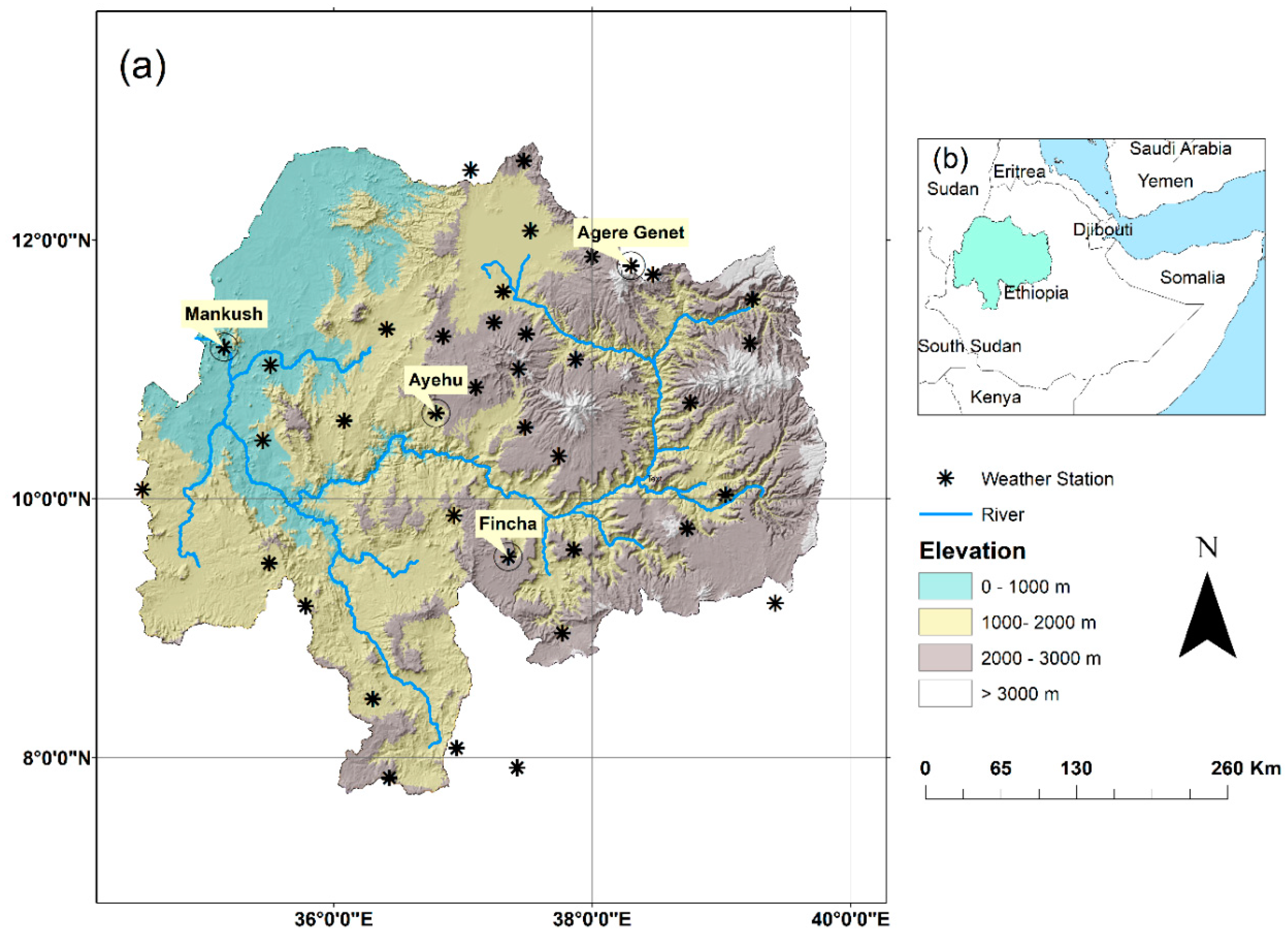
2.1. Study Area

UBNRB is one of the 11 river basins of Ethiopia. It is located between the 7°40′ and 2°50′ N latitude and 36°40′ and 39°40′ longitude (Figure 1). With its 176,000 km2 catchment area [22], it drains the northwest highlands of the country. The Blue Nile River (locally known as Abbay) originates from Lake Tana (area 3060 km2), passes through rugged terrains, and finally crosses the Ethio-Sudan border to join the White Nile near Khartoum, Sudan. The basin contributes about 60% of the annual flow of the Nile [23]. The basin is characterized by diverse topography with the altitude ranging from 500 to 4160 m.a.s.l. The climate is also highly variable both in spatial and temporal scales [24,25]. The basin receives its highest precipitation during the main rainfall season, which occurs from June to September. It also receives significant precipitation during the short rainy season, which runs from March to May. The mean annual rainfall of the basin spans from 1200 mm in the southwest section to 1600 mm in the northeast [26].

2.2. Datasets

In this study, a comparison was made for three (IMERG6, MSWEP2.2, and SM2RAIN-ASCAT1.1) state of the art, and high-resolution gridded datasets against gauge observations over UBNRB for the period of 2007 to 2016. The datasets are chosen due to their unique approaches and distinct input sources to estimate precipitation.
A total of 38 relatively good quality rain gauge data were collected from the Ethiopian National Meteorology Agency (NMA). The gauges were selected to get the best available spatial and temporal coverage over the basin. Rigorous quality checking has been performed on gauge records. These include assessment of the number of missing data from each station, outlier detection, and homogeneity checks. The percentage of missing data for the study period was calculated by dividing the number of missing daily records by the total number of days. The presence of outliers was checked by comparing the observation of a given day with observations of other years but in the same month. The double mass curve technique was applied to check each station’s consistency and homogeneity following the procedure outlined in [27]. Based on the quality checking procedures, stations with more than 5% missing data over the study period were discarded. Consequently, the analysis period was fixed between the years 2007 and 2016. Locations of gauges and elevation information of UBNRB is shown in Figure 1.
Additionally, we also included the CHIRPS2 and Enhancing National Climate Services (ENACTS; [28]) datasets for comparison purposes as they are highly successful products over Ethiopia in general and the UBNRB in particular [6,18,28,29]. The general overview and description of the datasets used are presented in Table 1.
The procedure followed in this study involves data acquisition, quality control, resampling of ENACTS and CHIRPS2, and computations of continuous and categorical indices. For data analysis and visualization, Python version 3.8.2 (Python Software Foundation, Wilmington, Delaware, United States. https://www.python.org/psf-landing/) is used along with packages such as Pandas (https://pandas.pydata.org), NumPy (https://www.numpy.org), Matplotlib (https://matplotlib.org), and rioxarray (https://github.com/corteva/rioxarray).

2.3. Data Comparison

No sub-daily records are available for gauge, ENACTS and SM2RAIN-ASCAT1.1 dataset. Additionally, since most hydrologic applications require daily scale precipitation forcing [9,30,31,32], our comparison was limited to daily and lower resolutions (monthly and seasonal). Sub-daily comparisons were not performed in this study. The four standard meteorological seasons used in this study are December to February (DJF), March to May (MAM), June to August (JJA), and September to November (SON).
For consistent comparison, both ENACTS and CHIRPS2 have been upscaled to a common spatial resolution of 0.1° from 0.0375° and 0.05°, respectively. A bilinear interpolation has been applied to transfer daily values from the high-resolution cells to each 0.1° raster cells.
We considered a point-to-pixel comparison in this study. Each rain gauge station was assumed to be representative of the corresponding grid location of each precipitation datasets. Such comparisons are common in evaluating precipitation products against gauge observations [16,30,33]. Given the low density of rain gauges and complex topography of the study area, we decided not to interpolate gauge observations. Hence, a grid-to-grid comparison was not conducted.
Following [9], five rainfall intensity classes have been used to assess the skills of the precipitation datasets. The classes are: no rain (<1 mm/day), light rain (≥1 and <5 mm/day), moderate rain (≥5 and <20 mm/day), heavy rain (≥20 and <40 mm/day), and violent rain (≥40 mm/day).

2.4. Performance Indices

The performances of precipitation datasets used in this study were evaluated using continuous and categorical indices. The continuous measure adopted is the modified Kling-Gupta efficiency (KGE’) [34,35] and its associated components: correlation (r), bias ratio (β), and variability ratio (γ). This measure is proved to be useful in various validation studies as it summarizes the assessment of temporal rainfall dynamics, dry and wet biases, and dispersion using a single metric: the KGE’ [5,9,30,34,35]. Equations to compute KGE’ and its components are given in Appendix A. Optimum value for linear correlation term (r) is unity with a correlation value of zero, indicating the absence of correlation. Similarly, bias ratio (β) and variability ratio (γ) have unity as their optimum value. Consequently, KGE’ also has an optimum value of unity.
Four categorical indices were used to determine the detection capacity of the precipitation datasets: the probability of detection (POD), false alarm ratio (FAR), critical success index (CSI), and frequency bias (fBIAS). POD measures the ability of precipitation datasets to correctly detect gauge readings whereas, FAR measures the proportion of false precipitations provided by the datasets but never recorded by rain gauges. CSI combines measures of POD and FAR to provide a summarized skill measure. fBIAS, on the other hand, measures the skill of each dataset in reproducing the frequency of precipitation events. The indices were applied to assess the ability of daily precipitations and the various intensity classes described in Section 2.3. Equations to compute the categorical indices are given in Appendix A. Except for the FAR, all other measures have an optimum value of unity. FAR values close to zero indicate better skill with zero indicating a perfect skill.

3. Results and Discussions

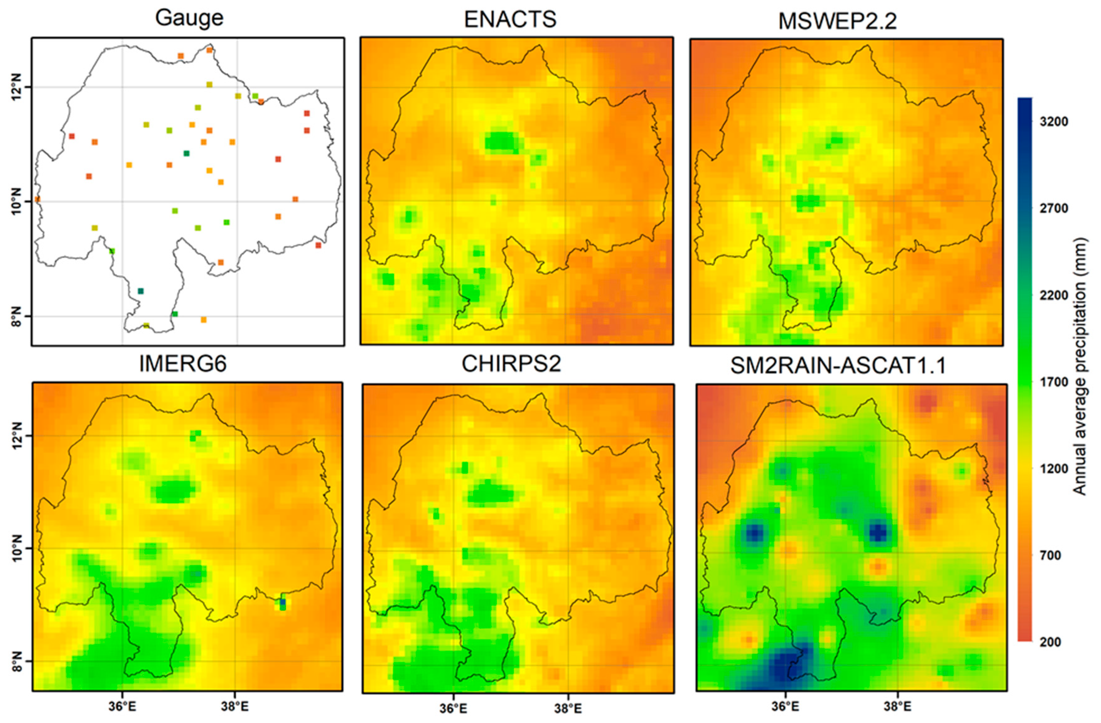
3.1. Representation of Spatial Variability

Representation of spatial variability of precipitation is one key element in assessing the skills of precipitation datasets. Terrain elevation determines the magnitude and distribution of rainfall and other interacting factors such as terrain slope and aspect [36]. Based on the 38-gauge stations used in this study, the mean annual precipitation of UBNRB varies between 422 and 2539 mm during 2007 to 2016, with a decreasing pattern from southwest to northeast. This pattern was in agreement with the finding reported in [37]. Figure 2 shows the annual average precipitations of gauge observations and gridded precipitation estimations for 2007 to 2016 over UBNRB. All datasets except SM2RAIN-ASCAT1.1 similarly represented southwest and central regions of high rainfall and low northwest and eastern rainfalls. As ENACTS used more than 500 quality-controlled gauge observations of Ethiopia in its data generation procedure, we used it as a reference to visually compare the other gridded datasets. Consequently, CHIRPS2, followed by MSWEP2.2, captured the precipitation pattern of UBNRB well. They captured the decreasing southwest to northeast precipitation trend adequately. SM2RAIN-ASCAT1.1, on the other hand, provides the worst performance with substantial overestimations in most areas. The poor performance of SM2RAIN-ASCAT1.1 could be due to the presence of spurious rainfall events as a result of high-frequency soil moisture fluctuations. According to [21], the Advanced SCATterometer (ASCAT) soil moisture dataset contains false soil moisture signals due to measurement and retrieval errors. Such false signals are especially apparent in topographically complex areas. As a result, the retrieval algorithm named soil moisture to rain (SM2RAIN) misinterprets these false soil moisture signals as rainfall.
Terrain elevation and orientation highly affect the characteristics of precipitation distributions. Median values of the validation results across various elevation ranges for a daily time scale over UBNRB is given in Table 2. In general, the performance was low for all precipitation datasets except for ENACTS. The poor performance could be due to the apparent difficulties in capturing variabilities at high temporal scales, such as daily. These difficulties could lead to large uncertainties in daily precipitation estimations. Since ENACTS incorporates many high-quality gauged data, a higher linear correlation and KGE’ was observed, especially in elevations higher than 1500 m.a.s.l.
Furthermore, the ENACTS performance was similar in these higher elevations indicating the minor influence of altitude on ENACTS estimations’ skill. All other datasets scored a linear correlation (r) less than 0.6 and a KGE’ less than 0.5, indicating their limitation to reproduce the spatial characteristics of daily precipitation at each elevation range. However, the linear correlation of these datasets shows a general increasing trend with an increase in elevation. The precipitation variability was also accurately represented by ENACTS, although CHIRPS2 and IMERG6 slightly outperformed it on the last two higher elevation classes. SM2RAIN-ASCAT1.1 poorly represented spatial variability of daily precipitation over UBNRB with a general score of around γ = 0.5. CHIRPS2 exhibits a consistent and minimal bias in all elevation categories.
As shown in Figure 3, the skill of precipitation datasets has improved on the monthly time scale. As expected, the improvement was based on the cancellation of positive and negative errors on a daily scale following the aggregation to a monthly scale. A higher correlation (r > 0.85) has been achieved by each dataset, indicating a good agreement between rain gauge observations and gridded estimations. Furthermore, the elevation difference appeared not to affect the correlation significantly. Consequently, the datasets were able to capture the local convective fluctuations at a monthly scale properly. Most of the precipitation datasets resulted in a bias ratio close to the perfect score of one across each elevation range, whereas SM2RAIN-ASCAT1.1 showed a considerable wet bias, especially for elevations higher than 1500 m.a.s.l. A possible explanation for this overestimation could be erroneous soil moisture signals in ASCAT observations, which ultimately led to interpreting these wrong signals as rainfall by the SM2RAIN algorithm [21,38]. Precipitation variability was nicely reproduced by all datasets within the range of γ = 0.8 and γ = 1.1 for all elevation levels. Except for SM2RAIN-ASCAT1.1, the pattern of KGE’ looks similar for the elevations higher than 1500 m.a.s.l. For SM2RAIN-ASCAT1.1, KGE’ decreases with an increase in elevation. CHIRPS2 (KGE’ > 0.86) generally performed better in each elevation range followed by IMERG6 (KGE’ > 0.83). The overall monthly skill of ENACTS (KGE’ > 0.79) was low compared to CHIRPS2 and IMERG6. The general low daily and monthly skills of SM2RAIN-ASCAT1.1 in reproducing the precipitation characteristics of UBNRB (Table 2 and Figure 3) make it less applicable in the region.
Apart from continuous indices such as the modified Kling-Gupta efficiency and its components, categorical indices are also good indicators of the skills of precipitation datasets [5,9]. They are useful to assess the detection capacity of the datasets concisely. Figure 4 illustrates the categorical indices of the precipitation datasets compared to gauge observations for 2007 to 2016 over the various elevation classes of UBNRB. All datasets except ENACTS and CHIRPS2 showed a consistent and higher than 0.9 probability of detection (POD) at all elevation levels. ENACTS had an overall detection score between POD = 0.7 and POD = 0.9. CHIRPS2, on the other hand, has shown a POD comparable to ENACTS for elevations less than 1550 m.a.s.l. and a decreasing score on higher elevations after that. Therefore, CHIRPS2 showed the weakest ability in detecting daily gauge observations, especially on those elevations higher than 1500 m.a.s.l. Although physiographic information is included in the data generation process of CHIRPS2 [17], that did not help to capture daily gauge records accurately. Based on the false alarm ratio (FAR) results, ENACTS provided a consistent skill at all elevation levels (FAR between 0 and 0.2). CHIRPS2, MSWEP2.2, and IMERG6 have shown the next better FAR within the range of 0.2 to 0.4. SM2RAIN-ASCAT1.1 exhibited the least performance, according to FAR. The FAR analysis further revealed that the skill of ENACTS and CHIRPS2 tended to improve with an increase in elevation while IMERG6 and MSWEP2.2 seemed to be unaffected by the variation in elevation. SM2RAIN-ASCAT1.1, on the other hand, showed no clear relationship with elevation. Again, with the possibility of SM2RAIN algorithm’s limitation to differentiate incorrect soil moisture signals of ASCAT sensors, there were superfluous precipitation values present in SM2RAIN-ASCAT1.1, which led to its exaggerated false alarms. A higher critical success index (CSI) was observed for ENACTS (CSI > 0.5). MSWEP2.2 and IMERG6 showed the next good CSI score indicating a better detection probability and provision of relatively low false precipitations compared to gauge observations. CSI values of SM2RAIN-ASCAT1.1 fluctuate between 0.3 and 0.6, indicating its poor performance. CSI scores seem to be unaffected by elevation differences for all precipitation datasets. ENACTS and CHIRPS2 tended to underestimate the frequency of precipitation events while others overestimated it slightly. The best score of fBIAS was provided by ENACTS followed by CHIRPS2 and IMERG6, whereas SM2RAIN-ASCAT1.1 scored the least fBIAS. In general, ENACTS showed superior performance in most validation tools. This success could be attributed to the inclusion of numerous quality controlled gauge observations and other proxies such as elevation information during data development [28]. Incorrect interpretations of soil moisture by the SM2RAIN algorithm could cause the relatively poor performance of SM2RAIN-ASCAT1.1. Categorical indices of IMERG6 and MSWEP2.2 show a general resistance to vary with elevation, indicating the datasets’ ability to capture local climate fluctuations in different regions of UBNRB correctly.

3.2. Representation of Temporal Variability

Figure 5, Figure 6, Figure 7 and Figure 8 show boxplots of KGE’ and associated components (r, β, and γ) for each precipitation dataset and different temporal scales (daily, monthly, and four seasons).
Figure 5 shows a linear correlation (r) between gauge values and each dataset’s corresponding grid cells. On a daily scale, it is clear that ENACTS performed better (median r = 0.82) than others. The other datasets scored low linear correlation values in the range of 0.4 to 0.5, showing a similar and lower performance in representing the overall daily precipitation dynamics. For a better visual inspection of the correlation at a daily time step, a scatter plot is presented in Figure 9. On a monthly scale, however, a higher score (r > 0.9) was achieved by all datasets. ENACTS provided the highest monthly median correlation (r = 0.95) followed by CHIRPS2 (r = 0.93) and IMERG6 (r = 0.93). On a seasonal scale, all datasets represented the short rainy season (MAM) of UBNRB well. Except for IMERG6 (median r = 0.64), all other datasets yielded a correlation of more than 0.7 for this season. In other seasons (DJF, JJA, and SON), the datasets exhibited a lower and more or less similar performance.
Figure 6 illustrates the bias ratio (β) of precipitation datasets on different time scales compared to gauge observations. The performance was similar at daily and monthly time steps in which SM2RAIN-ASCAT1.1 showed considerable overestimation while others were nearly unbiased. Despite the consistent overestimation of SM2RAIN-ASCAT1.1, all other precipitation datasets performed well in MAM, JJA, and SON seasons. All datasets performed worst in the dry season (DJF).
In Figure 7, the variability ratio (γ) of the various precipitation datasets compared to gauge observations for different temporal scales is presented. All precipitation datasets reproduced the precipitation variability correctly both on daily and monthly scales. However, SM2RAIN-ASCAT1.1 tended to underestimate the daily precipitation variability (median γ = 0.52). Except for ENACTS, all other datasets tended to underestimate the variability in all seasons, with the most considerable underestimation scored by CHIRPS2 (median γ = 0.46) in the DJF season. ENACTS exhibited a slight overestimation for each season. Compared to other seasons, DJF overestimation of ENACTS was more considerable (median γ = 1.2).
Figure 8 shows the overall KGE’ of the precipitation datasets, which essentially summarizes their correlation, bias, and variabilities compared to gauge observations. On a daily scale, ENACTS showed a better performance with a median KGE’ of 0.75. On the same daily scale, all other datasets’ KGE’ values tend to fluctuate between 0 and 0.5, indicating limited overall performance. The performance of CHIRPS2, IMERG6, and MSWEP2.2 was highly improved when aggregated to the monthly time scale, leaving SM2RAIN-ASCAT1.1 as the worst performer (median KGE’ = 0.56). All datasets performed better in the MAM season (median KGE’ > 0.5) while they all performed worst in DJF season (median KGE’ < 0.3). In JJA and SON seasons, SM2RAIN-ASCAT1.1 showed low skill (median KGE’ < 0.1) while others showed mixed performance with KGE’ ranging between 0.11 and 0.83. In general, ENACTS showed an overall better performance, followed by CHIRPS2. SM2RAIN-ASCAT1.1 remained the worst. Seasonally, a better score is achieved for wet seasons (MAM and JJA) than the dry seasons (DJF and SON) by most datasets.
An example scatter plot is given in Figure 9 to illustrate the relationship between daily gauge observations and the corresponding precipitation datasets. ENACTS has shown the best agreement with gauge observations (with r = 0.86). The other datasets exhibited a similar skill with a coefficient of correlation ranging between 0.55 and 0.6. The difference between gauge observations and dataset estimations increases as the magnitude of precipitation increases. Generally, the agreement was better for precipitation amounts below 25 mm, and the discrepancy increases after that. Compared to others, CHIRPS2 exhibited the lowest agreement with gauge observations (r = 0.55).
Time series plots are provided in Figure 10 to examine the relationship between gauge observations and gridded estimations further. The plots show each precipitation dataset’s monthly time series relationship for selected gauge locations for the period of 2007 to 2016 (Figure 1). The stations were selected to ensure that each of the five elevation classes used in this study were represented. As a result, the agreement between gauge observations and precipitation datasets was better for the Mankush station (1020 m.a.s.l). A similar good agreement was observed at Ayehu (1725 m.a.s.l) and Fincha (2262 m.a.s.l). SM2RAIN-ASCAT1.1, however, showed significant overestimations of the monthly peak precipitations at both the Ayehu and Fincha stations. Furthermore, at Fincha station, SM2RAIN-ASCAT1.1 overestimated the monthly low precipitation values as well. At the Agere Genet station (3010 m.a.s.l), which has the highest elevation among the 38 stations considered in this study, SM2RAIN-ASCAT1.1 overestimated the monthly peak as well as low precipitation values. The difference between SM2RAIN-ASCAT1.1 estimation and gauge observation turned as high as 1195 mm/month for this specific station. The results are in agreement with the findings discussed in Section 3.1.

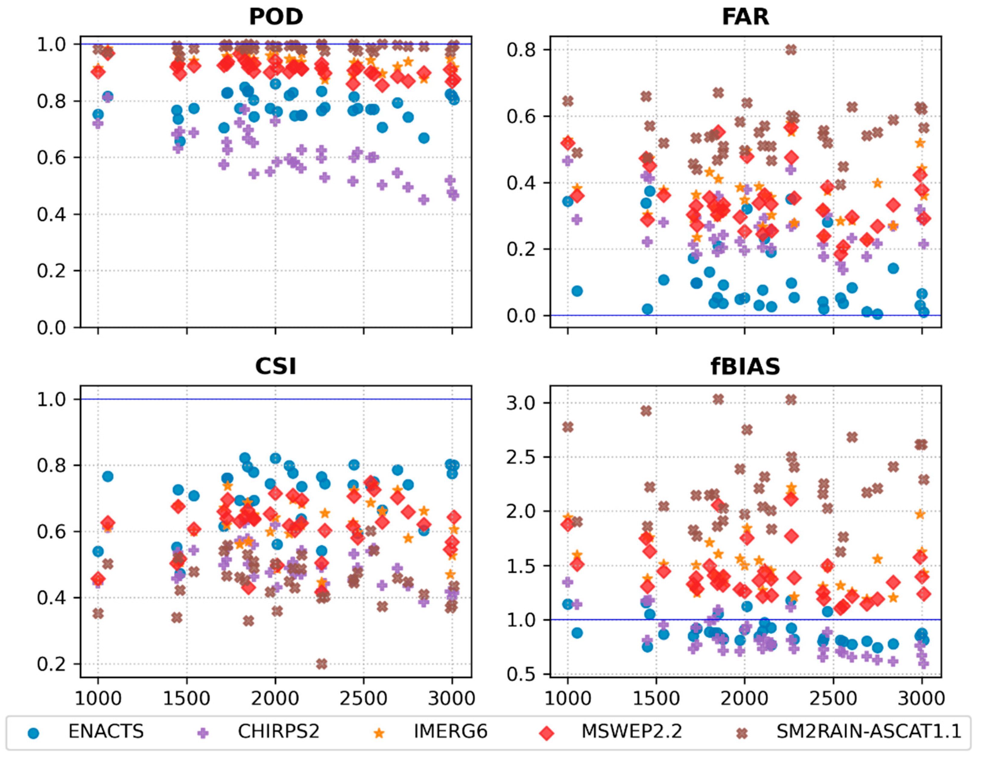
3.3. Representation of Different Intensities

Table 3 presents the median values of the categorical indices obtained from precipitation datasets for 2007 to 2016 categorized by the five precipitation intensity classes. For a no rain condition, all datasets performed well despite the relatively low skills of SM2RAIN-ASCAT1.1. Generally, the skill of precipitation datasets decreases with an increase in precipitation intensity. A general overestimation of light and moderate precipitation events is observed. Furthermore, heavy and violent precipitation events were underestimated by most datasets. ENACTS offered the best bias estimation for events below 40 mm/day, while IMERG6 showed the best bias estimate for precipitation events of more than 40 mm/day. SM2RAIN-ASCAT1.1, followed by IMERG6 and MSWEP2.2, also observed a significantly high overestimation of light rain events.

4. Conclusions

The main objectives of this study were to evaluate the skills of precipitation estimates from three different sources: IMERG6, MSWEP2.2, and SM2RAIN-ASCAT1.1. The comparison was made with rain gauge observations and two other high-resolution precipitation datasets: ENACTS and CHIRPS2. Along the way, we validated CHIRPS2 and ENACTS products as well. The modified Kling-Gupta efficiency (KGE’) and four categorical indices (POD, FAR, CSI, and fBIAS) were used to measure each dataset’s skills over UBNRB for the period of 2007 to 2016. Based on the findings of this study, ENACTS showed a superior performance followed by CHIRPS2. IMERG6 and MSWEP2.2 show the next best performance behaving similarly for most measures. The inclusion of extensive gauge observations, compared to others, helped ENACTS to achieve the best performance, whereas the high-resolution nature of CHIRPS2 enabled it to capture local climate variations well. SM2RAIN-ASCAT1.1 shows the least performance everywhere due to problems that could be associated with misinterpretations of soil moisture signals by the SM2RAIN algorithm. All datasets, except ENACTS, performed poorly on daily scale measures. Their skill, however, improves on a monthly scale but with a decreasing performance at elevations higher than 1500 m.a.s.l.
The results obtained show that:
  • CHIRPS2, IMERG6, and MSWEP2.2 precipitations exhibit good agreement with the average annual rainfall from ENACTS and the gauge dataset.
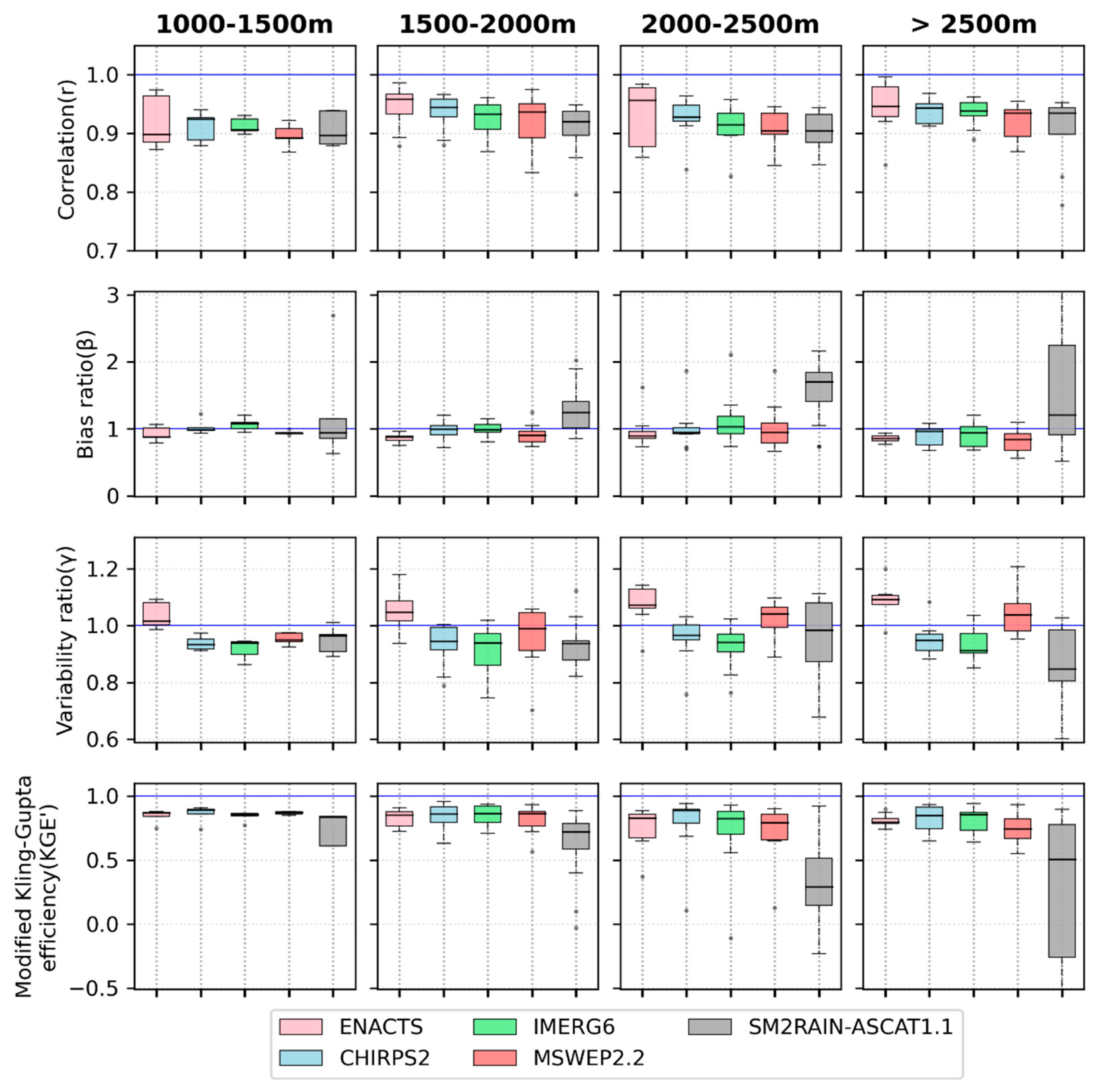
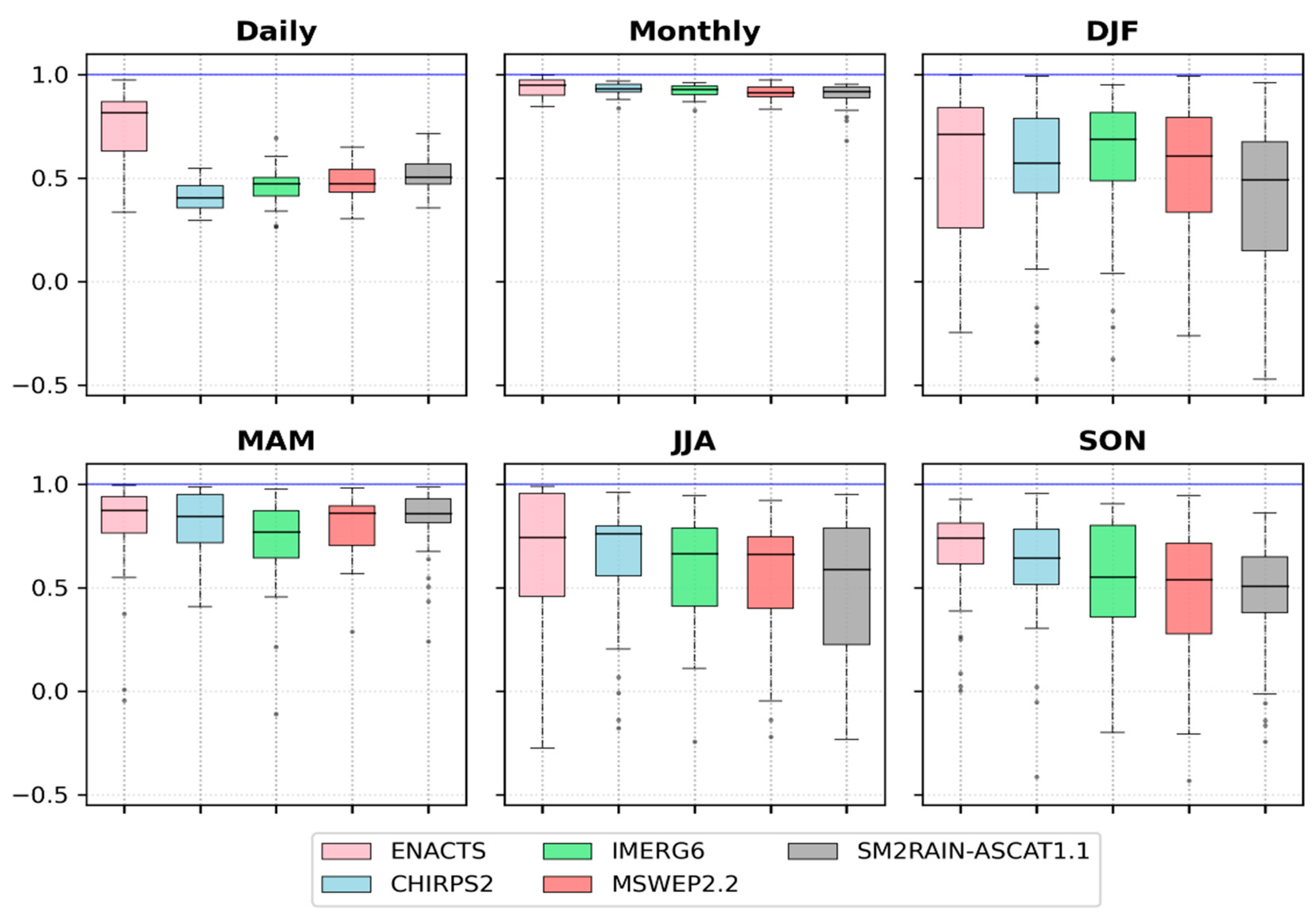
  • All datasets provided better linear correlation (median r > 0.5) for monthly and seasonal time scales with the best correlation at the monthly time step (median r > 0.9).
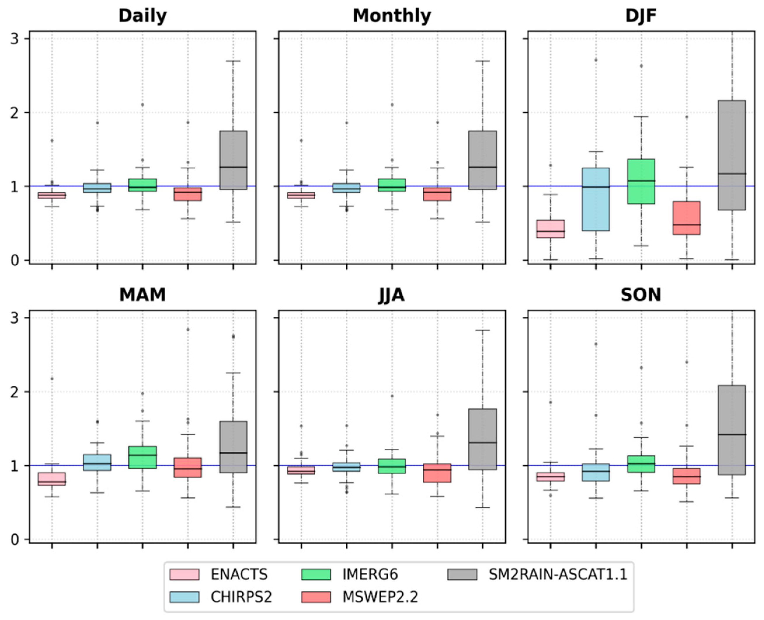
  • All datasets except SM2RAIN-ASCAT1.1 were nearly unbiased at all time scales except the dry season (DJF). SM2RAIN-ASCAT1.1 consistently and significantly overestimated the precipitation compared to gauge observations.
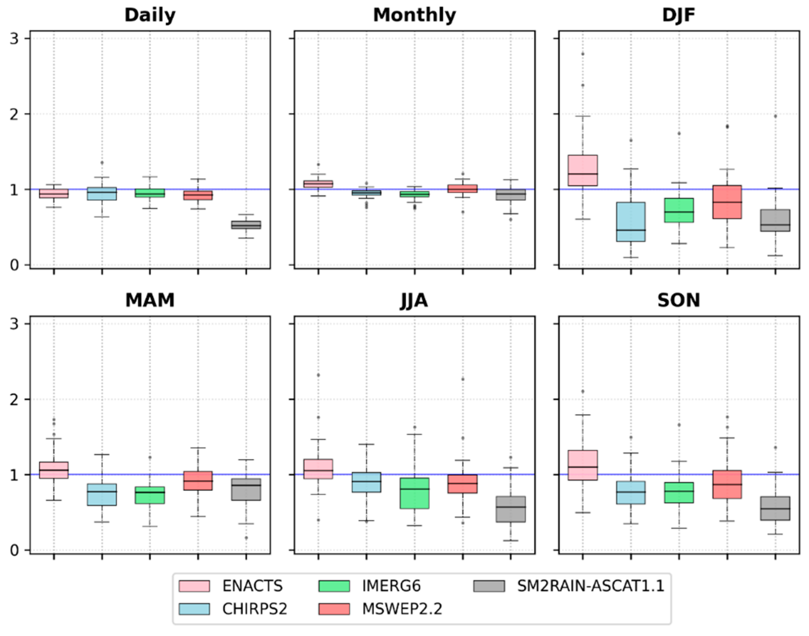
  • All datasets captured precipitation variability on daily and monthly scales despite SM2RAIN-ASCAT1.1′s relatively low skill on a daily scale. A similar underestimation of precipitation variability has been observed at MAM, JJA, and SON seasons by all datasets. ENACTS, in contrast, showed a slight overestimation.
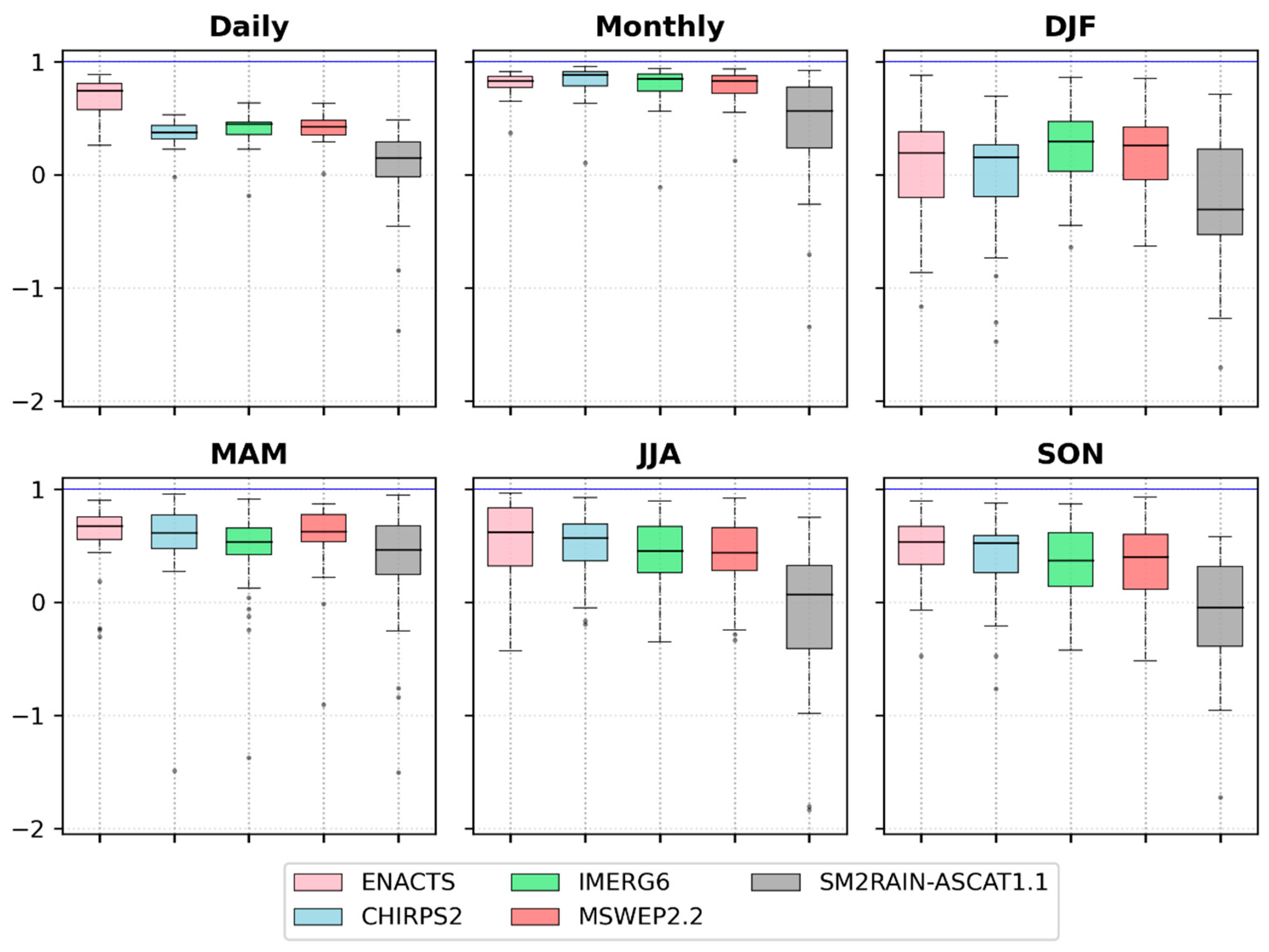
  • Based on KGE’, all datasets had the best skill on a monthly time scale. On the remaining times, the overall performance was poor.
  • ENACTS, MSWEP2.2, and IMERG6 showed better success (CSI > 0.6) in detecting precipitation at different elevations. As evidenced by all categorical measures, the resistance of MSWEP2.2 and IMERG6 to the influence of elevation variation shows their strength in correctly representing the area’s local climate features.
  • All datasets correctly identified the occurrence of no-rain events (<1 mm/day). However, for higher intensities, they presented a low and deteriorating skill with an increase in intensity.
  • Considering the scarcity of gauged datasets over UBNRB, IMERG6 and MSWEP2.2 could be considered to be valuable datasets for hydro-climatic analysis, particularly where gauging density is low. SM2RAIN-ASCAT1.1, on the other hand, needs a critical correction to treat its apparent wet biases before use.

Author Contributions

Conceptualization, S.A.A. and D.Y.; methodology, S.A.A., D.Y., and T.Q.; formal analysis, S.A.A.; investigation, S.A.A. and D.Y.; data curation, E.B.G. and H.T.W.; writing—original draft preparation, S.A.A. and T.Q.; writing—review and editing, D.Y., E.B.G., H.T.W., W.K., S.L., and B.D.; visualization, E.B.G., W.K., S.L., and B.D.; funding acquisition, D.Y. All authors have read and agreed to the published version of the manuscript.

Funding

This research was supported by the National Key Research and Development Project (Grant No. 2016YFA0601503 and 2017YFA0605004) and the National Science Fund for Distinguished Young Scholars (Grant No. 51725905).

Acknowledgments

We would like to thank the National Meteorological Agency of Ethiopia for the gauge observation and ENACTS data used in this study. We are also grateful to the data providers of CHIRPS, IMERG, MSWEP, and SM2RAIN-ASCAT.

Conflicts of Interest

The authors declare no conflict of interest.

Appendix A. Continuous and Categorical Indices Used for Evaluation

  • Continuous indices
    • Modified Kling-Gupta efficiency (KGE’)
      1 ( r 1 ) 2 + ( β 1 ) 2 + ( γ 1 ) 2
    • Pearson correlation coefficient (r)
      r =   i = 1 n ( x i x ¯ ) ( y i y ¯ ) i = 1 n ( x i x ¯ ) 2 i = 1 n ( y i y ¯ ) 2
    • Bias ratio (β)
      β =   y ¯ x ¯
    • Variability ratio (γ)
      γ =   s y y ¯ s x x ¯
      where x = gauge observation, y = estimated precipitation, n = number of observations, x ¯ = average gauge observation, y ¯ = average estimated precipitation, sx = standard deviation of gauge observations, sy = standard deviation of estimated precipitations.
  • Categorical indices
    e.
    Probability of detection (POD)
    H H + M
    f.
    False alarm ratio (FAR)
    F A H + F A
    g.
    Critical success index (CSI)
    H. H + F A + M
    h.
    Frequency bias (fBIAS)
    H + F A H + M
    where H = hit (number of gauge observations correctly detected by datasets), M = miss (number of gauge observations which are not correctly detected by datasets), FA = false alarm (number of false precipitations recorded by datasets but not at the gauge).

References

  1. Beven, K.J. Rainfall-Runoff Modelling: The Primer, 2nd ed.; Wiley-Blackwell: Chichester, West Sussex, UK; Hoboken, NJ, USA, 2012; ISBN 978-0-470-71459-1. [Google Scholar]
  2. Artan, G.; Gadain, H.; Smith, J.L.; Asante, K.; Bandaragoda, C.J.; Verdin, J.P. Adequacy of satellite derived rainfall data for stream flow modeling. Nat. Hazards 2007, 43, 167–185. [Google Scholar] [CrossRef]
  3. Behrangi, A.; Khakbaz, B.; Jaw, T.C.; AghaKouchak, A.; Hsu, K.; Sorooshian, S. Hydrologic evaluation of satellite precipitation products over a mid-size basin. J. Hydrol. 2011, 397, 225–237. [Google Scholar] [CrossRef] [Green Version]
  4. Sun, Q.; Miao, C.; Duan, Q.; Ashouri, H.; Sorooshian, S.; Hsu, K. A Review of Global Precipitation Data Sets: Data Sources, Estimation, and Intercomparisons. Rev. Geophys. 2018, 56, 79–107. [Google Scholar] [CrossRef] [Green Version]
  5. Acharya, S.C.; Nathan, R.; Wang, Q.J.; Su, C.-H.; Eizenberg, N. An evaluation of daily precipitation from a regional atmospheric reanalysis over Australia. Hydrol. Earth Syst. Sci. 2019, 23, 3387–3403. [Google Scholar] [CrossRef] [Green Version]
  6. Ayehu, G.T.; Tadesse, T.; Gessesse, B.; Dinku, T. Validation of new satellite rainfall products over the Upper Blue Nile Basin, Ethiopia. Atmospheric Meas. Tech. 2018, 11, 1921–1936. [Google Scholar] [CrossRef] [Green Version]
  7. Dinku, T.; Chidzambwa, S.; Ceccato, P.; Connor, S.J.; Ropelewski, C.F. Validation of high-resolution satellite rainfall products over complex terrain. Int. J. Remote Sens. 2008, 29, 4097–4110. [Google Scholar] [CrossRef]
  8. Gebremichael, M.; Bitew, M.M.; Hirpa, F.A.; Tesfay, G.N. Accuracy of satellite rainfall estimates in the Blue Nile Basin: Lowland plain versus highland mountain. Water Resour. Res. 2014, 50, 8775–8790. [Google Scholar] [CrossRef]
  9. Zambrano-Bigiarini, M.; Nauditt, A.; Birkel, C.; Verbist, K.; Ribbe, L. Temporal and spatial evaluation of satellite-based rainfall estimates across the complex topographical and climatic gradients of Chile. Hydrol. Earth Syst. Sci. 2017, 21, 1295–1320. [Google Scholar] [CrossRef] [Green Version]
  10. Conway, D.; Mould, C.; Bewket, W. Over one century of rainfall and temperature observations in Addis Ababa, Ethiopia. Int. J. Clim. 2004, 24, 77–91. [Google Scholar] [CrossRef]
  11. Abera, W.; Brocca, L.; Rigon, R. Comparative evaluation of different satellite rainfall estimation products and bias correction in the Upper Blue Nile (UBN) basin. Atmospheric Res. 2016, 471–483. [Google Scholar] [CrossRef]
  12. Lakew, H.B.; Moges, S.; Asfaw, D.H. Hydrological Evaluation of Satellite and Reanalysis Precipitation Products in the Upper Blue Nile Basin: A Case Study of Gilgel Abbay. Hydrology 2017, 4, 39. [Google Scholar] [CrossRef] [Green Version]
  13. Dinku, T.; Connor, S.; Ceccato, P. Evaluation of Satellite Rainfall Estimates and Gridded Gauge Products over the Upper Blue Nile Region. In Nile River Basin; Melesse, A.M., Ed.; Springer: Dordrecht, The Netherlands, 2011; pp. 109–127. ISBN 978-94-007-0688-0. [Google Scholar]
  14. Fenta, A.A.; Rientjes, T.; Haile, A.T.; Reggiani, P. Satellite Rainfall Products and Their Reliability in the Blue Nile Basin. In Nile River Basin; Melesse, A.M., Abtew, W., Setegn, S.G., Eds.; Springer International Publishing: Cham, Switzerland, 2014; pp. 51–67. ISBN 978-3-319-02719-7. [Google Scholar]
  15. Lakew, H.B.; Moges, S.A.; Asfaw, D.H. Hydrological performance evaluation of multiple satellite precipitation products in the upper Blue Nile basin, Ethiopia. J. Hydrol. Reg. Stud. 2020, 27, 100664. [Google Scholar] [CrossRef]
  16. Worqlul, A.W.; Maathuis, B.; Adem, A.A.; Demissie, S.S.; Langan, S.; Steenhuis, T.S. Comparison of rainfall estimations by TRMM 3B42, MPEG and CFSR with ground-observed data for the Lake Tana basin in Ethiopia. Hydrol. Earth Syst. Sci. 2014, 18, 4871–4881. [Google Scholar] [CrossRef] [Green Version]
  17. Funk, C.; Peterson, P.; Landsfeld, M.; Pedreros, D.; Verdin, J.; Shukla, S.; Husak, G.; Rowland, J.; Harrison, L.; Hoell, A.; et al. The climate hazards infrared precipitation with stations—A new environmental record for monitoring extremes. Sci. Data 2015, 2, 150066. [Google Scholar] [CrossRef] [PubMed] [Green Version]
  18. Dinku, T.; Funk, C.; Peterson, P.; Maidment, R.; Tadesse, T.; Gadain, H.; Ceccato, P. Validation of the CHIRPS satellite rainfall estimates over eastern Africa. Q. J. R. Meteorol. Soc. 2018, 144, 292–312. [Google Scholar] [CrossRef] [Green Version]
  19. Huffman, G.J.; Bolvin, D.T.; Braithwaite, D.; Hsu, K.; Joyce, R.; Kidd, C.; Nelkin, E.J.; Sorooshian, S.; Tan, J.; Xie, P. Algorithm Theoretical Basis Document (ATBD) Version 6 for the NASA Global Precipitation Measurement (GPM) Integrated Multi-satellitE Retrievals for GPM (IMERG) GPM Project, Greenbelt, MD. 2019. Available online: https://gpm.nasa.gov/sites/default/files/document_files/IMERG_ATBD_V06.pdf (accessed on 30 October 2020).
  20. Beck, H.E.; Wood, E.F.; Pan, M.; Fisher, C.K.; Miralles, D.G.; Van Dijk, A.I.J.M.; McVicar, T.R.; Adler, R.F. MSWEP V2 Global 3-Hourly 0.1° Precipitation: Methodology and Quantitative Assessment. Bull. Am. Meteorol. Soc. 2019, 100, 473–500. [Google Scholar] [CrossRef] [Green Version]
  21. Brocca, L.; Filippucci, P.; Hahn, S.; Ciabatta, L.; Massari, C.; Camici, S.; Schüller, L.; Bojkov, B.; Wagner, W. SM2RAIN–ASCAT (2007–2018): Global daily satellite rainfall data from ASCAT soil moisture observations. Earth Syst. Sci. Data 2019, 11, 1583–1601. [Google Scholar] [CrossRef] [Green Version]
  22. Conway, D. The Climate and Hydrology of the Upper Blue Nile River. Geogr. J. 2000, 166, 49–62. [Google Scholar] [CrossRef] [Green Version]
  23. Conway, D. From headwater tributaries to international river: Observing and adapting to climate variability and change in the Nile basin. Glob. Environ. Chang. 2005, 15, 99–114. [Google Scholar] [CrossRef]
  24. Abtew, W.; Melesse, A.M.; Dessalegne, T. Spatial, inter and intra-annual variability of the Upper Blue Nile Basin rainfall. Hydrol. Process. 2009, 23, 3075–3082. [Google Scholar] [CrossRef]
  25. Samy, A.; Ibrahim, M.G.; Mahmod, W.E.; Fujii, M.; Eltawil, A.; Daoud, W. Statistical Assessment of Rainfall Characteristics in Upper Blue Nile Basin over the Period from 1953 to 2014. Water 2019, 11, 468. [Google Scholar] [CrossRef] [Green Version]
  26. Kim, U.; Kaluarachchi, J.J.; Smakhtin, V.U. Generation of Monthly Precipitation Under Climate Change for the Upper Blue Nile River Basin, Ethiopia1. JAWRA J. Am. Water Resour. Assoc. 2008, 44, 1231–1247. [Google Scholar] [CrossRef]
  27. Searcy, J.K.; Hardison, C.H.; Langbein, W.B. Double-Mass Curves, with a Section Fitting Curves to Cyclic Data; U.S. Government Printing Office: Washington, DC, USA, 1960.
  28. Dinku, T.; Block, P.; Sharoff, J.; Hailemariam, K.; Osgood, D.; Del Corral, J.; Cousin, R.; Thomson, M.C. Bridging critical gaps in climate services and applications in africa. Earth Perspect. 2014, 1, 15. [Google Scholar] [CrossRef] [Green Version]
  29. Bayissa, Y.; Tadesse, T.; Demisse, G.; Shiferaw, A. Evaluation of Satellite-Based Rainfall Estimates and Application to Monitor Meteorological Drought for the Upper Blue Nile Basin, Ethiopia. Remote Sens. 2017, 9, 669. [Google Scholar] [CrossRef] [Green Version]
  30. Baez-Villanueva, O.M.; Zambrano-Bigiarini, M.; Ribbe, L.; Nauditt, A.; Giraldo-Osorio, J.D.; Thinh, N.X. Temporal and spatial evaluation of satellite rainfall estimates over different regions in Latin-America. Atmospheric Res. 2018, 213, 34–50. [Google Scholar] [CrossRef]
  31. Gebregiorgis, A.S.; Hossain, F. Understanding the Dependence of Satellite Rainfall Uncertainty on Topography and Climate for Hydrologic Model Simulation. IEEE Trans. Geosci. Remote Sens. 2012, 51, 704–718. [Google Scholar] [CrossRef]
  32. Thiemig, V.; Rojas, R.; Zambrano-Bigiarini, M.; Levizzani, V.; De Roo, A. Validation of Satellite-Based Precipitation Products over Sparsely Gauged African River Basins. J. Hydrometeorol. 2012, 13, 1760–1783. [Google Scholar] [CrossRef]
  33. Su, J.; Lü, H.; Zhu, Y.; Cui, Y.; Wang, X. Evaluating the hydrological utility of latest IMERG products over the Upper Huaihe River Basin, China. Atmospheric Res. 2019, 225, 17–29. [Google Scholar] [CrossRef]
  34. Gupta, H.V.; Kling, H.; Yilmaz, K.K.; Martinez, G.F. Decomposition of the mean squared error and NSE performance criteria: Implications for improving hydrological modelling. J. Hydrol. 2009, 377, 80–91. [Google Scholar] [CrossRef] [Green Version]
  35. Kling, H.; Fuchs, M.; Paulin, M. Runoff conditions in the upper Danube basin under an ensemble of climate change scenarios. J. Hydrol. 2012, 264–277. [Google Scholar] [CrossRef]
  36. Haile, A.T.; Rientjes, T.; Gieske, A.; Gebremichael, M. Rainfall Variability over Mountainous and Adjacent Lake Areas: The Case of Lake Tana Basin at the Source of the Blue Nile River. J. Appl. Meteorol. Clim. 2009, 48, 1696–1717. [Google Scholar] [CrossRef]
  37. Melesse, A.M.; Abtew, W.; Setegn, S.G.; Dessalegne, T. Hydrological Variability and Climate of the Upper Blue Nile River Basin. In Nile River Basin; Melesse, A.M., Ed.; Springer: Dordrecht, The Netherlands, 2011; pp. 3–37. ISBN 978-94-007-0688-0. [Google Scholar]
  38. Brocca, L.; Ciabatta, L.; Massari, C.; Moramarco, T.; Hahn, S.; Hasenauer, S.; Kidd, R.; Dorigo, W.; Wagner, W.; Levizzani, V. Soil as a natural rain gauge: Estimating global rainfall from satellite soil moisture data: Using the soil as a natural raingauge. J. Geophys. Res. Atmos. 2014, 119, 5128–5141. [Google Scholar] [CrossRef]
Figure 1. Study area. (a) Digital elevation map of the Upper Blue Nile River Basin (UBNRB) and the location of 38 selected rain gauges. (b) Inset map showing the location of the study area. Encircled and labeled stations in (a) are used for monthly time series plots in Section 3.2.
Water 12 03072 g001
Figure 2. Mean annual precipitation generated from different datasets over UBNRB.
Water 12 03072 g002
Figure 3. Boxplot of correlation (r), bias ratio (β), variability ratio (γ), and modified Kling-Gupta efficiency (KGE’) values of precipitation datasets compared to gauge observation. The horizontal blue line indicates the respective optimum score for each measure.
Water 12 03072 g003
Figure 4. Categorical indices of precipitation datasets as classified by elevation over UBNRB. From left to right and top to bottom: probability of detection (POD), false alarm ratio (FAR), critical success index (CSI), and frequency bias (fBIAS). The horizontal blue line indicates the respective optimum value for each measure.
Water 12 03072 g004
Figure 5. The linear correlation coefficient (r) between different precipitation datasets and gauge observation at different temporal scales. From left to right and up to bottom: daily, monthly, December to February (DJF), March to May (MAM), June to August (JJA), and September to November (SON). The horizontal blue line indicates the optimum value for r.
Water 12 03072 g005
Figure 6. Bias ratio (β) between different precipitation datasets and gauge observation at different temporal scales. The horizontal blue line indicates the optimum value for β.
Water 12 03072 g006
Figure 7. Variability ratio (γ) between different precipitation datasets and gauge observations on different temporal scales. The horizontal blue line indicates the optimum value for γ.
Water 12 03072 g007
Figure 8. Modified Kling-Gupta efficiency (KGE’) between different precipitation datasets and gauge observations at different temporal scales. The horizontal blue line indicates the optimum value for KGE’.
Water 12 03072 g008
Figure 9. Scatter plots of rain gauge observations and precipitation dataset estimates at daily temporal scale over UBNRB.
Water 12 03072 g009
Figure 10. Monthly scale comparison of the precipitation datasets at selected gauge stations over the UBNRB.
Water 12 03072 g010
Table 1. Overview of precipitation datasets used in this study.
DatasetData SourceSpatial CoverageSpatial ResolutionTemporal ResolutionReferencesDescription
ENACTSGauge and Satellite Selected developing countries0.0375°daily[28]The estimation procedure involves integrating quality-controlled station data with satellite rainfall estimates and other proxies such as elevation information.
CHIRPS2Gauge and Satellite Global0.05°daily, pentad, monthly[17]Data is built by blending Climate Hazard Group’s Infrared Precipitation (CHIRP) with in situ gauge observations.
IMERG6Gauge and Satellite Global0.1°half-hourly, daily, monthly[19]Data is generated by merging passive microwave (PMW) and infrared (IR) precipitations using state of the art calibration and interpolation schemes.
MSWEP2.2Gauge, Satellite and ReanalysisGlobal0.1°three-hourly, daily[20]Estimation follows necessary bias corrections applications, and merging and gauge corrections to selected reanalysis and satellite precipitation estimates.
SM2RAIN-ASCAT1.1Gauge precipitation and Satellite Soil MoistureGlobal0.1°daily[21]The estimation procedure follows the interpolation and filtering of ASCAT observations, followed by applying the soil moisture to rain (SM2RAIN) algorithm and gauge corrections.
Table 2. Daily scale median values of modified Kling-Gupta efficiency (KGE’) and its components grouped for different elevation ranges for UBNRB. The number in brackets indicates the number of stations in the elevation range. Values in bold show the best score of each dataset in each elevation range.
ElevationDatasetCorrelation (r)Bias Ratio (β)Variability Ratio (γ)KGE’
1000–1500 m.a.s.l. (5)ENACTS0.6100.8780.9070.537
CHIRPS20.3520.9840.7260.318
IMERG60.3431.0740.8610.289
MSWEP2.20.4240.9350.8190.382
SM2RAIN-ASCAT1.10.4720.9430.5030.154
1500–2000 m.a.s.l.
(12)
ENACTS0.8110.8790.9020.743
CHIRPS20.4120.9940.8660.398
IMERG60.4550.9850.9000.443
MSWEP2.20.4530.9040.8810.430
SM2RAIN-ASCAT1.10.4971.2440.4900.174
2000–2500 m.a.s.l.
(12)
ENACTS0.7940.8980.9540.759
CHIRPS20.3970.9520.9810.373
IMERG60.4811.0320.9380.456
MSWEP2.20.4760.9480.9360.387
SM2RAIN-ASCAT1.10.5061.7060.5210.042
>2500 m.a.s.l.
(9)
ENACTS0.8230.8581.0070.749
CHIRPS20.4300.9631.0830.391
IMERG60.5040.9440.9950.468
MSWEP2.20.5230.8400.9830.462
SM2RAIN-ASCAT1.10.5851.2040.5690.247
Table 3. Median values of categorical indices grouped for different daily precipitation intensity levels of UBNRB. Values in bold show the best score of each dataset in each intensity range.
IntensityDatasetPODFARCSIfBIAS
No rainENACTS0.940.070.891.01
CHIRPS20.850.190.721.06
IMERG60.820.110.750.92
MSWEP2.20.830.120.750.92
SM2RAIN-ASCAT1.10.590.030.580.61
Light rainENACTS0.710.200.620.92
CHIRPS20.140.770.100.62
IMERG60.530.640.271.58
MSWEP2.20.520.630.271.45
SM2RAIN-ASCAT1.10.760.860.135.27
Moderate rainENACTS0.890.100.831.02
CHIRPS20.570.410.380.96
IMERG60.750.340.541.11
MSWEP2.20.730.350.531.11
SM2RAIN-ASCAT1.10.970.460.541.77
Heavy rainENACTS0.920.030.900.96
CHIRPS20.380.470.300.74
IMERG60.740.370.501.09
MSWEP2.20.630.340.470.93
SM2RAIN-ASCAT1.10.170.960.040.50
Violent rainENACTS0.800.000.790.85
CHIRPS20.030.940.020.35
IMERG60.410.550.271.00
MSWEP2.20.190.500.160.50
SM2RAIN-ASCAT1.10.001.000.000.00
Publisher’s Note: MDPI stays neutral with regard to jurisdictional claims in published maps and institutional affiliations.

