Rainfall Induced Landslide Susceptibility Mapping Based on Bayesian Optimized Random Forest and Gradient Boosting Decision Tree Models—A Case Study of Shuicheng County, China

 ,
,
Abstract
:1. Introduction
2. Study Area and Data
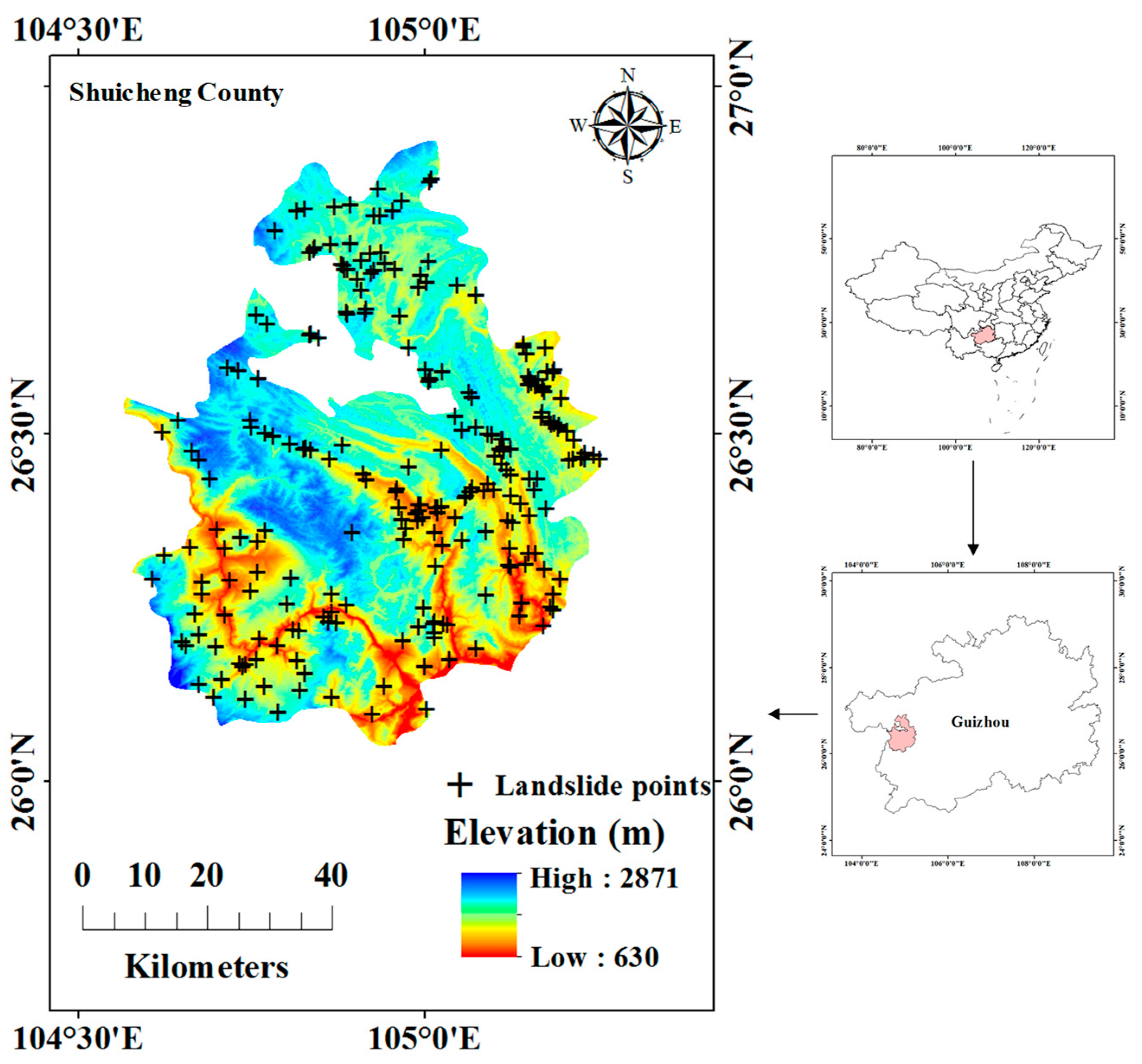
2.1. Study Area
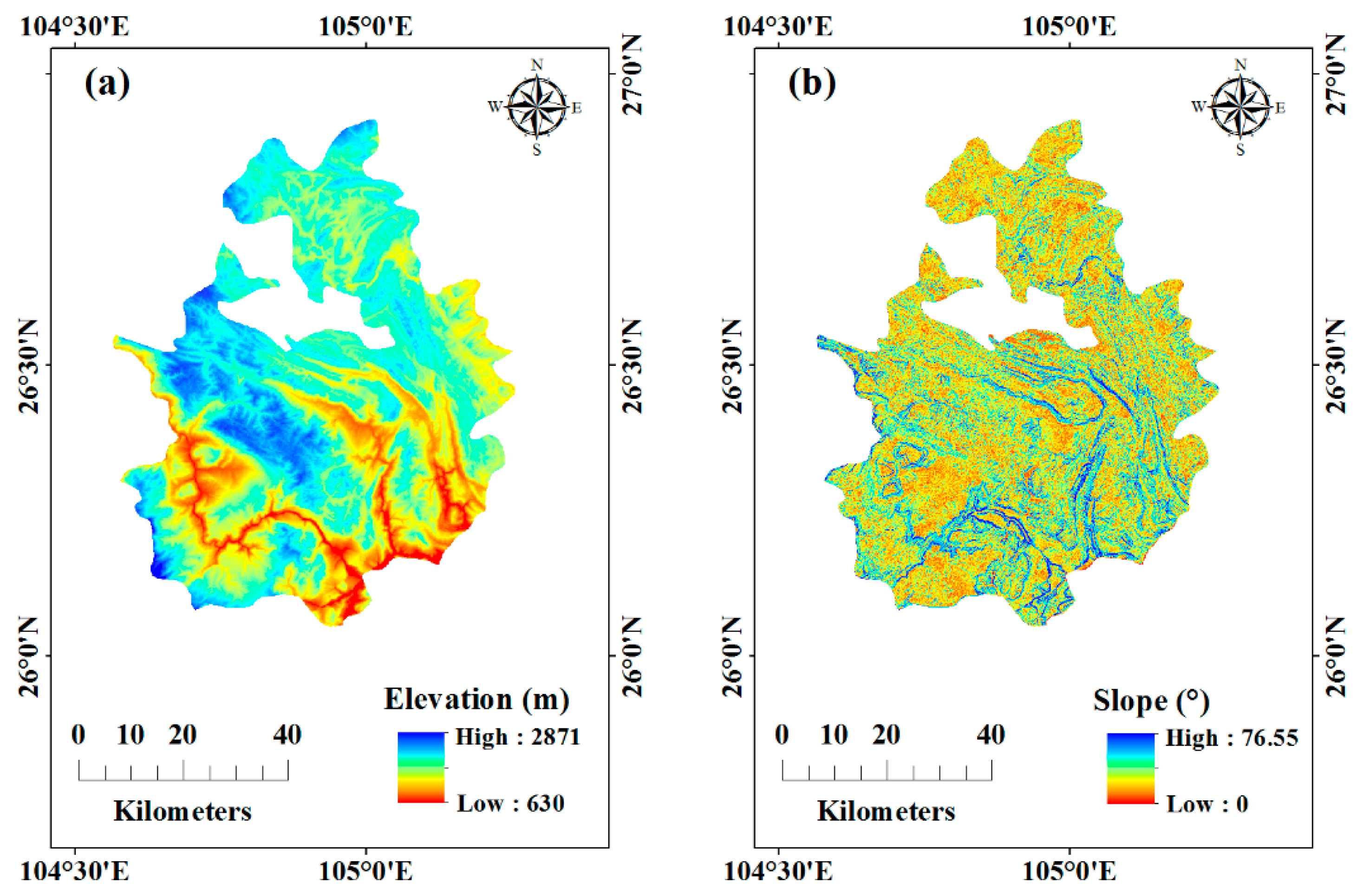
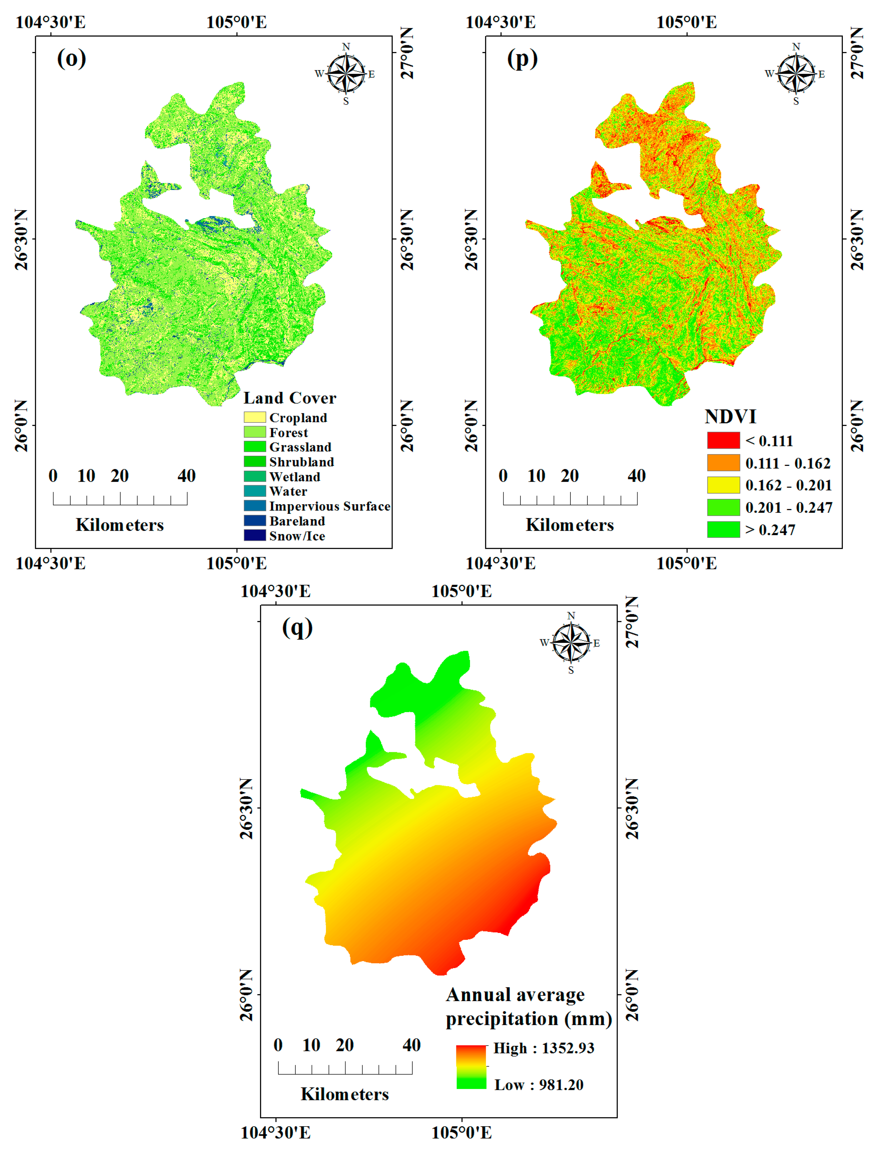
2.2. Data
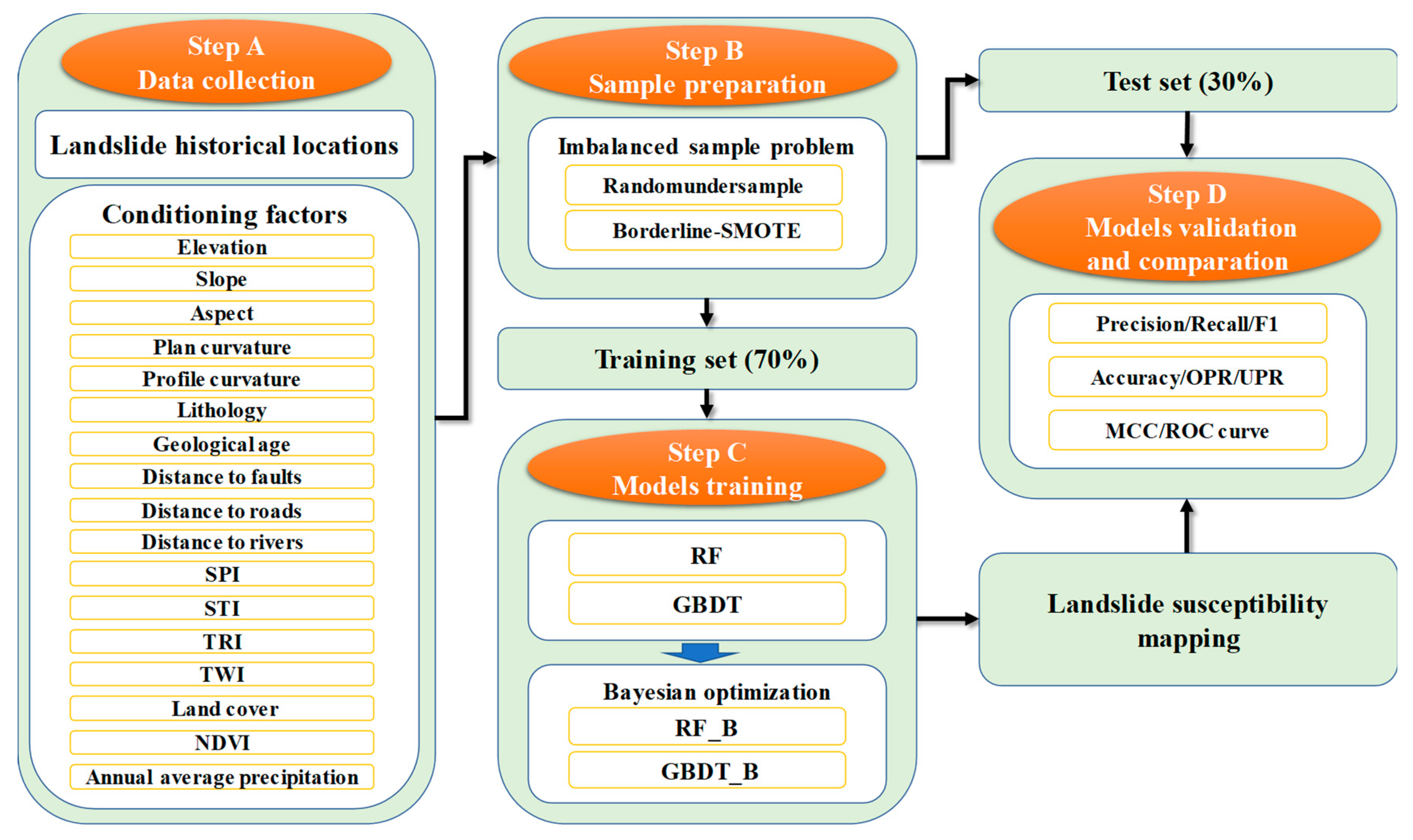
3. Methods
3.1. Data Pretreatment
3.2. Imbalanced Sample Problem and Sample Preparation
3.3. RF Model
3.4. GBDT Model
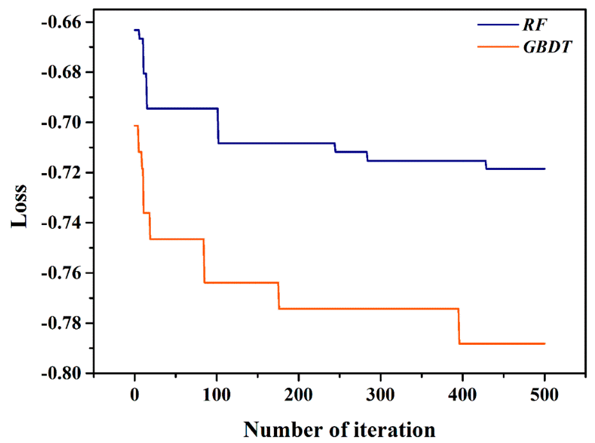
3.5. Bayesian Optimization
3.6. Model Evaluation
4. Results
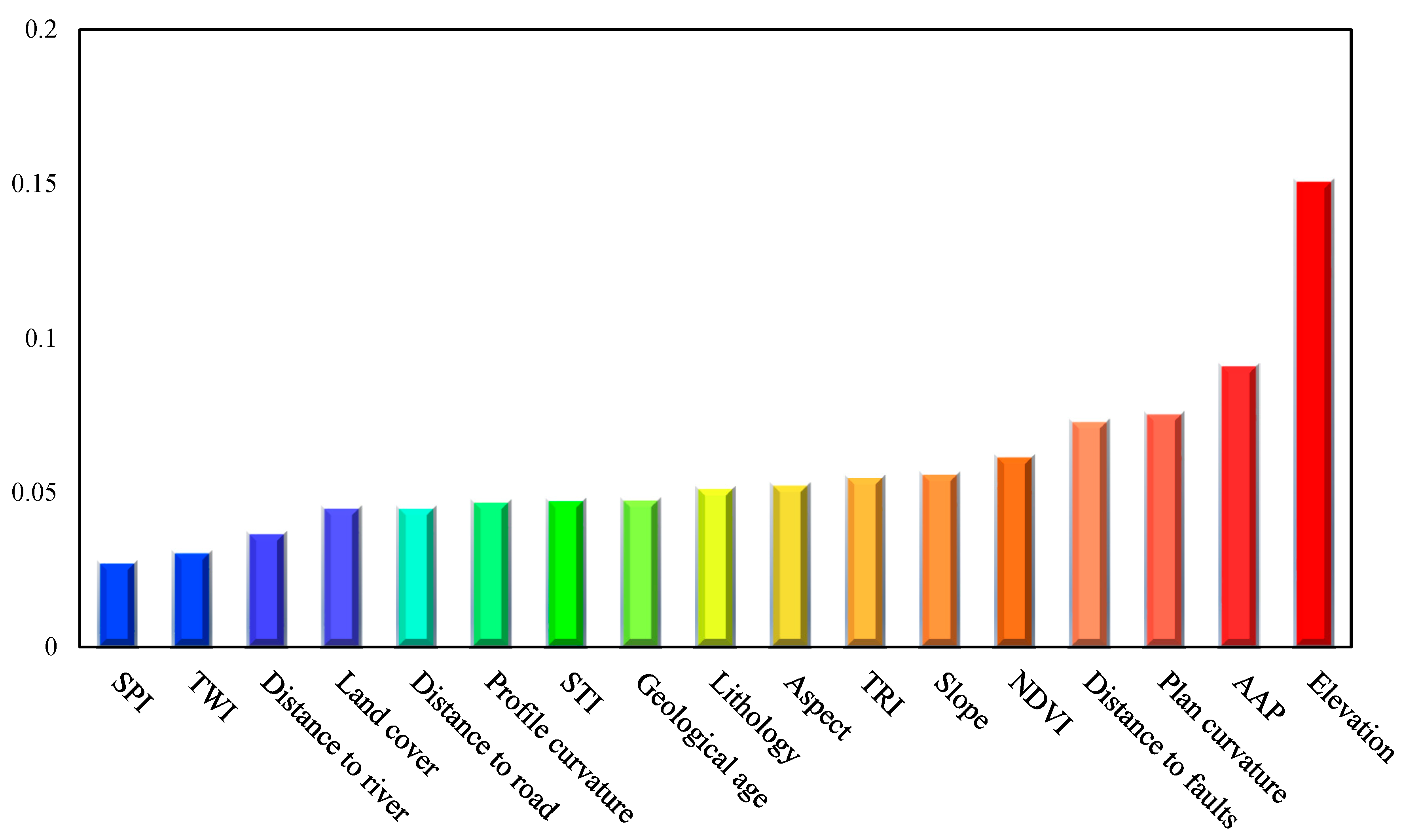
4.1. Feature Importance
4.2. Results of Bayesian Optimization
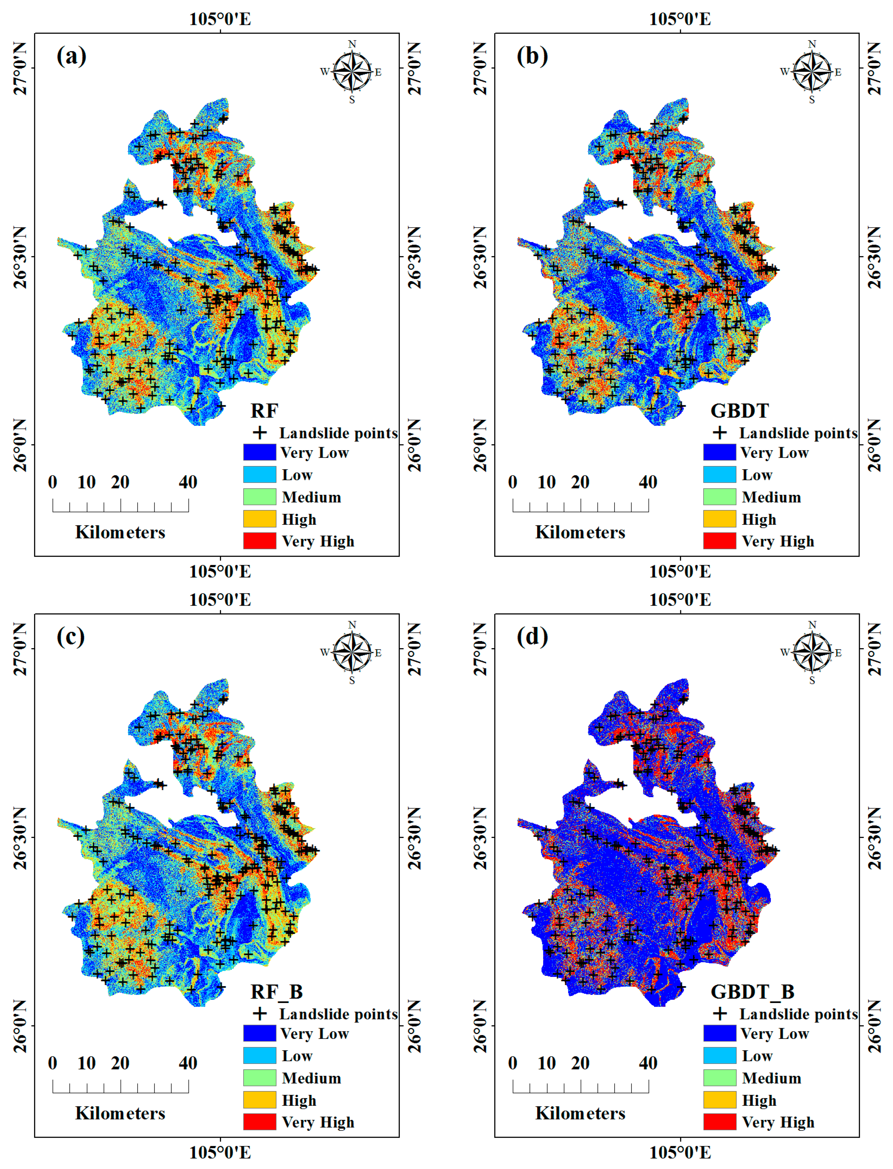
4.3. LSMs Based Multiple Models
4.4. Model Comparison and Validation
5. Discussion
6. Conclusions
Author Contributions
Funding
Acknowledgments
Conflicts of Interest
Data and Code Availability
References
- Zhu, A.; Miao, Y.; Yang, L.; Bai, S.; Liu, J.; Hong, H. Comparison of the presence-only method and presence-absence method in landslide susceptibility mapping. Catena 2018, 171, 222–233. [Google Scholar] [CrossRef]
- Petley, D. Global patterns of loss of life from landslides. Geology 2012, 40, 927–930. [Google Scholar] [CrossRef]
- Gao, J.; Sang, Y. Identification and estimation of landslide-debris flow disaster risk in primary and middle school campuses in a mountainous area of Southwest China. Int. J. Disast. Risk Reduct. 2017, 25, 60–71. [Google Scholar] [CrossRef]
- Haque, U.; Blum, P.; Da Silva, A.P.F.; Andersen, P.; Pilz, J.; Chalov, S.R.; Malet, J.-P.; Auflič, M.J.; Andres, N.; Poyiadji, E.; et al. Fatal landslides in Europe. Landslides 2016, 13, 1545–1554. [Google Scholar] [CrossRef]
- Dai, F.C.; Lee, C.F.; Ngai, Y.Y. Landslide risk assessment and management: An overview. Eng. Geol. 2002, 64, 65–87. [Google Scholar] [CrossRef]
- Golovko, D.; Roessner, S.; Behling, R.; Wetzel, H.-U.; Kleinschmit, B. Evaluation of Remote-Sensing-Based Landslide Inventories for Hazard Assessment in Southern Kyrgyzstan. Remote Sens. 2017, 9, 943. [Google Scholar] [CrossRef] [Green Version]
- Choi, J.; Oh, H.; Lee, H.; Lee, C.; Lee, S. Combining landslide susceptibility maps obtained from frequency ratio, logistic regression, and artificial neural network models using ASTER images and GIS. Eng. Geol. 2012, 124, 12–23. [Google Scholar] [CrossRef]
- Wu, C. Landslide Susceptibility Based on Extreme Rainfall-Induced Landslide Inventories and the Following Landslide Evolution. Water 2019, 11, 2609. [Google Scholar] [CrossRef] [Green Version]
- Han, L.; Zhang, J.; Zhang, Y.; Lang, Q. Applying a Series and Parallel Model and a Bayesian Networks Model to Produce Disaster Chain Susceptibility Maps in the Changbai Mountain area, China. Water 2019, 11, 2144. [Google Scholar] [CrossRef] [Green Version]
- Yi, Y.; Zhang, Z.; Zhang, W.; Xu, Q.; Deng, C.; Li, Q. GIS-based earthquake-triggered-landslide susceptibility mapping with an integrated weighted index model in Jiuzhaigou region of Sichuan Province, China. Nat. Hazards Earth Syst. Sci. 2019, 19, 1973–1988. [Google Scholar] [CrossRef] [Green Version]
- Long, N.; De Smedt, F. Analysis and Mapping of Rainfall-Induced Landslide Susceptibility in A Luoi District, Thua Thien Hue Province, Vietnam. Water 2019, 11, 51. [Google Scholar] [CrossRef] [Green Version]
- Yang, J.; Song, C.; Yang, Y.; Xu, C.; Guo, F.; Xie, L. New method for landslide susceptibility mapping supported by spatial logistic regression and GeoDetector: A case study of Duwen Highway Basin, Sichuan Province, China. Geomorphology 2019, 324, 62–71. [Google Scholar] [CrossRef]
- Pham, B.T.; Bui, D.T.; Pourghasemi, H.R.; Indra, P.; Dholakia, M.B. Landslide susceptibility assesssment in the Uttarakhand area (India) using GIS: A comparison study of prediction capability of naïve bayes, multilayer perceptron neural networks, and functional trees methods. Theor. Appl. Clim. 2017, 128, 255–273. [Google Scholar] [CrossRef]
- Mao, Y.; Zhang, M.; Sun, P.; Wang, G. Landslide susceptibility assessment using uncertain decision tree model in loess areas. Environ. Earth Sci. 2017, 76, 752. [Google Scholar] [CrossRef]
- Aktas, H.; San, B.T. Landslide susceptibility mapping using an automatic sampling algorithm based on two level random sampling. Comput. Geosci. 2019, 133, 104329. [Google Scholar] [CrossRef]
- Huang, Y.; Zhao, L. Review on landslide susceptibility mapping using support vector machines. Catena 2018, 165, 520–529. [Google Scholar] [CrossRef]
- Dou, J.; Chang, K.-T.; Chen, S.; Yunus, A.P.; Liu, J.-K.; Xia, H.; Zhu, Z. Automatic Case-Based Reasoning Approach for Landslide Detection: Integration of Object-Oriented Image Analysis and a Genetic Algorithm. Remote Sens. 2015, 7, 4318–4342. [Google Scholar] [CrossRef] [Green Version]
- Bragagnolo, L.; da Silva, R.; Grzybowski, J. Artificial neural network ensembles applied to the mapping of landslide susceptibility. Catena 2020, 184, 104240. [Google Scholar] [CrossRef]
- Zhou, C.; Yin, K.; Cao, Y.; Ahmed, B.; Li, Y.; Catani, F.; Pourghasemi, H.R. Landslide susceptibility modeling applying machine learning methods: A case study from Longju in the Three Gorges Reservoir Area, China. Comput. Geosci. 2018, 112, 23–37. [Google Scholar] [CrossRef] [Green Version]
- Wang, Y.; Fang, Z.; Hong, H. Comparison of convolutional neural networks for landslide susceptibility mapping in Yanshan County, China. Sci. Total Environ. 2019, 666, 975–993. [Google Scholar] [CrossRef] [PubMed]
- Wang, Y.; Fang, Z.; Wang, M.; Peng, L.; Hong, H. Comparative study of landslide susceptibility mapping with different recurrent neural networks. Comput. Geosci. 2020, 138, 104445. [Google Scholar] [CrossRef]
- Dou, J.; Yunus, A.P.; Bui, D.T.; Merghadi, A.; Sahana, M.; Zhu, Z.; Chen, C.-W.; Khosravi, K.; Yang, Y.; Pham, B.T. Assessment of advanced random forest and decision tree algorithms for modeling rainfall-induced landslide susceptibility in the Izu-Oshima Volcanic Island, Japan. Sci. Total Environ. 2019, 662, 332–346. [Google Scholar] [CrossRef] [PubMed]
- Hong, H.; Miao, Y.; Liu, J.; Zhu, A. Exploring the effects of the design and quantity of absence data on the performance of random forest-based landslide susceptibility mapping. Catena 2019, 176, 45–64. [Google Scholar] [CrossRef]
- Kirschbaum, D.; Stanley, T.; Yatheendradas, S. Modeling landslide susceptibility over large regions with fuzzy overlay. Landslides 2016, 13, 485–496. [Google Scholar] [CrossRef]
- Jebur, M.N.; Pradhan, B.; Tehrany, M.S. Optimization of landslide conditioning factors using very high-resolution airborne laser scanning (LiDAR) data at catchment scale. Remote Sens. Environ. 2014, 152, 150–165. [Google Scholar] [CrossRef]
- Shahri, A.; Spross, J.; Johansson, F.; Larsson, S. Landslide susceptibility hazard map in southwest Sweden using artificial neural network. Catena 2019, 183, 104225. [Google Scholar] [CrossRef]
- Melillo, M.; Brunetti, M.T.; Peruccacci, S.; Gariano, S.L.; Guzzetti, F. An algorithm for the objective reconstruction of rainfall events responsible for landslides. Landslides 2015, 12, 311–320. [Google Scholar] [CrossRef]
- Lee, M.; Ng, K.; Huang, Y.; Li, W. Rainfall-induced landslides in Hulu Kelang area, Malaysia. Nat. Hazards 2014, 70, 353–375. [Google Scholar] [CrossRef]
- Conte, E.; Troncone, A. A method for the analysis of soil slips triggered by rainfall. Géotechnique 2012, 62, 187–192. [Google Scholar] [CrossRef]
- Guzzetti, F.; Peruccacci, S.; Rossi, M.; Stark, C.P. Rainfall thresholds for the initiation of landslides in central and southern Europe. Meteorol. Atmos. Phys. 2007, 98, 239–267. [Google Scholar] [CrossRef]
- Brunetti, M.T.; Peruccacci, S.; Rossi, M.; Luciani, S.; Valigi, D.; Guzzetti, F. Rainfall thresholds for the possible occurrence of landslides in Italy. Nat. Hazards Earth Syst. Sci. 2010, 10, 447–458. [Google Scholar] [CrossRef]
- Conte, E.; Troncone, A. Analytical Method for Predicting the Mobility of Slow-Moving Landslides owing to Groundwater Fluctuations. J. Geotech. Geoenviron. Eng. 2011, 137, 777–784. [Google Scholar] [CrossRef]
- Conte, E.; Troncone, A. Stability analysis of infinite clayey slopes subjected to pore pressure changes. Géotechnique 2012, 62, 87–91. [Google Scholar] [CrossRef]
- Guizhou Provincial Bureau of Statistics. Available online: http://stjj.guizhou.gov.cn (accessed on 16 April 2020).
- Zhao, W.; Wang, R.; Liu, X.; Ju, N.; Xie, M. Field survey of a catastrophic high-speed long-runout landslide in Jichang Town, Shuicheng County, Guizhou, China, on 23 July 2019. Landslides 2020, 17, 1415–1427. [Google Scholar] [CrossRef]
- Rong, G.; Li, K.; Han, L.; Alu, S.; Zhang, J.; Zhang, Y. Hazard Mapping of the Rainfall–Landslides Disaster Chain Based on GeoDetector and Bayesian Network Models in Shuicheng County, China. Water 2020, 12, 2572. [Google Scholar] [CrossRef]
- China Geological Survey. Available online: http://www.cgs.gov.cn (accessed on 16 April 2020).
- Dou, J.; Yunus, A.P.; Merghadi, A.; Shirzadi, A.; Nguyen, H.; Hussain, Y.; Avtar, R.; Chen, Y.; Pham, B.T.; Yamagishi, H. Different sampling strategies for predicting landslide susceptibilities are deemed less consequential with deep learning. Sci. Total Environ. 2020, 720, 137320. [Google Scholar] [CrossRef]
- Du, G.; Zhang, Y.; Iqbal, J.; Yang, Z.; Yao, X. Landslide susceptibility mapping using an integrated model of information value method and logistic regression in the Bailongjiang watershed, Gansu Province, China. J. Mt. Sci. 2017, 14, 249–268. [Google Scholar] [CrossRef]
- Chinese Academy of Sciences. Geospatial Data Cloud Site. Available online: http://www.gscloud.cn (accessed on 21 March 2020).
- Aghdam, I.; Pradhan, B.; Panahi, M. Landslide susceptibility assessment using a novel hybrid model of statistical bivariate methods (FR and WOE) and adaptive neuro-fuzzy inference system (ANFIS) at southern Zagros Mountains in Iran. Environ. Earth Sci. 2017, 76, 237. [Google Scholar] [CrossRef]
- Sameen, M.I.; Pradhan, B.; Lee, S. Application of convolutional neural networks featuring Bayesian optimization for landslide susceptibility assessment. Catena 2020, 186, 104249. [Google Scholar] [CrossRef]
- Abdollahi, S.; Pourghasemi, H.; Ghanbarian, G.; Safaeian, R. Prioritization of effective factors in the occurrence of land subsidence and its susceptibility mapping using an SVM model and their different kernel functions. Bull. Eng. Geol. Environ. 2019, 78, 4017–4034. [Google Scholar] [CrossRef]
- Regmi, N.; Giardino, J.; Vitek, J. Modeling susceptibility to landslides using the weight of evidence approach: Western Colorado, USA. Geomorphology 2010, 115, 172–187. [Google Scholar] [CrossRef]
- Pham, B.T.; Bui, D.T.; Prakash, I.; Dholakia, M.B. Rotation forest fuzzy rule-based classifier ensemble for spatial prediction of landslides using GIS. Nat. Hazards 2016, 83, 97–127. [Google Scholar] [CrossRef]
- Tong, S.; Zhang, J.; Ha, S.; Lai, Q.; Ma, Q. Dynamics of Fractional Vegetation Coverage and Its Relationship with Climate and Human Activities in Inner Mongolia, China. Remote Sens. 2016, 8, 776. [Google Scholar] [CrossRef] [Green Version]
- Finer Resolution Observation and Monitoring of Global Land Cover. Available online: https://data.ess.tsinghua.edu.cn (accessed on 16 April 2020).
- U.S. Geological Survey. Available online: https://earthexplorer.usgs.gov (accessed on 31 August 2019).
- China Meteorological Data Service Center. Available online: https://data.cma.cn (accessed on 31 August 2019).
- Zhang, Y.; Ge, T.; Tian, W.; Liou, Y. Debris Flow Susceptibility Mapping Using Machine-Learning Techniques in Shigatse Area, China. Remote Sens. 2019, 11, 2801. [Google Scholar] [CrossRef] [Green Version]
- Song, Y.; Niu, R.; Xu, S.; Ye, R.; Peng, L.; Guo, T.; Li, S.; Chen, T. Landslide Susceptibility Mapping Based on Weighted Gradient Boosting Decision Tree in Wanzhou Section of the Three Gorges Reservoir Area, China. ISPRS Int. J. Geo-Inf. 2019, 8, 4. [Google Scholar] [CrossRef] [Green Version]
- Breiman, L. Random forests. Mach. Learn. 2001, 45, 5–32. [Google Scholar] [CrossRef] [Green Version]
- Friedman, J. Greedy function approximation: A gradient boosting machine. Ann. Stat. 2001, 29, 1189–1232. [Google Scholar] [CrossRef]
- Brown, I.; Mues, C. An experimental comparison of classification algorithms for imbalanced credit scoring data sets. Expert Syst. Appl. 2012, 39, 3446–3453. [Google Scholar] [CrossRef] [Green Version]
- Sameen, M.; Pradhan, B.; Lee, S. Self-Learning Random Forests Model for Mapping Groundwater Yield in Data-Scarce Areas. Nat. Resour. Res. 2019, 28, 757–775. [Google Scholar] [CrossRef]
- Shen, X.; Cao, L. Tree-Species Classification in Subtropical Forests Using Airborne Hyperspectral and LiDAR Data. Remote Sens. 2017, 9, 1180. [Google Scholar] [CrossRef] [Green Version]
- Li, Y.; Xia, J.; Zhang, S.; Yan, J.; Ai, X.; Dai, K. An efficient intrusion detection system based on support vector machines and gradually feature removal method. Expert Syst. Appl. 2012, 39, 424–430. [Google Scholar] [CrossRef]
- Fawcett, T. An introduction to ROC analysis. Pattern Recogn. Lett. 2006, 27, 861–874. [Google Scholar] [CrossRef]
- Nhu, V.; Hoang, N.; Nguyen, H.; Ngo, P.; Bui, T.; Hoa, P.; Samui, P.; Bui, D. Effectiveness assessment of Keras based deep learning with different robust optimization algorithms for shallow landslide susceptibility mapping at tropical area. Catena 2020, 188, 104458. [Google Scholar] [CrossRef]
- Alatorre, L.; Sanchez-Andres, R.; Cirujano, S.; Begueria, S.; Sanchez-Carrillo, S. Identification of Mangrove Areas by Remote Sensing: The ROC Curve Technique Applied to the Northwestern Mexico Coastal Zone Using Landsat Imagery. Remote Sens. 2011, 3, 1568–1583. [Google Scholar] [CrossRef] [Green Version]
- Tsangaratos, P.; Ilia, I.; Hong, H.; Chen, W.; Xu, C. Applying Information Theory and GIS-based quantitative methods to produce landslide susceptibility maps in Nancheng County, China. Landslides 2017, 14, 1091–1111. [Google Scholar] [CrossRef]
- Sun, D.; Wen, H.; Wang, D.; Xu, J. A random forest model of landslide susceptibility mapping based on hyperparameter optimization using Bayes algorithm. Geomorphology 2020, 362, 107201. [Google Scholar] [CrossRef]
- Esper Angillieri, M.Y. Debris flow susceptibility mapping using frequency ratio and seed cells, in a portion of a mountain international route, Dry Central Andes of Argentina. Catena 2020, 189, 104504. [Google Scholar] [CrossRef]
- Bui, D.T.; Tsangaratos, P.; Nguyen, V.; Liem, N.V.; Trinh, P.T. Comparing the prediction performance of a Deep Learning Neural Network model with conventional machine learning models in landslide susceptibility assessment. Catena 2020, 188, 104426. [Google Scholar] [CrossRef]
- Huang, F.; Cao, Z.; Guo, J.; Jiang, S.; Li, S.; Guo, Z. Comparisons of heuristic, general statistical and machine learning models for landslide susceptibility prediction and mapping. Catena 2020, 191, 104580. [Google Scholar] [CrossRef]
- Kim, J.; Lee, S.; Jung, H.; Lee, S. Landslide susceptibility mapping using random forest and boosted tree models in Pyeong-Chang, Korea. Geocarto Int. 2018, 33, 1000–1015. [Google Scholar] [CrossRef]
- Chen, W.; Sun, Z.; Han, J. Landslide Susceptibility Modeling Using Integrated Ensemble Weights of Evidence with Logistic Regression and Random Forest Models. Appl. Sci. 2019, 9, 171. [Google Scholar] [CrossRef] [Green Version]


| Conditioning Factor | Data Structure | Data Summary |
|---|---|---|
| Elevation | Raster | Height above sea level |
| Slope | Raster | Calculated by DEM |
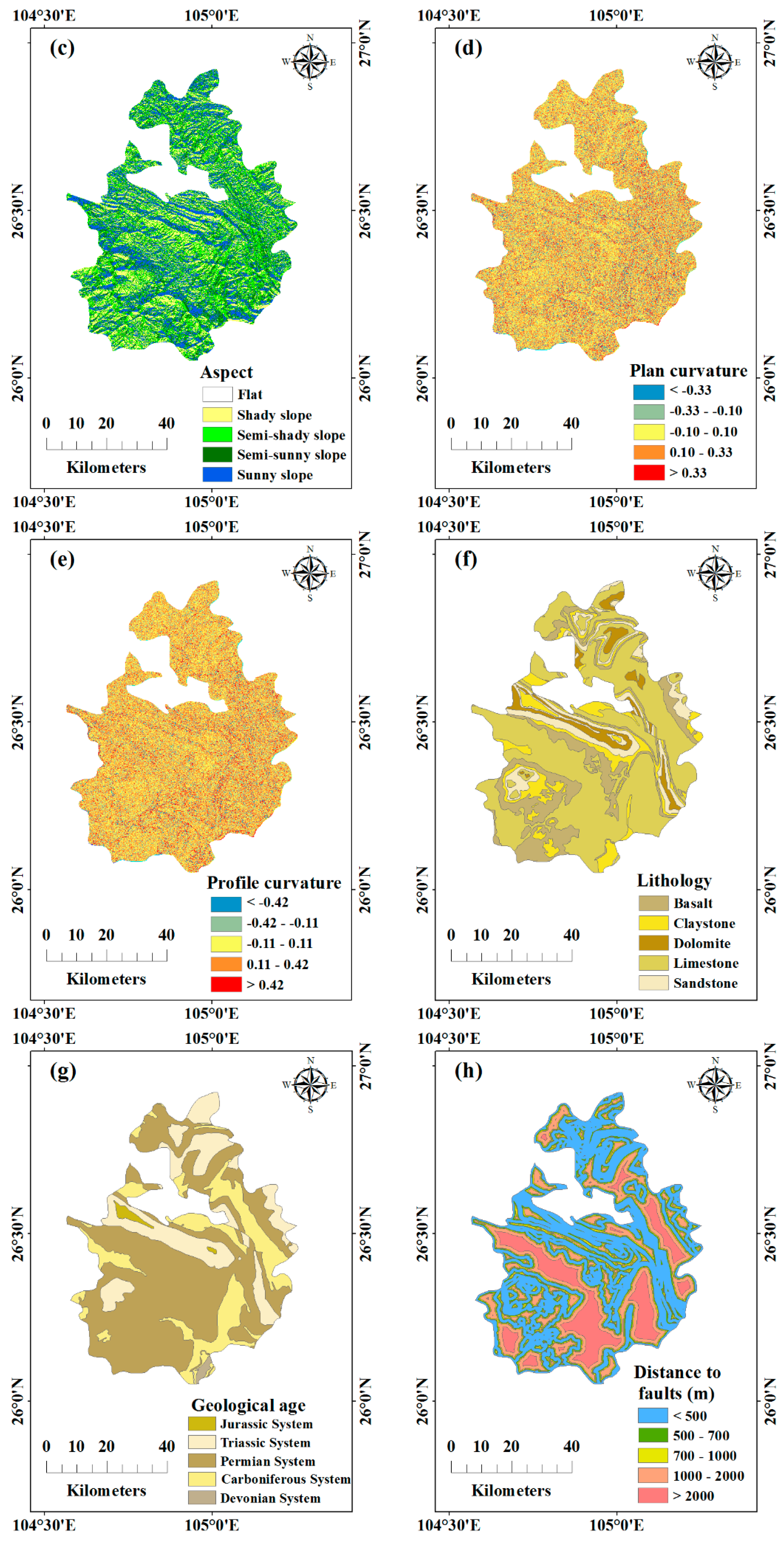
| Aspect | Raster | Calculated by DEM |
| Plan curvature | Raster | Calculated by DEM |
| Profile curvature | Raster | Calculated by DEM |
| Lithology | Polygon | Digitized from lithology map |
| Geological age | Polygon | Digitized from geological age map |
| Faults | Line | Distance to faults |
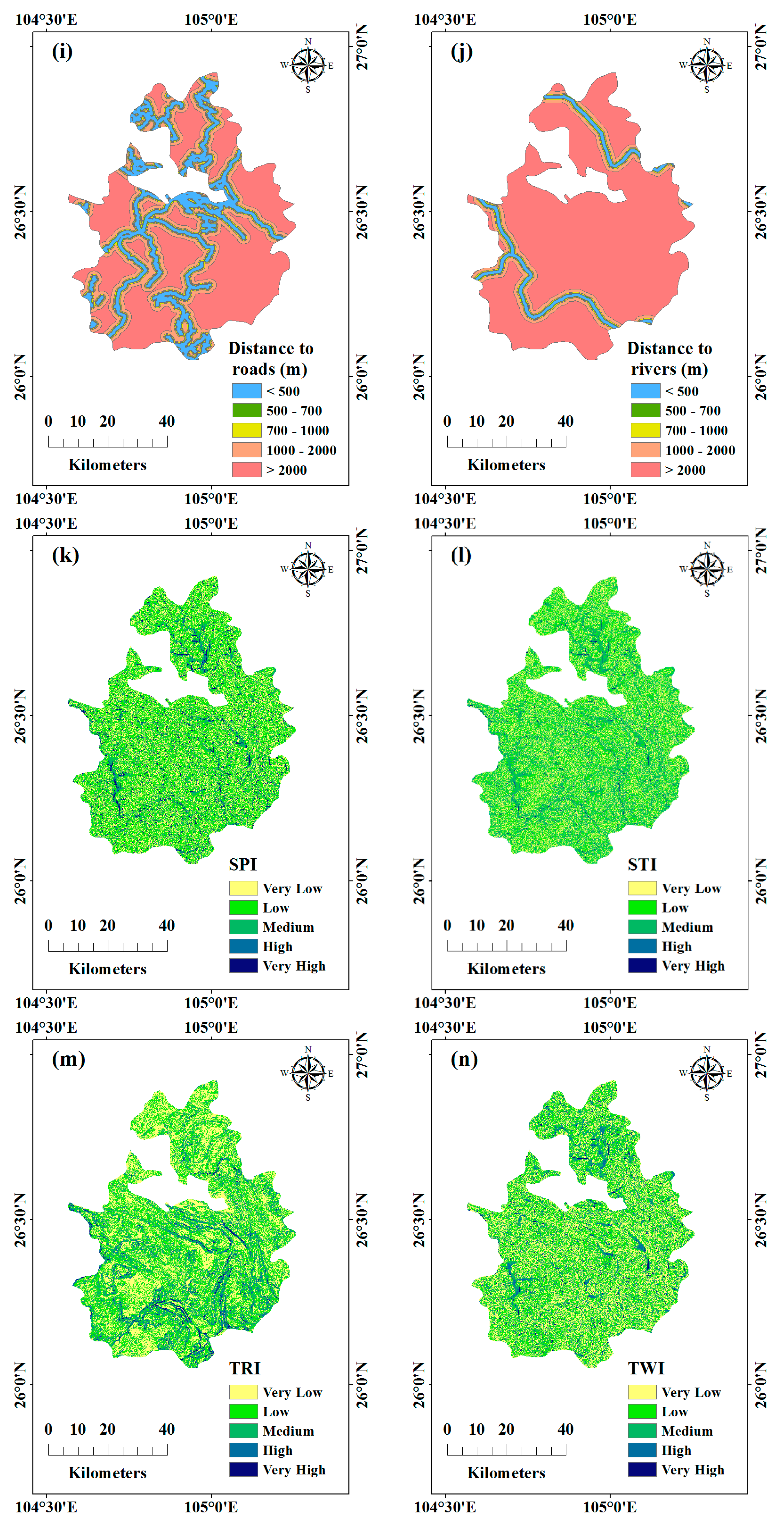
| Roads | Line | Distance to roads |
| Rivers | Line | Distance to rivers |
| SPI | Raster | Calculated by DEM |
| STI | Raster | Calculated by DEM |
| TRI | Raster | Calculated by DEM |
| TWI | Raster | Calculated by DEM |
| Land cover | Raster | The category of land cover |
| NDVI | Raster | The Vegetation cover index |
| Precipitation | Raster | Annual average precipitation |
| Model | Hyperparameter | Default Value | Search Space |
|---|---|---|---|
| RF | N_Estimators | 100 | (50, 500) |
| Max_Depth | None | (1, 100) | |
| Min_Sample_Leaf | 1 | (1, 100) | |
| Max_Leaf_Nodes | Max Value (factor number) | (2, 17) | |
| GBDT | N_Estimators | 100 | (50, 500) |
| Max_Depth | None | (1, 100) | |
| Min_Sample_Leaf | 1 | (1, 100) | |
| Max_Leaf_Nodes | Max Value (factor number) | (2, 17) | |
| Learning_Rate | 1.0 | (0.1, 1.0) | |
| Subsample | 1.0 | (0.5, 1.0) |
| Model | Hyperparameter | Bayesian Optimization Result |
|---|---|---|
| RF | N_Estimators | 252 |
| Max_Depth | 42 | |
| Min_Sample_Leaf | 1 | |
| Max_Leaf_Nodes | 17 | |
| GBDT | N_Estimators | 310 |
| Max_Depth | 47 | |
| Min_Sample_Leaf | 2 | |
| Max_Leaf_Nodes | 17 | |
| Learning_Rate | 0.30346 | |
| Subsample | 0.95475 |
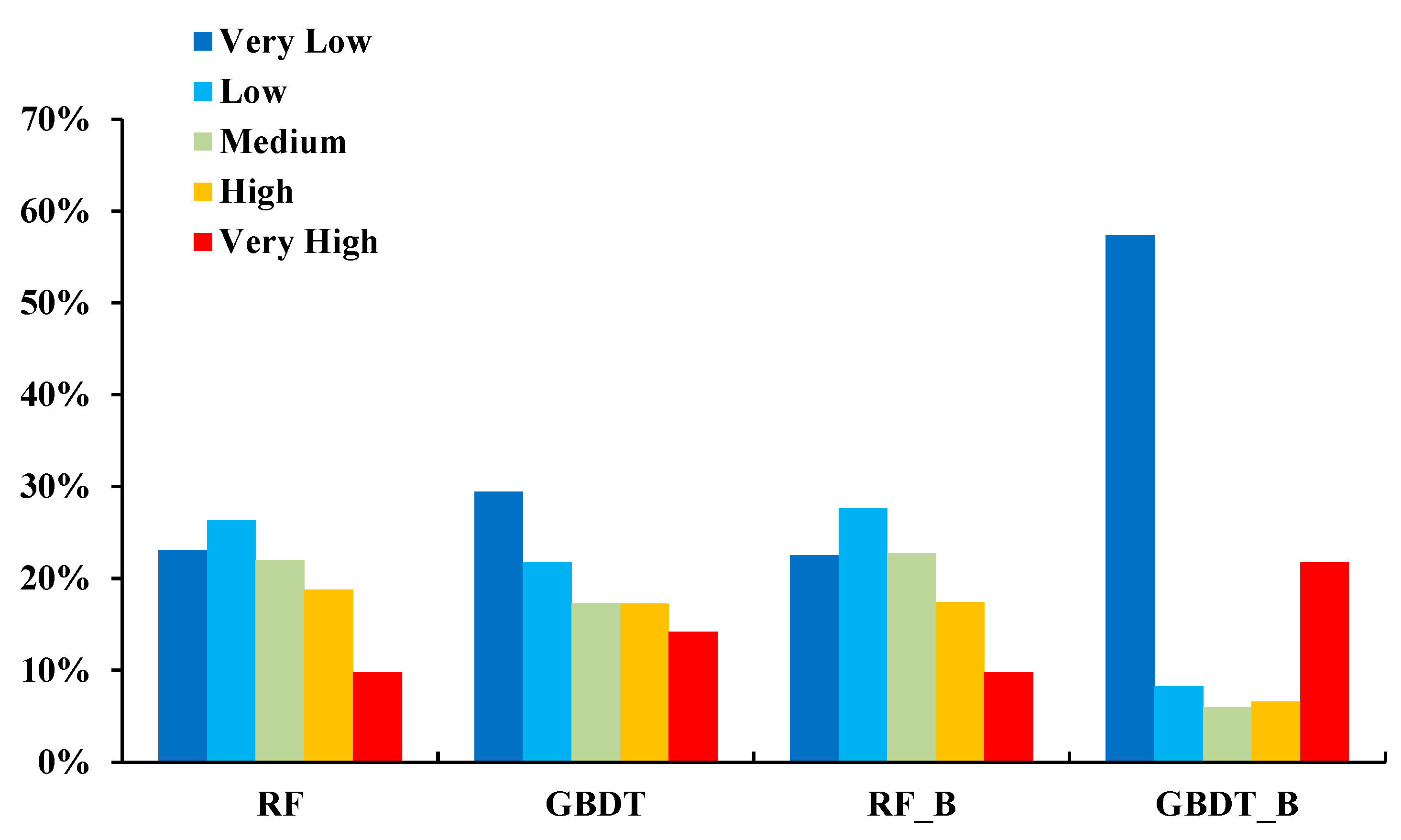
| RF | GBDT | RF_B | GBDT_B | |||||
|---|---|---|---|---|---|---|---|---|
| LSM Grade | Count | Pli (%) | Count | Pli (%) | Count | Pli (%) | Count | Pli (%) |
| Very Low | 7 | 2.92 | 21 | 8.75 | 8 | 3.33 | 17 | 7.08 |
| Low | 31 | 12.92 | 19 | 7.92 | 33 | 13.75 | 7 | 2.92 |
| Medium | 50 | 20.83 | 34 | 14.12 | 49 | 20.42 | 5 | 2.08 |
| High | 85 | 35.42 | 62 | 25.84 | 77 | 32.08 | 12 | 5.00 |
| Very High | 67 | 27.93 | 94 | 39.17 | 73 | 30.42 | 199 | 82.92 |
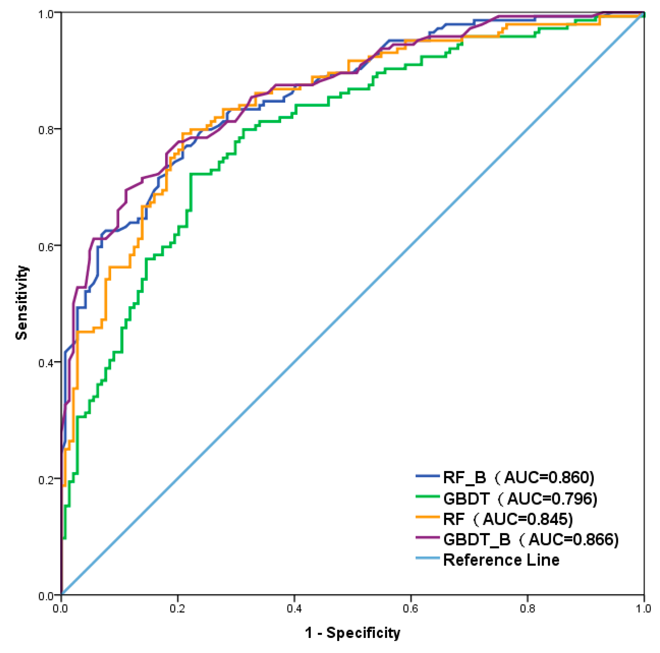
| Model | Test Data Set | Validation Methods | Results | |
|---|---|---|---|---|
| RF | TP | 116 | Precision | 0.739 |
| Recall | 0.806 | |||
| TN | 103 | F1 | 0.771 | |
| Accuracy | 0.760 | |||
| FP | 41 | OPR | 0.261 | |
| UPR | 0.194 | |||
| FN | 28 | MCC | 0.523 | |
| AUC | 0.845 | |||
| GBDT | TP | 116 | Precision | 0.707 |
| Recall | 0.806 | |||
| TN | 96 | F1 | 0.753 | |
| Accuracy | 0.736 | |||
| FP | 48 | OPR | 0.293 | |
| UPR | 0.194 | |||
| FN | 28 | MCC | 0.477 | |
| AUC | 0.796 | |||
| RF_B | TP | 119 | Precision | 0.744 |
| Recall | 0.826 | |||
| TN | 103 | F1 | 0.783 | |
| Accuracy | 0.771 | |||
| FP | 41 | OPR | 0.256 | |
| UPR | 0.174 | |||
| FN | 25 | MCC | 0.545 | |
| AUC | 0.860 | |||
| GBDT_B | TP | 115 | Precision | 0.782 |
| Recall | 0.799 | |||
| TN | 112 | F1 | 0.790 | |
| Accuracy | 0.788 | |||
| FP | 32 | OPR | 0.218 | |
| UPR | 0.201 | |||
| FN | 29 | MCC | 0.576 | |
| AUC | 0.866 | |||
Publisher’s Note: MDPI stays neutral with regard to jurisdictional claims in published maps and institutional affiliations. |
© 2020 by the authors. Licensee MDPI, Basel, Switzerland. This article is an open access article distributed under the terms and conditions of the Creative Commons Attribution (CC BY) license (http://creativecommons.org/licenses/by/4.0/).
Share and Cite
Rong, G.; Alu, S.; Li, K.; Su, Y.; Zhang, J.; Zhang, Y.; Li, T. Rainfall Induced Landslide Susceptibility Mapping Based on Bayesian Optimized Random Forest and Gradient Boosting Decision Tree Models—A Case Study of Shuicheng County, China. Water 2020, 12, 3066. https://doi.org/10.3390/w12113066
Rong G, Alu S, Li K, Su Y, Zhang J, Zhang Y, Li T. Rainfall Induced Landslide Susceptibility Mapping Based on Bayesian Optimized Random Forest and Gradient Boosting Decision Tree Models—A Case Study of Shuicheng County, China. Water. 2020; 12(11):3066. https://doi.org/10.3390/w12113066
Chicago/Turabian StyleRong, Guangzhi, Si Alu, Kaiwei Li, Yulin Su, Jiquan Zhang, Yichen Zhang, and Tiantao Li. 2020. "Rainfall Induced Landslide Susceptibility Mapping Based on Bayesian Optimized Random Forest and Gradient Boosting Decision Tree Models—A Case Study of Shuicheng County, China" Water 12, no. 11: 3066. https://doi.org/10.3390/w12113066