Application of Multi-Source Data Fusion Method in Updating Topography and Estimating Sedimentation of the Reservoir


1
School of Hydraulic Engineering, Dalian University of Technology, Dalian 116024, China
2
Department of Geography and Philosophy, University of Minnesota-Duluth, Duluth, MN 55812, USA
*
Author to whom correspondence should be addressed.
Water 2020, 12(11), 3057; https://doi.org/10.3390/w12113057
Submission received: 5 September 2020
/
Revised: 21 October 2020
/
Accepted: 26 October 2020
/
Published: 30 October 2020
(This article belongs to the Special Issue Tools for Water Resources Monitoring, Water Erosion and Geomorphological Research)
Abstract
:The underwater terrain of a reservoir can experience significant changes due to the effects of erosion and siltation during decades of operation. Therefore, existing topographic data no longer reflect current reservoir terrains and need to be updated. In this paper, we propose a fast and economical method for updating the topography of a reservoir. According to multi-source data fusion, we effectively integrated sonar sounding data, cartographic data, and manual measurement data to update and reconstruct the bottom topography of a reservoir in Northeast China. By comparing the updated topography with the measured elevation, the average error of the simulation results is only 0.56%, which shows that the updated topography can accurately reflect the actual topography of the reservoir. Furthermore, by using the surface volume tool in ArcGIS, we developed the original and updated the elevation and volume curves of the reservoir. Finally, the amount of silting and its distribution in the reservoir were obtained by calculating the difference between the original and updated elevation and volume curves. The results show that the total sedimentation volume in the researching reservoir is about 4.3 million m3, which is mainly concentrated in the areas with an elevation below 50 m and above 60 m.
1. Introduction
With the development of economies, the proportion of reservoirs as the main water source of urban water supply is increasing day-by-day [1]. Because pollutants brought into a reservoir by a river are blocked by the reservoir dam, they accumulate in the reservoir and form a potential safety hazard [2,3,4]. Studies on internal pollution sources in a reservoir, including sedimentation, as well as hydrodynamic and water quality simulation, require accurate reservoir topography. However, the underwater terrain of a reservoir keeps changing under the effects of erosion and siltation [5,6,7]. Therefore, to meet the needs of reservoir flood control dispatching and safe operation, timely updating of the topographic data is needed.
The traditional method of underwater measurement consists of establishing a control network, selecting the control section, measuring water depth, and deducing the elevation of reservoir bottom which is difficult to implement and has poor performance in accuracy [8]. Therefore, generally, measurement of reservoir topography, using the traditional method, is only conducted after the reservoir topography has undergone drastic changes. Due to the development of multi-beam underwater sounding methods, bathymetric equipment can achieve full coverage measurement [9]. The combined application of real-time kinetic wave positioning and a bathymeter in a mobile base station network can effectively reduce the errors caused by ship swaying while surveying [10,11]. These advances have greatly improved measurement accuracy, but large-scale underwater measurement still has disadvantages which include huge workload and high cost. Recently, new methods, such as remote sensing measurement and three-dimensional laser scanning, can quickly acquire large-area topographic data and effectively improve the efficiency of surveying and mapping [12,13,14]. However, these methods are either very time-consuming or the accuracy is vulnerable to environmental conditions. Moreover, all of these new methods have expensive drawbacks [15].
In contrast, obtaining the reservoir topography by fusing terrain data of different periods and sources has the advantages of low cost and short cycle [16,17]. Using this method, it is possible to update reservoir terrain with the latest topographic data at any time, which has important practical significance for the operation and management of a reservoir. The research on multi-source terrain data fusion has mainly been based on the improvement and comprehensive application of methods such as tension spline interpolation, kriging interpolation, among others [18,19,20]. For example, Arndt et al. [21] combined multi-source ship sounding data to obtain Antarctic underwater terrain. Miao et al. [22] used the split-sample method to evaluate the uncertainty of multi-source fusion results and constructed a reliable offshore seabed topography. However, the previous research on multi-source terrain data fusion has focused more on the oceans, and much less on reservoirs.
Therefore, based on the analysis of the topographic data characteristics of the reservoir area, in this paper, we propose a data fusion method using multi-source data, including an original topographic map from before construction of a reservoir, a survey map of the reservoir monitoring ship, and scattered direct observation data. Taking a reservoir in Northeast China as an example, first, this method is applied to update the topographic map of the reservoir area; then, the accuracy of the fusion method is evaluated; and the changing volume of erosion and deposition of the reservoir is finally calculated, which will provide practical guidance for managing the reservoir.
2. Study Area and Data Sources
2.1. Study Area and Background
The studied reservoir is located in Dalian. China, which is the water supply source for the city of Dalian (Figure 1). The topographic data of the reservoir was measured before the establishment of the reservoir, in 1984. It has been over 30 years since the reservoir was put into operation, but the topographic data of the reservoir area have never been updated. During this period, due to sedimentation and flooding, the topography of the reservoir area has changed dramatically. Timely updating the topographic data has become an urgent task for ensuring safe operation of the reservoir.
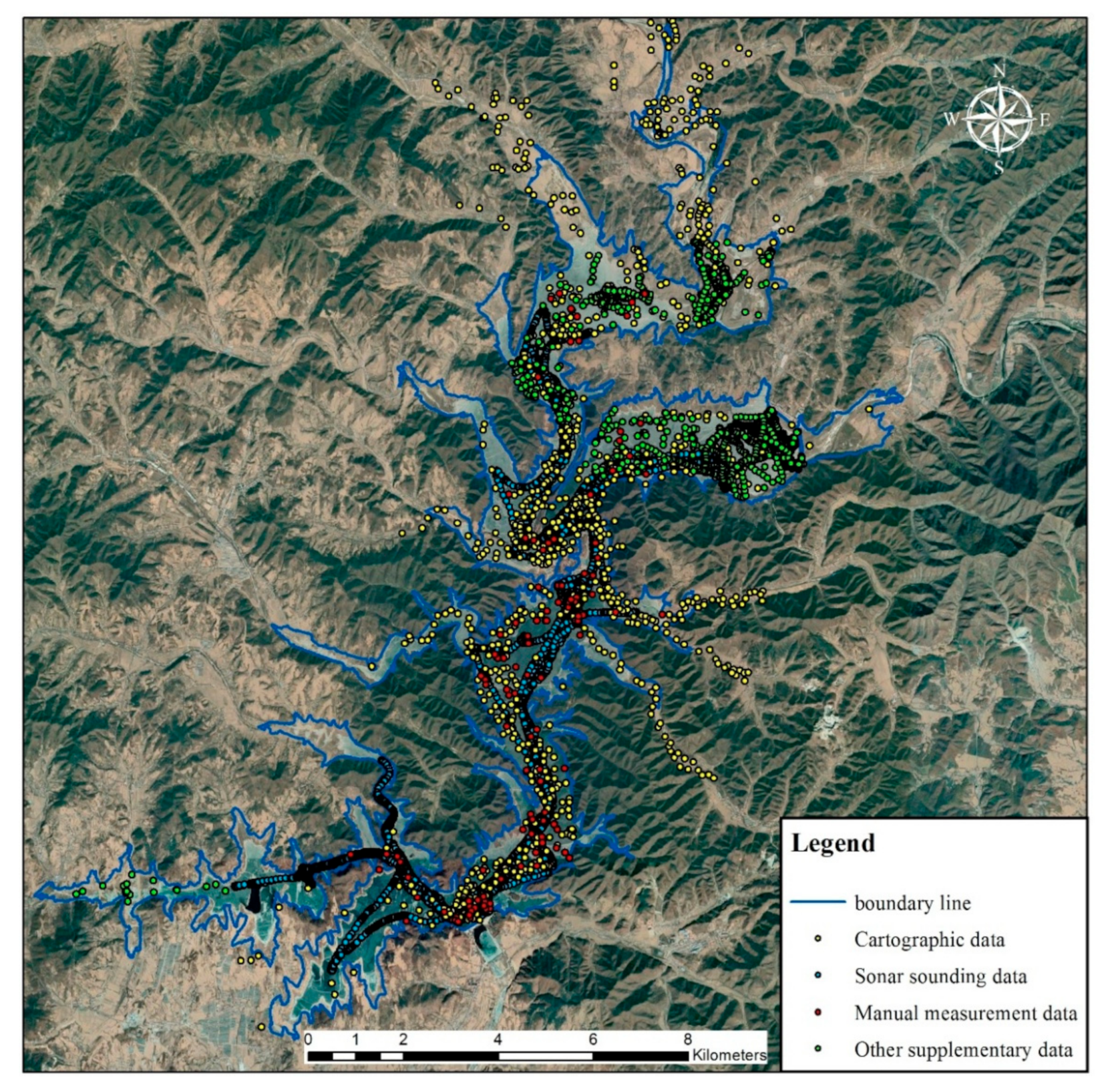
2.2. Data Source and Distribution
The existing topographic data of the reservoir include the following types:
Cartographic data A topographic map was produced in 1958, prior to the reservoir construction, at a scale of 1:5000 with 998 elevation points. This map shows the general topographic characteristics of the area but has deficiencies in accuracy due to the low density of elevation points.
Sonar sounding data The sonar sounding data were measured by a sonar depth sounder installed on the water quality monitoring vessel of the Reservoir Management Bureau, from 2013 to 2015. There were over 9000 track points, mainly distributed on the ship’s routes, with high sampling density and accuracy.
Manual measurement data The manual measurement data were recorded by the Reservoir Management Bureau mainly along the main water quality monitoring section of the reservoir, from 2014 to 2016.
Other supplementary data The supplementary topographic data were measured in the backwater area during the dry season of the reservoir, in 2017.
Figure 2 shows the distribution of multi-source data.
3. Multi-Source Data Fusion Method
The topographic data of different sources vary widely in data accuracy, sampling point density, and data timeliness. Therefore, data fusion needs to be performed first. Previous studies on multi-source terrain data fusion have mainly focused on the ocean. Seabed topography is stable over a long time, which means that there is no time-effect obstacle in the fusion of multi-source data. However, with regard to reservoirs, siltation occurs due to a decrease in the sediment carrying capacity of water flow caused by the slowdown of incoming river flows and the interception effect of dams. Therefore, since the establishment of the reservoir, the topography keeps changing and may change significantly in a short time if extreme hydrological events such as floods occur [23,24]. Accordingly, attention should be paid to the timeliness of data, and the differences in both accuracy and time of data sources should be taken into account when applying the multi-source data fusion in the reservoir.
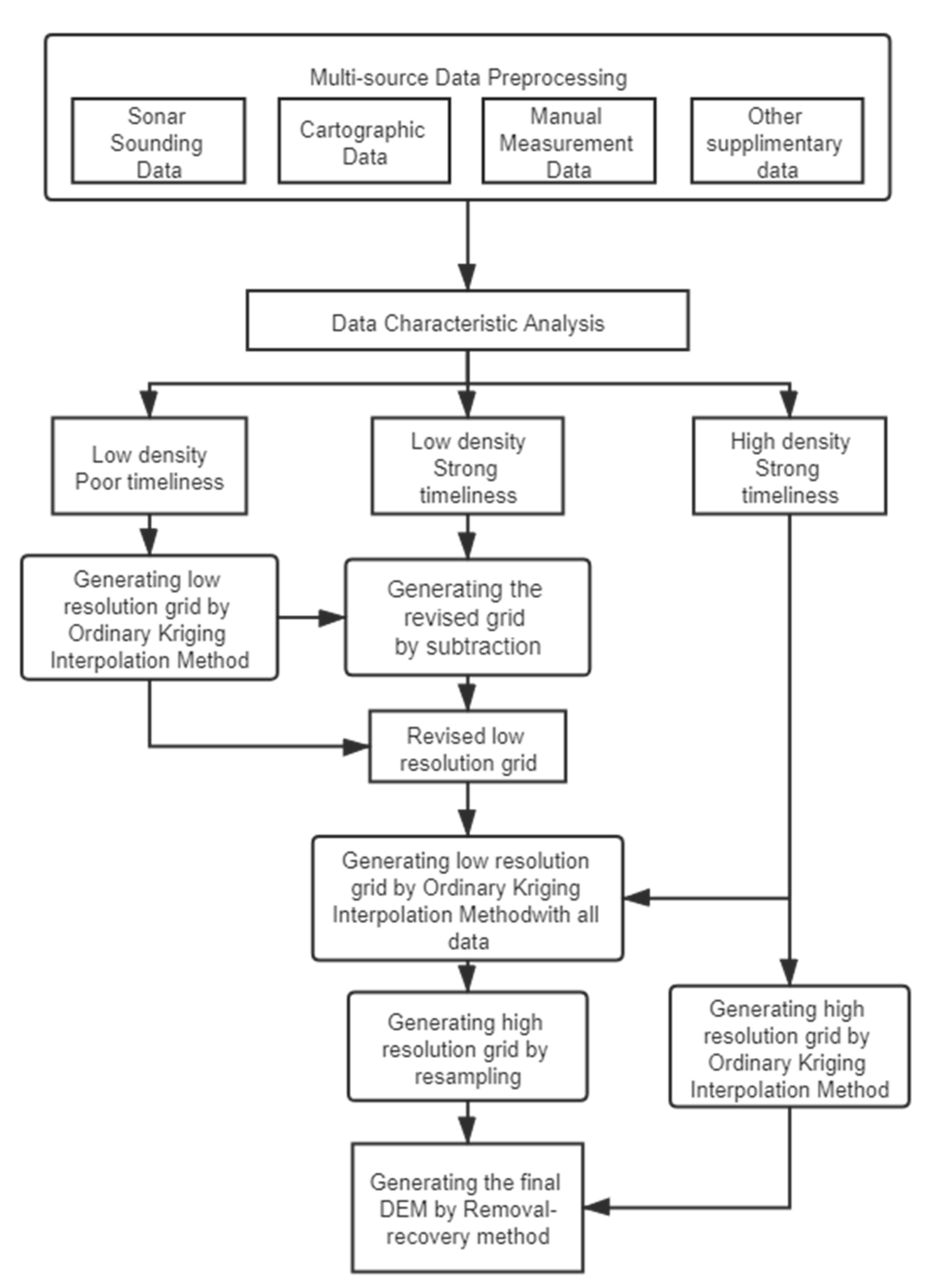
In this paper, we present an appropriate method of multi-source terrain data fusion for reservoirs (Figure 3). The procedures are as follows:
- Unify the format and coordinate system of topographic maps, sonar detection data, and observation points before data fusion.
- Analyze the point density, timeliness, coverage, and other index characteristics of each set of data, then sort and classify the source data according to the density and time.
- Use the difference method to correct or reduce the accuracy errors caused by different acquisition times for the data with similar sampling density [25].
- Use the ordinary kriging interpolation method based on the spherical semi-variogram model to obtain the integrated terrain of the reservoir area.
3.1. Data Preprocessing
Since there are many differences between multi-source data, similar to acquisition, the time of sampling, the format of preservation, and so on, data preprocessing should be taken as follows: (1) using scanning equipment and AutoCAD to computerize the pre-database mapping and correct the errors caused by the drawing deformation; (2) transforming the coordinate system of the digital map to the China Geodetic Coordinate System (CGCS) 1980 through the georeferenced alignment; (3) converting the ship surveyed data and manual data from the geodetic coordinate to CGCS 1980, to achieve the unification of multi-source terrain data with respect to format and coordinate system.
3.2. Data Characteristic Analysis
By comparing the accuracy and coverage of multi-source data, we found:
- Sonar sounding data has a high accuracy of water depth and high density of mining points, but its coverage is narrow, mainly concentrated in the deep-water area from the reservoir center to the front of the dam.
- The elevation points of the topographic map data are sparsely distributed and have a lower accuracy, but almost cover the whole reservoir area.
The amount of direct observation data is limited and mainly distributes in the shallow water area near the upstream river inlet. In terms of data acquisition time, sonar sounding water depth data and direct observation data were newer data that had been collected in recent years, while the topographic mapping data were acquired prior to reservoir construction. While merging multi-source data, data with different coverage complement each other, but those with different timeliness or density interfere with each other and affect the accuracy of the result. According to the data density and timeliness, the reservoir multi-source topographic or water depth data are classified into three categories:
- Data with low-density points and poor timeliness, such as the topographic mapping data;
- Data with low-density points and strong timeliness, such as the data of direct observation terrain;
- Data with high-density points and strong timeliness, such as the data of aerial sounding.
3.3. Time-Effect Correction of Data
When terrain data from different sources are directly integrated for interpolation calculation, errors occur due to different acquisition times, which affect the accuracy of the results. According to relevant study, the average annual sedimentation rate of large reservoirs in Northeast China is about 0.5–1.37 cm/a [28]. In addition, the sedimentation of the reservoir is significantly affected by the inflow runoff, which means that the sedimentation volume of a dry year is much smaller than that of a rainy year [29]. The research on the reservoir was during the continuous dry season from 2013 to 2017, with no flood during this period. Therefore, integration of the data collected between 2013 and 2017 did not produce a timeliness problem. In this study, we took the newly acquired data with strong timeliness as the standard value to correct the terrain data with poor timeliness. Specifically, first, we generated grids with a cell size of 150 m as the reference grid by using the survey map to interpolate, and calculated the elevation difference between direct measurement data points and reference grids; then, we produced the modified grid by interpolating with the elevation difference; and finally, we merged the reference grid and the modified grid to form the fusion data with time-effect corrected.
3.4. Correction of Data with Density Differences
When there is significant variation in density among different topographic data, interpolation with no pretreatment can produce false values, due to the interference of high-density data on low-density data. Therefore, it is necessary to adopt an appropriate data fusion method to achieve both retaining the details of high-density data and avoiding abnormal false values caused by the impact on low-density data areas. The removal-recovery method can effectively solve this problem. Forsberg and Tscherning demonstrated and deduced the method in detail and applied it to construct a gravity field model [26]. Subsequently, Hell and Jakobsson applied it to construct a multi-source seabed topographic model and achieved good results [27].
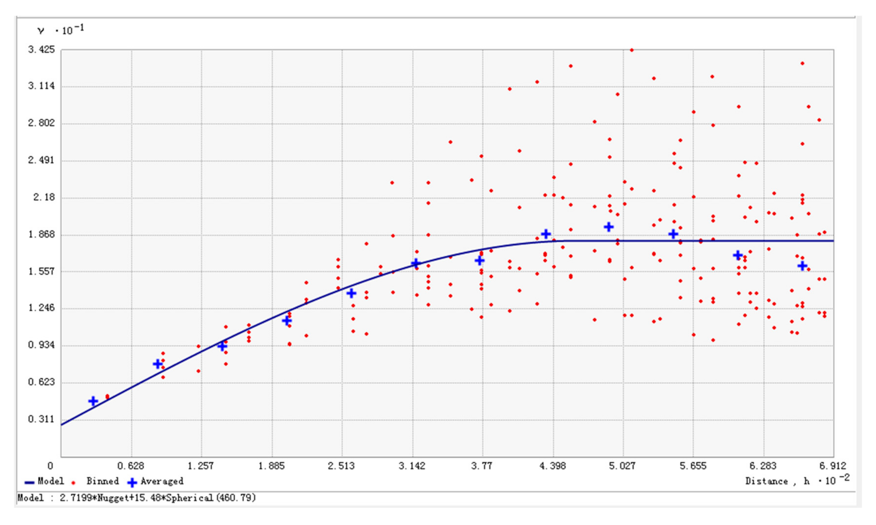
According to the removal-recovery method, low-density data need to be converted into high-density data first, in order to avoid the impact of density differences. In this study, a 150 by 150 m grid was generated by the ordinary kriging interpolation method for all data, which has been widely used in the interpolation of underwater topography of reservoirs and lakes. The method was based on the spherical semi-variogram model, and the model parameter, nugget, and partial sill were optimized using cross-validation with a focus on the estimation of the range parameter by using the Geostatistical Analyst tools in ArcGIS. Then, the generated grid was resampled and encrypted into 50 by 50 m grid data, which were used as the reference grid. Subsequently, a 50 by 50 m grid by high-density data itself was interpolated to generate the high-resolution grid data. Finally, the remove-restore method was employed to merge the reference grid and the high-resolution grid as follows: (1) comparing the elevation of the reference grid with that of the high-resolution grid, calculating the difference between them, and generating the difference file; (2) correcting the reference grid based on the difference file; and (3) combining the revised reference grid and the high-density data to re-interpolated for obtaining the final terrain results. Figure 4 shows the curve of semi-variogram model.
It can be seen that pairs of locations that are closer have more similar values. As pairs of locations become farther apart, they become more dissimilar and have a higher squared difference. The nugget is 2.7199, the major range is 460.79, and the partial sill is 15.4802. The ratio of nugget to sill is 14.94%, means that the system has a strong spatial correlation.
3.5. Error Analysis of Interpolation Methods
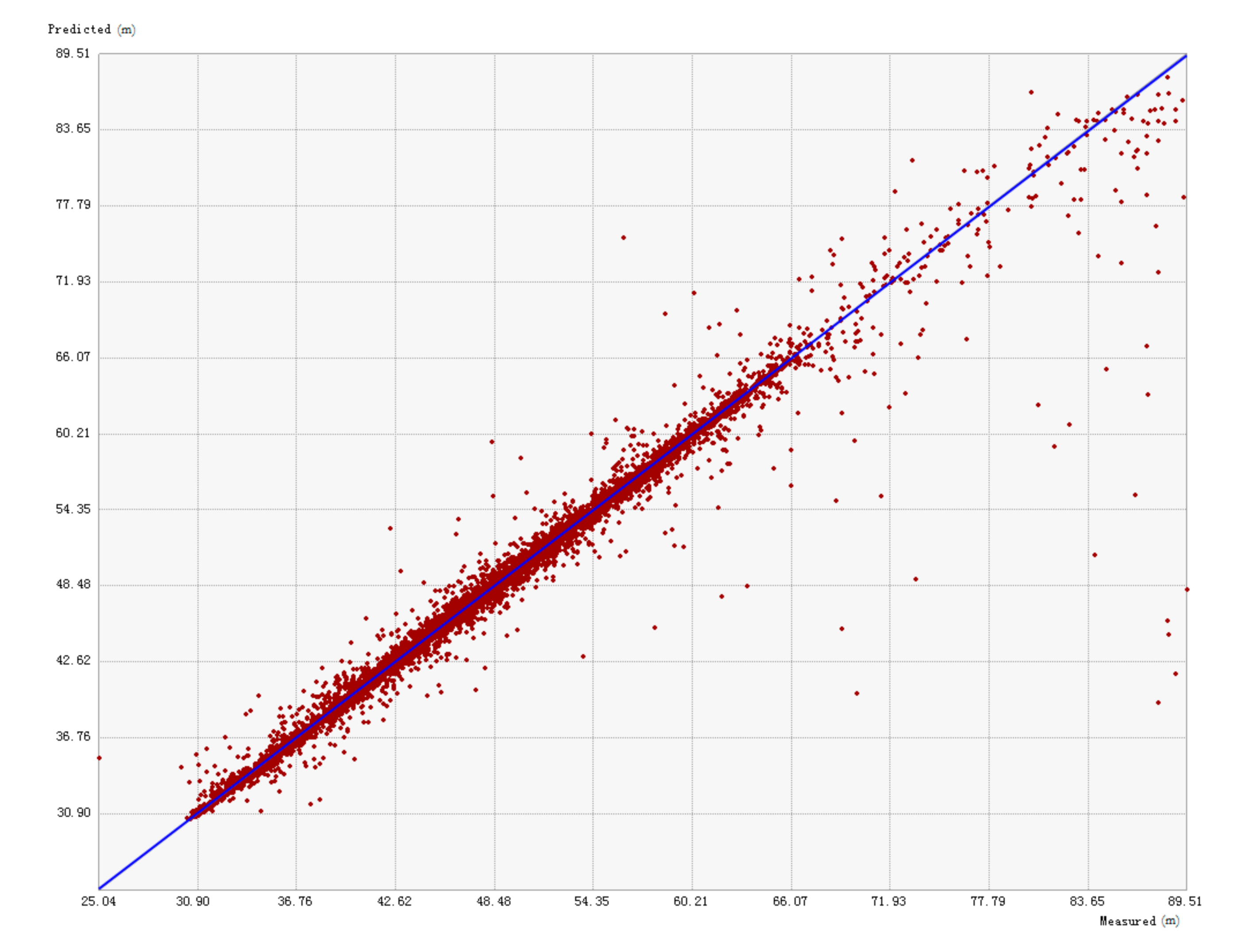
The interpolation calculation involves errors, which will affect the accuracy of the results. This paper uses a cross-validation method to evaluate the uncertainty of the simulation result of the reservoir. Figure 5 shows the results of the cross-validation between predicted and measured values.
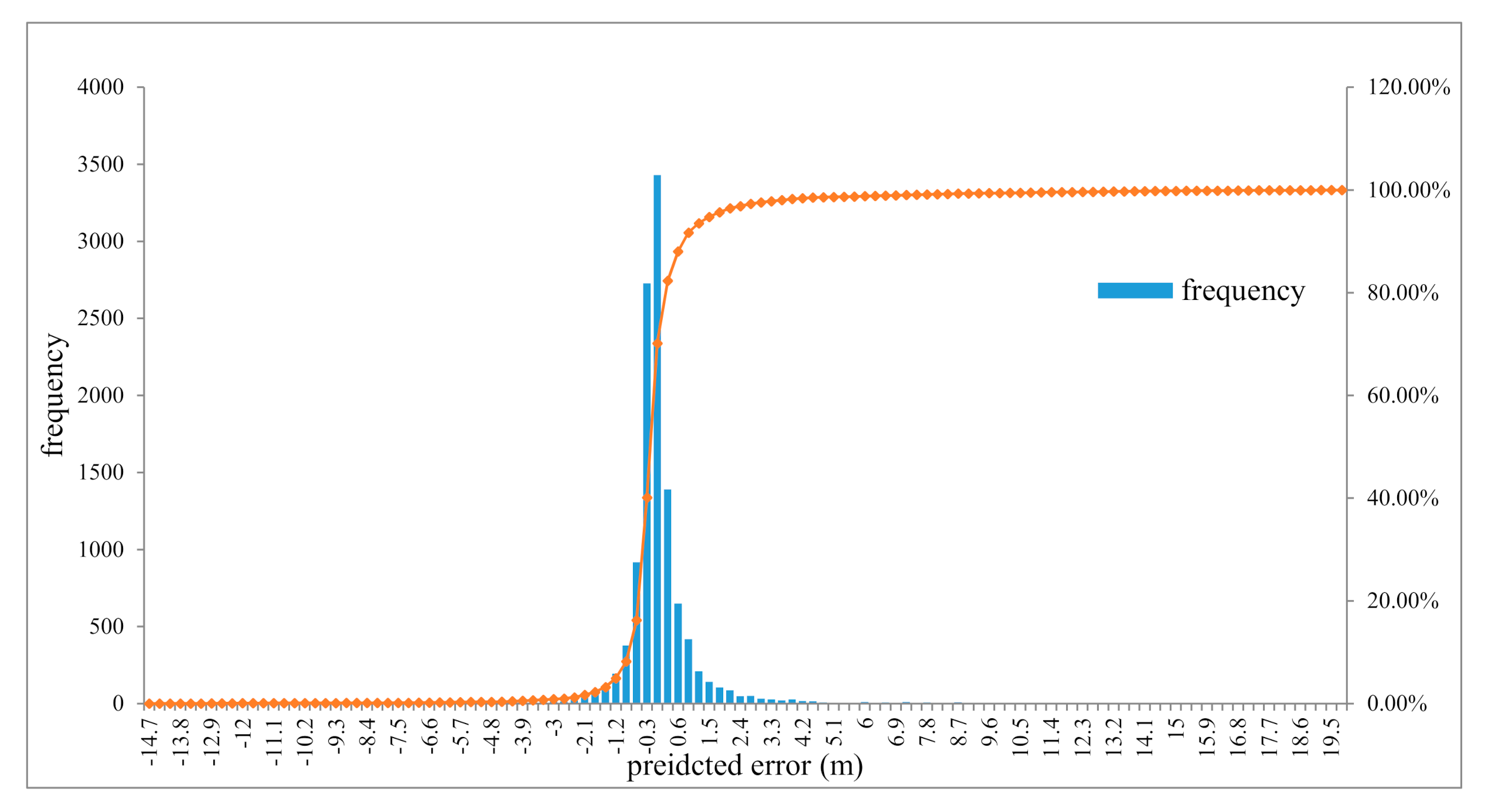
Figure 6 and Figure 7 are the histogram of prediction error and the spatial distribution of prediction error, respectively. As can be seen from Figure 6, the prediction errors are concentrated between −0.6 and 0.3 m, with an average prediction error of −0.029 m. From Figure 7, it can be seen that the errors greater than 0.3 m are mostly distributed in the reservoir edge and the inflow section of small tributaries, which are mainly due to the low data density and the rapid change of the terrain conditions over a short distance. By comparing with the original data distribution map, it can be found that the regional error of the high density of the original data in the reservoir is mostly within 0.3 m; the prediction error along the track point data is even less than 0.1 m. Thus, the prediction error of the fusion method is related to the degree of terrain changes and data density.
4. Results and Analysis
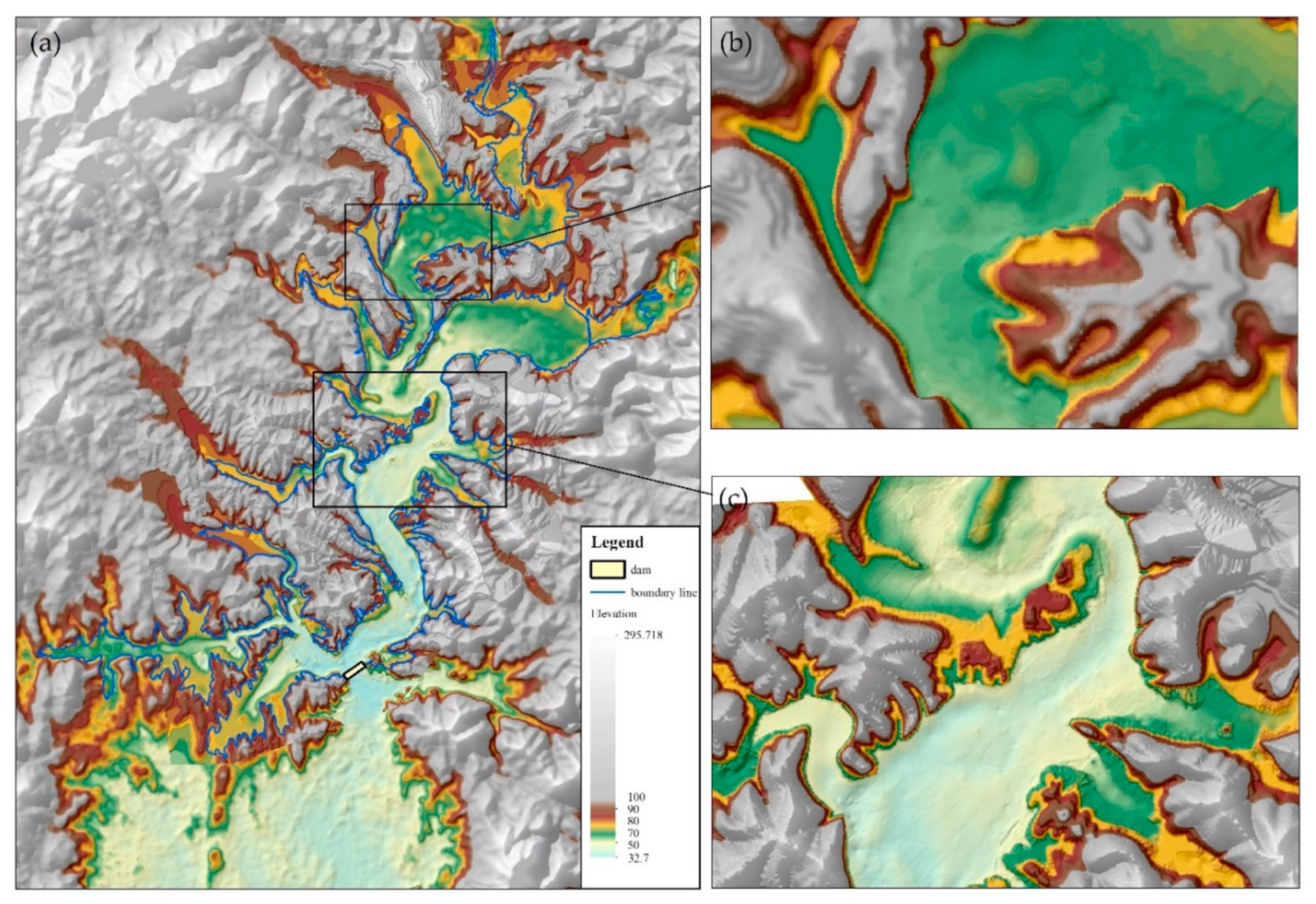
Figure 8 shows the bottom topography of the reservoir in this study, which is generated by the multi-source data fusion method. It looks natural and smooth in the areas where the original data is relatively sparse and obsolete, especially in the areas adjacent to the high-precision data (Figure 8b). Meanwhile, in the area with a high density of original data, the interpolation accuracy is retained, and the position and direction of the original river before the construction of the reservoir can be identified accurately and clearly (Figure 8c). This proves that the multi-source data fusion method proposed in this paper can preserve the accuracy and characteristics of high density and strong timeliness data in the process of terrain interpolation and also avoid the distortion of results caused by the interference of low density and weak timeliness data due to the nearby high accuracy data.
4.1. Comparison of Multi Method Results
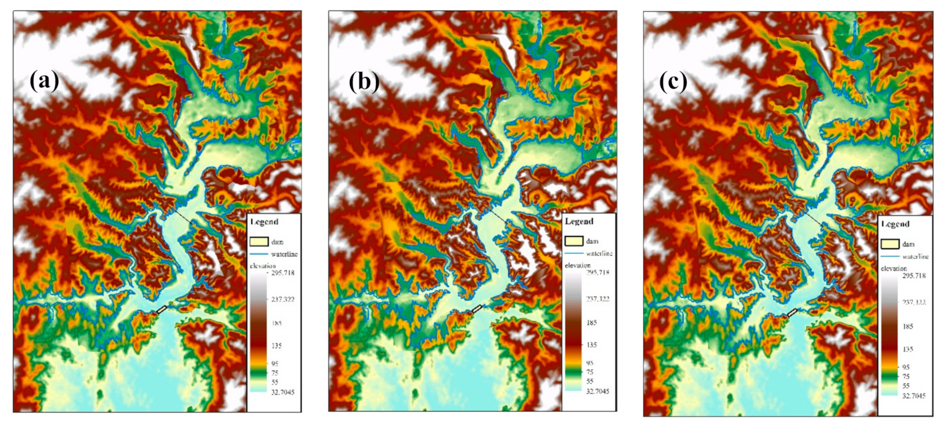
As mentioned before, the terrain simulation method based on multi-source data fusion has been widely used in marine areas. On the basis of existing methods, in this paper, we proposed an improved multi-source data fusion method, which considered the distinctive characteristics of reservoir topography. To test the difference between this improved method and other terrain simulation methods, the widely used ordinary kriging interpolation method and the existing multi-source data fusion method applied in the marine field, were used for terrain interpolation in the reservoir area [30,31]. The ordinary kriging method was based on the spherical semi-variogram model, and the parameter, nugget, and partial sill were optimized by using the Geostatistical Analyst tools in ArcGIS. The results of the three methods are shown in Figure 9.
To verify the effectiveness of the improved multi-source data fusion method for eliminating errors due to data differences, the simulation results were compared and analyzed in detail, as shown in Figure 10.
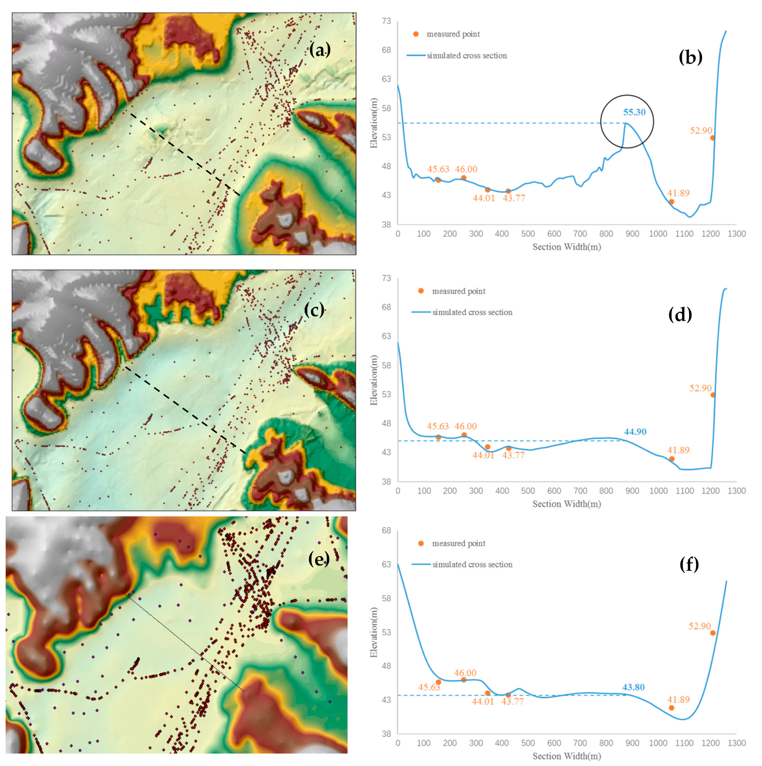
Because of the different densities and precision of the original data, the low-density data area is easily distorted by the high-density data area nearby when using the conventional interpolation method, generating unnatural bulges or depressions. According to the interpolation results of the standard kriging interpolation method (Figure 10a) and the improved multi-source data fusion method (Figure 10b) in the section of reservoir center, we can see that the surface obtained by the standard Kriging interpolation method has an irregular block structure, while the surface obtained by the improved multi-source data fusion method is more natural and smooth. Figure 10b,d are profiles generated by two methods in the section of reservoir center. It can be seen that the extreme elevation of 55.3 m is generated by the standard kriging method at the location shown in Figure 10b, due to the influence of the high-density data near the left bank and downstream. Compared with other measured elevation values in the same section, it can be inferred that the predictive value of 55.3 m is abnormal. The interpolation result using the improved method at the same position is only 44.9 m, which is closer to the measured value in the same section. It suggests that the improved multi-source data fusion method has less error than the standard kriging method when generating terrain.
Changes of seabed terrain in the ocean area are evaluated on a scale of tens of thousands of years, therefore, terrain data acquired with an interval of several decades does not introduce a significant difference in accuracy. In contrast, regarding operation of a reservoir, the topography of a reservoir can experience a marked change in several decades. Thus, when directly applying the multi-source fusion method for oceans to reservoirs, the uncorrected old data lead to deviation of the results. Figure 10e is the interpolation result and Figure 10f is the profile of the result in the section using the non-time difference correction fusion method. It can be seen that there is deviation between the interpolation results of the non-time difference correction fusion method and the measured results is substantially high. The farther the interpolated point is from the track point, the greater the error is. This suggests that the improved multi-source data fusion method can simulate the terrain of the reservoir area more accurately.
4.2. Verification of Precision
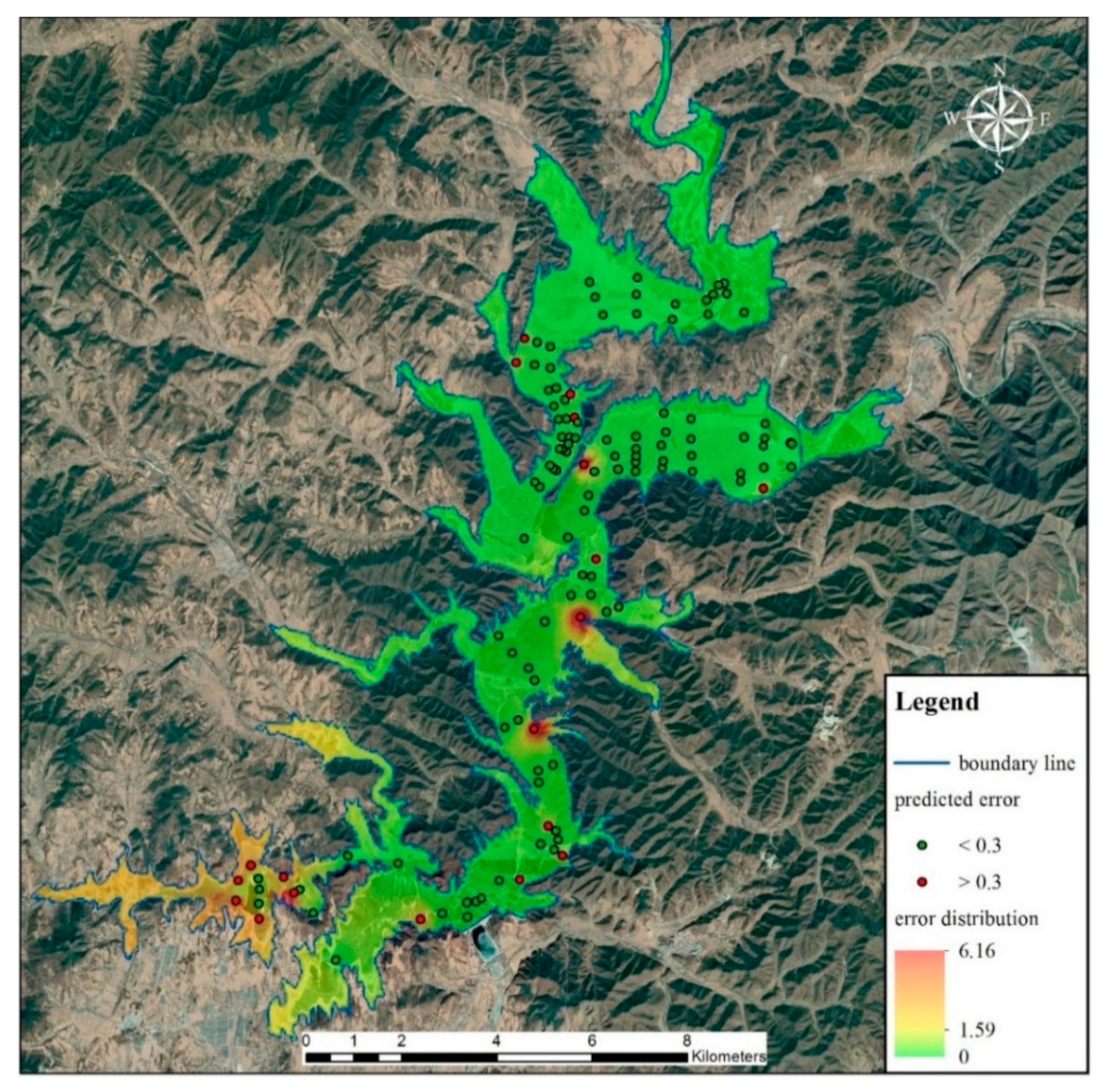
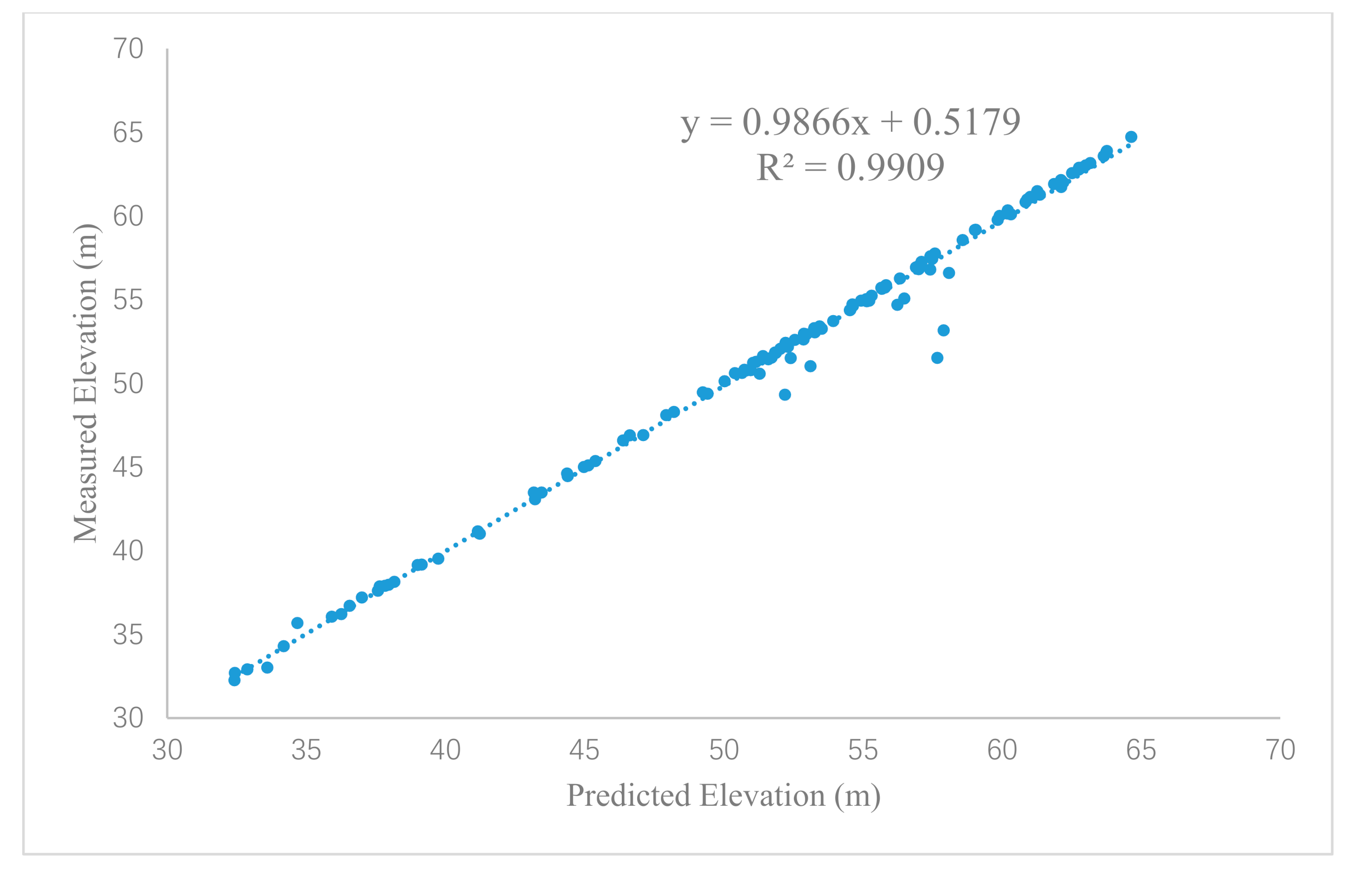
In order to verify the reliability of the final updating terrain, we use the topographic data measured by the project team in the reservoir site to verify the results (Figure 11). These were the latest field survey data of the project team in 2017, which was not used in the calculation of terrain simulation. First, we overlay the measured data points with the DEM of the base terrain of the simulation results by georeferencing. Then, we extract the simulated elevation values at the corresponding locations to the points. Finally, we analyze the correlation between the simulated elevation value and the measured one of each data point. The results are shown in Figure 12. Meanwhile, the mean error and root mean square error (RMSE) between the simulated and measured values of the selected verification points are calculated (Table 1), which is used to analyze the accuracy of the terrain simulation.
Correlation analysis shows that there is a significant linear correlation between simulated elevation and measured elevation (R2 = 0.9909). The average simulation error of each verification point is 0.291 m, the average error percent is 0.56%, and the root mean square error is 0.752 m. It suggests that the simulation results can, overall, better reflect the actual topographic conditions, but there are a few extreme points with large errors. By combining the distribution of verification points and the prediction error (Figure 11), the points with greater simulation deviations can be seen in two types of areas.
The first type distributes in the water-land boundary area of the reservoir margin. Because the reservoir margin is mostly steep mountain slopes and the elevation change rate in this area is great, the interpolation error increases accordingly. In addition, because the old topographic map was produced a long time ago, there were some errors in georeferencing with new data. Generally, the closer to the boundary, the lower the accuracy of georeferencing. Those factors lead to the larger simulation errors of such points.
The second type is concentrated in the southwest of the reservoir. In recent years, sand mining in this area has seriously damaged the original terrain, and the original elevation data in this area is deficient, especially the lack of high precision and time-sensitive elevation data, which results in large errors between the simulated terrain and the measured one.
4.3. Rationality Assessment
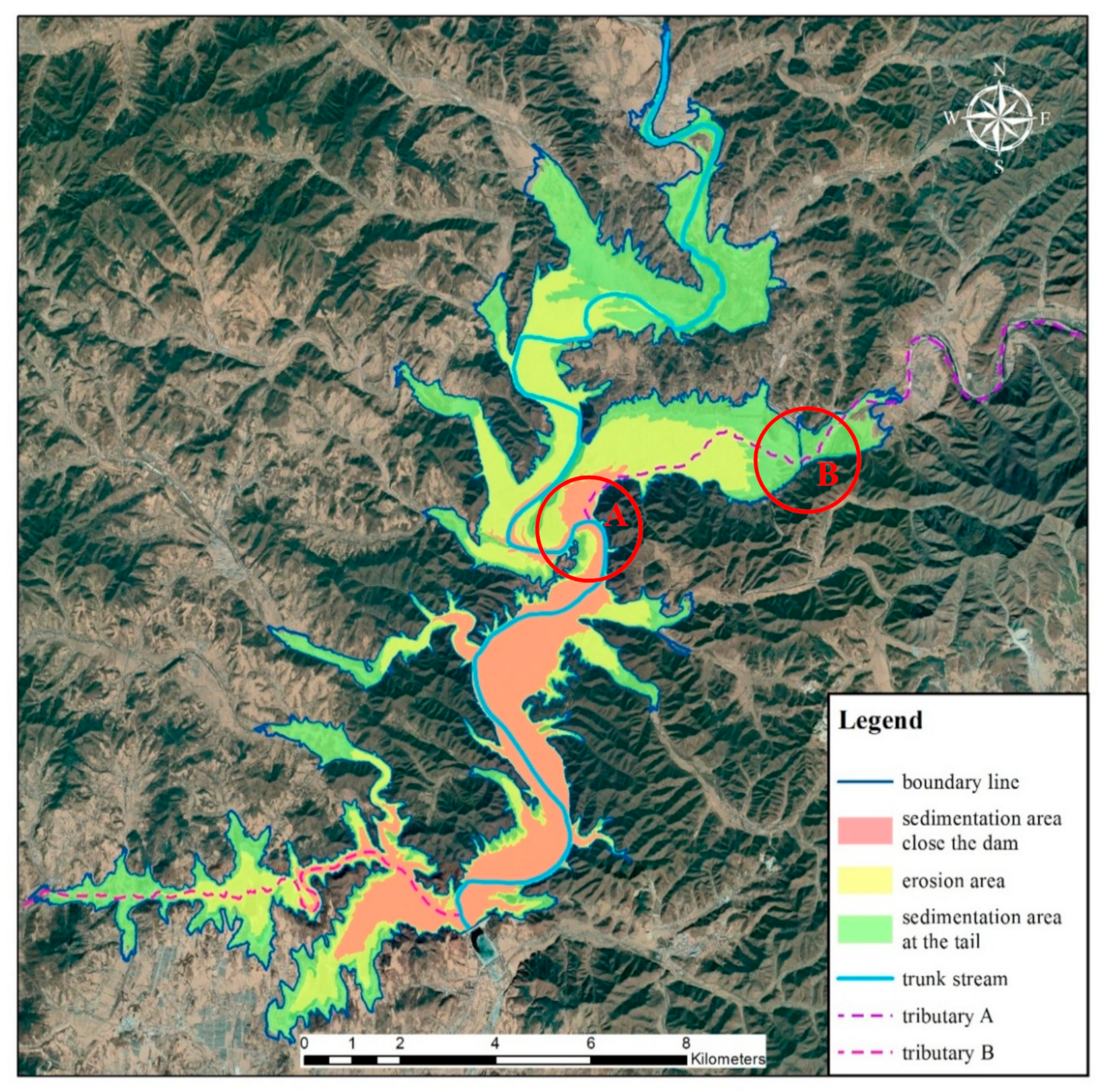
In order to verify the accuracy of the topographic simulation results of the reservoir in this study, the satellite images (2017) of the upstream backwater area of the reservoir, during the period of barrenness, were used to represent the actual topography, and the hydrological analysis method was used to evaluate the difference between the actual situations after topographic updating of the reservoir. Firstly, the hydrological analysis and calculation of the reservoir topography after the updating were carried out using ArcGIS software, and the river networks were extracted. Then, the extracted river networks were overlaid with satellite images of the upstream backwater area of the reservoir. Finally, by comparing the extracted river networks and the actual river channels on the satellite images, the degree of deviation of updated terrain to the actual situation was evaluated, as shown in Figure 13.
It can be found that the river networks extracted from the updated terrain have a good coincidence with the real river channel on the satellite images. In the whole warehousing section, the extracted river course coincides with the actual one, only some deviations are found in locations A and B (Figure 13). We conclude that the simulated new terrain reflects the real reservoir terrain reasonably well. This also suggests that the proposed fusion method can reasonably accurately update the underwater topography of the reservoir.
4.4. Estimation of Erosion and Sedimentation of the Reservoir
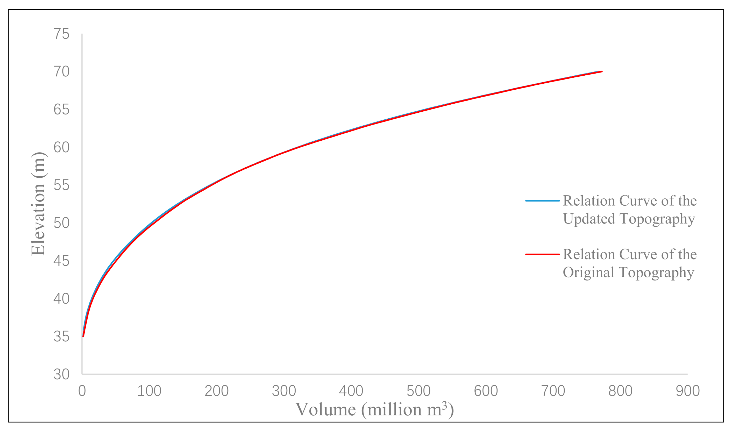
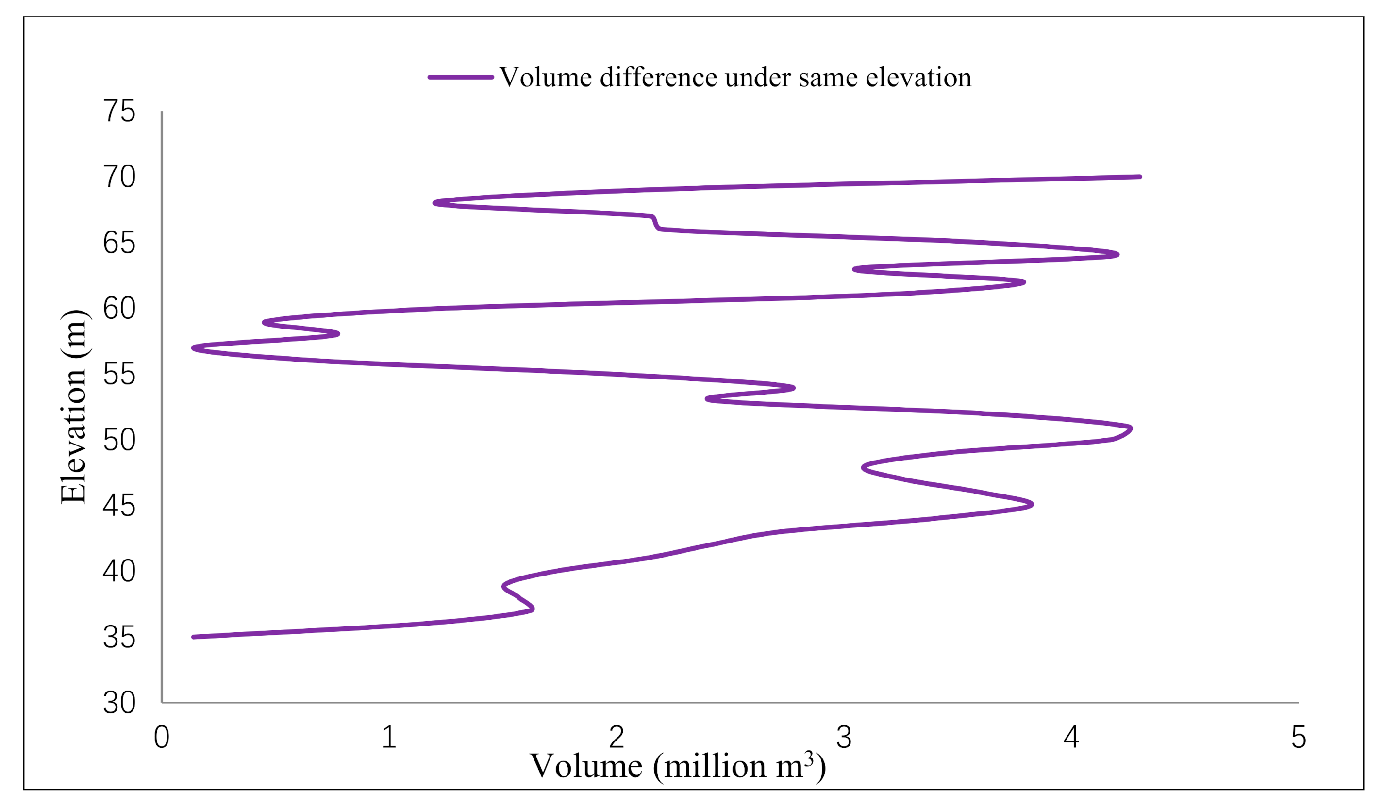
Siltation reduces the effective storage capacity of the reservoir, and also has an adverse impact on water quality. The surface volume tool in ArcGIS can calculate the volume between the topographic map and a reference plane, which could be used to develop the elevation and volume relationship curve. With this tool, we developed the elevation and volume relation curves of both the original topographic map and the updated topographic map (Figure 14). By subtracting the curve of the updated terrain from the curve of the original topographic map, we obtained the difference curve (Figure 15).
In Figure 15, the difference curve is always above the value of 0, which indicates that the volume of terrain calculated after updating is smaller than that before updating. This is consistent with the fact that the reservoir capacity decreases with the increase of operation time, which suggests that the calculation result is reasonable.
Furthermore, the difference curve could be used to roughly infer the total volume of siltation. By examining the historical water level data of the reservoir, we found that the highest water level was 69.67 m. The volume difference under 69.67 m could be regarded as the total siltation in the reservoir, which was 4.3 million m3 according to the difference curve. It can be seen that the volume difference fluctuates with the change of water level (Figure 15), which is caused by silting or erosion in the different areas of the reservoir. We divided the water level into 14 zones. The volume of sedimentation/erosion in each zone is shown in Figure 16. It is noted that the negative values refer to the volume of erosion and the positive values refer to the volume of siltation. Correspondingly, the spatial distribution of erosion/sedimentation in the reservoir is shown in Figure 17.
As shown in Figure 17, the reservoir could be roughly divided into three areas: the sedimentation area at the tail of the reservoir, submerged at water level between 60 and 70 m; the erosion area, submerged at water level between 50 and 60 m; and the sedimentation area in the front of the dam, submerged at a water level of 50 m. The formation of the siltation area at the tail of the reservoir is mainly due to the slowdown of flow velocity and the decrease of sediment carrying capacity of flow caused by the rapid expansion of the flow section after the river enters the reservoir. The river channel at the elevations between 50 and 60 m has a narrower cross-section and steeper bed gradients than upstream and downstream, causing channel erosion. The eroded sediments that are carried by river flow deposit in the frontal area of the dam, forming a siltation area below 50 m elevation. In addition, there are still two scouring zones, the elevation of one zone is between 45 and 47.5 m and the elevation of the other zone is between 65 and 67.5 m. The former is located at the junction of the trunk steam of the reservoir and its tributary A (at A in Figure 17). The latter mainly distributes in the upstream of each tributary and the vicinity of river-crossing bridge of tributary A (at B in Figure 17). The upstream and downstream of the bridge cave are heavily scoured by flood water. Thus, the spatial distribution of siltation and erosion in reservoirs is very complicated, and affected by hydrological conditions, the topography of reservoir bottom, and the shape of reservoir area, among others.
5. Conclusions
Due to erosion and siltation, the topography of a reservoir bottom experiences rapid changes after decades of operation. Thus, terrain data of a reservoir bottom should be updated in time to ensure safe operation of a reservoir. In this paper, we developed a multi-source terrain data fusion method. This method was applied to update the topographic map of a reservoir in Northeast China by integrating the existing data of sonar detection, historical topographic map, and so on. A comparison with direct measurement data showed that updated terrains using this method could reasonably reflect the actual topography of a reservoir area. Furthermore, changing volumes of erosion and deposition were calculated and their spatial distribution in a reservoir area was mapped, which could provide practical guidance in reservoir management.
Author Contributions
Conceptualization, S.X. and Y.L.; methodology, Y.L. and T.W.; software, Y.L.; validation, S.X. and Y.L.; investigation, Y.L. and T.W.; resources, S.X.; writing—original draft preparation, Y.L.; writing—review and editing, S.X. and T.Z.; supervision, S.X. All authors have read and agreed to the published version of the manuscript.
Funding
This research was supported by the National Natural Science Foundation of China, grant number 51879031.
Conflicts of Interest
The authors declare no conflict of interest.
References
- Perera, B.J.C.; Codner, G.P. Reservoir targets for urban water supply systems. J. Water Resour. Plan. Manag. 1996, 122, 270–279. [Google Scholar] [CrossRef]
- Palanques, A.; Grimalt, J.; Belzunces, M.; Estrada, F.; Puig, P.; Guillén, J. Massive accumulation of highly polluted sedimentary deposits by river damming. Sci. Total Environ. 2014, 497, 369–381. [Google Scholar] [CrossRef] [PubMed]
- Atici, T.; Ahiska, S.; Altindag, A.; Aydin, D. Ecological effects of some heavy metals (Cd, Pb, Hg, Cr) pollution of phytoplanktonic algae and zooplanktonic organisms in Sarýyar Dam Reservoir in Turkey. Afr. J. Biotechnol. 2008, 7, 1972–1977. [Google Scholar]
- Wei, G.L.; Yang, Z.F.; Cui, B.S.; Li, B.; Chen, H.; Bai, J.H.; Dong, S.K. Impact of Dam Construction on Water Quality and Water Self-Purification Capacity of the Lancang River, China. Water Resour. Manag. 2009, 23, 1763–1780. [Google Scholar] [CrossRef]
- Beletsky, D.; chwab, D.J. Modeling circulation and thermal structure in Lake Michigan: Annual cycle and interannual variability. J. Geophys. Res. Ocean. 2001, 106, 19745–19771. [Google Scholar] [CrossRef] [Green Version]
- Charles, J.A. The engineering behavior of fill materials and its influence on the performance of embankment dams. Dams Reservoirs. 2009, 19, 21–33. [Google Scholar] [CrossRef]
- Gaytán, R.; Anda, J.; Nelson, J. Computation of changes in the run-off regimen of the Lake Santa Ana watershed (Zacatecas, México). Lakes Reserv. Res. Manag. 2008, 13, 155–167. [Google Scholar] [CrossRef]
- Liu, Z.C.; Zhou, X.H.; Chen, Y.L.; Hu, G.H. The Development in the Latest Technique of Shallow Water Multi-beam Sounding System. Hydrogr. Surv. Charting 2005, 25, 67–70. [Google Scholar]
- Momber, G.; Geen, M. The application of the Submetrix ISIS-100 Swath Bathymetry system to the management of underwater sites. Int. J. Naut. Archaeol. 2000, 29, 154–162. [Google Scholar] [CrossRef]
- Gourlay, T.P.; Cray, W.G. Ship under-keel clearance monitoring using RTK GPS. Coasts Ports 2009 Dyn. Environ. 2009, 376. [Google Scholar]
- Ceylan, A.; Karabork, H.; Ekozoglu. I. An analysis of bathymetric changes in Altinapa reservoir. Carpathian J. Earth Environ. Sci. 2011, 6, 15–24. [Google Scholar]
- Noernberg, M.A.; Krug, L.A. Remote sensing and GIS integration for modelling the Paranaguá estuarine complex- Brazil. J. Coast. Res. 2006, 39, 1627–1631. [Google Scholar]
- Lafon, V.; Froidefond, J.M.; Lahet, F.; Castaing, P. Spot shallow water bathymetry of a moderately turbid tidal inlet based on field measurements. Remote Sens. Environ. 2002, 81, 136–148. [Google Scholar] [CrossRef]
- Brando, V.E.; Anstee, J.M.; Wettle, M.; Dekker, A.G.; Phinn, S.R.; Roelfsema, C. A physics based retrieval and quality assessment of bathymetry from suboptimal hyperspectral data. Remote Sens. Environ. 2009, 113, 755–770. [Google Scholar] [CrossRef]
- Alcantara, E.; Novo, E.; Stech, J.; Assireu, A.; Nascimento, R.; Lorenzzetti, J.; Souza, A. Integrating historical topographic maps and SRTM data to derive the bathymetry of a topical reservoir. J. Hydrol. 2010, 389, 311–316. [Google Scholar] [CrossRef] [Green Version]
- Gueriot, D. Bathymetric and side-scan data fusion for sea-bottom 3D mosaicking. In Proceedings of the OCEANS 2000 MTS/IEEE Conference and Exhibition, Providence, RI, USA, 11–14 September 2000; IEEE: Piscataway, NJ, USA, 2000; Volume 3, pp. 1663–1668. [Google Scholar]
- Zhang, C. Applying data fusion techniques for benthic habitat mapping and monitoring in a coral reef ecosystem. Isprs J. Photogramm. Remote Sens. 2015, 104, 213–223. [Google Scholar] [CrossRef]
- Jha, S.K.; Mariethoz, G.; Kelly, B.F.J. Bathymetry fusion using multiple-point geostatistics: Novelty and challenges in representing non-stationary bedforms. Environ. Modell. Software 2013, 50, 66–76. [Google Scholar] [CrossRef]
- Shen, J.; Su, T.Y.; Wang, G.Y.; Liu, H.X.; Li, J.G. Submarine topography visualization based on Kriging algorithm, Mar. Sci. 2012, 36, 24–28. [Google Scholar]
- Yu, H.J.; Wu, C.Y.; Zhou, J.Y.; Gao, L.; Li, Y.C. Study of Multi-Source Data DEM Production, J. Geomat. 2016, 41, 86–88. [Google Scholar]
- Arndt, J.E.; Schenke, H.W.; Jakobsson, M.; Nitsche, F.O.; Buys, G.; Goleby, B.; Rebesco, M.; Bohoyo, F.; Hong, J.; Black, J.; et al. The International Bathymetric Chart of the Southern Ocean (IBCSO) Version 1.0—A new bathymetric compilation covering circum-antarctic waters. Geophys. Res. Lett. 2013, 40, 3111–3117. [Google Scholar] [CrossRef] [Green Version]
- Fan, M.; Sun, Y.; Xing, Z.; Wang, Y.; Jin, J. Bathymetry fusion techniques for high-resolution digital bathymetric modeling, Acta Oceanol. Sin. 2017, 39, 130–137. [Google Scholar]
- Kondolf, G.M.; Gao, Y.; Annandale, G.W.; Morris, G.L.; Jiang, E.; Zhang, J.; Hotchkiss, R. Sustainable sediment management in reservoirs and regulated rivers: Experiences from five continents. Earth’s Future 2014, 2, 256–280. [Google Scholar] [CrossRef]
- Casado, A.; Hortobágyi, B.; Roussel, E. Historic reconstruction of reservoir topography using contour line interpolation and structure from motion photogrammetry. Int. J. Geogr. Inf. Sci. 2018, 32, 2427–2446. [Google Scholar] [CrossRef]
- Jia-shang, S.H.A.N.G. Application and the Comparison of the Difference Method and the Ratio Method in the Correction of the Error. Metrol. Meas. Technol. 2009, 4, 25. [Google Scholar]
- Forsberg, R.; Tscherning, C.C. The use of height data in gravity field approximation by collocation. J. Geophys. Res. Solid Earth 1981, 86, 7843–7854. [Google Scholar] [CrossRef]
- Hell, B.; Jakobsson, M. Gridding heterogeneous bathymetric data sets with stacked continuous curvature splines in tension, Mar. Geophys. Res. 2011, 32, 493–501. [Google Scholar]
- Zhu, L.; Liu, J.W.; Xu, S.G.; Xie, Z.G. Deposition behavior, risk assessment and source identification of heavy metals in reservoir sediments of Northeast China. Ecotoxicol. Environ. Saf. 2017, 142, 454–463. [Google Scholar] [CrossRef]
- Hobo, N.; Makaske, B.; Middelkoop, H.; Wallinga, J. Reconstruction of sedimentation rates in embanked floodplains, a comparison of four methods. NCR Days 2008, 2008, 80. [Google Scholar]
- Aykut, N.O.; Akpinar, B.; Aydin, Ö. Hydrographic Data Modeling Methods for Determining Precise Seafloor Topography. Comput. Geosci. 2013, 13, 661–669. [Google Scholar] [CrossRef]
- Hamidi, M.J.E.; Larabi, A.; Faouzi, M.; Souissi, M. Spatial distribution of regionalized variables on reservoirs and groundwater resources based on geostatistical analysis using GIS: Case of Rmel-Oulad Ogbane aquifers (Larache, NW Morocco). Arab. J. Geosci. 2018, 11, 104. [Google Scholar] [CrossRef]
Figure 1.
Location of the studied reservoir.

Figure 2.
Study area and the distribution of multi-source data.

Figure 3.
The flowchart of multi-source terrain data fusion method.

Figure 4.
The semi-variogram model curve.

Figure 5.
Cross-validation analysis results of kriging interpolation.

Figure 6.
Histogram of prediction error.

Figure 7.
Spatial distribution of prediction error.

Figure 8.
The results of the simulated terrain. (a) The overall display of the result; (b) Interpolation display of the low data density area; (c) Interpolation display of the high data density area.
Figure 8.
The results of the simulated terrain. (a) The overall display of the result; (b) Interpolation display of the low data density area; (c) Interpolation display of the high data density area.

Figure 9.
Results of different terrain simulation methods. (a) Standard kriging interpolation method; (b) The existing multi-source data fusion method; (c) The improved multi-source data fusion method.
Figure 9.
Results of different terrain simulation methods. (a) Standard kriging interpolation method; (b) The existing multi-source data fusion method; (c) The improved multi-source data fusion method.

Figure 10.
Comparison of the results using different methods. (a) The standard kriging method; (b) A section of the standard kriging method; (c) The improved multi-source data fusion method; (d) A section of the improved multi-source data fusion method; (e) The existing multi-source data fusion method; (f) A section of the existing multi-source data fusion method.

Figure 11.
Distribution of the verification points and the prediction error.

Figure 12.
Distribution of the verification points and the prediction error.

Figure 13.
Contrast between the satellite image and the river network of the updated terrain (locations A and B: the examples for deviations).
Figure 13.
Contrast between the satellite image and the river network of the updated terrain (locations A and B: the examples for deviations).

Figure 14.
The elevation and volume relation curves of the original and the updated topography.

Figure 15.
Relation curve of volume difference under same elevation.

Figure 16.
Erosion and sedimentation characteristics in different zones of the reservoir.

Figure 17.
Spatial distribution of erosion and sedimentation areas in the reservoir.


Table 1.
Contrast result of measured value and predicted value of the verification points.
| No. | Measured (m) | Predicted (m) | Error (m) | Error Percent | |
|---|---|---|---|---|---|
| 1 | 41.154 | 41.163 | 0.009 | 0.02% | |
| 2 | 38.138 | 38.159 | 0.021 | 0.06% | |
| 3 | 39.140 | 39.002 | 0.138 | 0.35% | |
| 4 | 32.902 | 32.874 | 0.028 | 0.08% | |
| 5 | 36.051 | 35.913 | 0.138 | 0.38% | |
| 6 | 32.253 | 32.412 | 0.159 | 0.49% | |
| … | … | … | … | … | |
| 123 | 44.447 | 44.374 | 0.056 | 0.13% | |
| 124 | 41.004 | 41.301 | 0.229 | 0.56% | |
| Max error | 6.160 | R2 | 0.9909 | Average error | 0.291 |
| Min error | 0.003 | RMSE | 0.752 | Average error percent | 0.56% |
Publisher’s Note: MDPI stays neutral with regard to jurisdictional claims in published maps and institutional affiliations. |
© 2020 by the authors. Licensee MDPI, Basel, Switzerland. This article is an open access article distributed under the terms and conditions of the Creative Commons Attribution (CC BY) license (http://creativecommons.org/licenses/by/4.0/).
Share and Cite
MDPI and ACS Style
Liu, Y.; Xu, S.; Zhu, T.; Wang, T. Application of Multi-Source Data Fusion Method in Updating Topography and Estimating Sedimentation of the Reservoir. Water 2020, 12, 3057. https://doi.org/10.3390/w12113057
AMA Style
Liu Y, Xu S, Zhu T, Wang T. Application of Multi-Source Data Fusion Method in Updating Topography and Estimating Sedimentation of the Reservoir. Water. 2020; 12(11):3057. https://doi.org/10.3390/w12113057
Chicago/Turabian StyleLiu, Yu, Shiguo Xu, Tongxin Zhu, and Tianxiang Wang. 2020. "Application of Multi-Source Data Fusion Method in Updating Topography and Estimating Sedimentation of the Reservoir" Water 12, no. 11: 3057. https://doi.org/10.3390/w12113057
Note that from the first issue of 2016, this journal uses article numbers instead of page numbers. See further details here.