Comparison of Ensembles Projections of Rainfall from Four Bias Correction Methods over Nigeria


1
Department of Civil Engineering, Seoul National University of Science and Technology, Seoul 01811, Korea
2
Department of Environmental Sciences, Faculty of Science, Federal University Dutse, Dutse P.M.B 7156, Nigeria
*
Author to whom correspondence should be addressed.
Water 2020, 12(11), 3044; https://doi.org/10.3390/w12113044
Submission received: 17 September 2020
/
Revised: 21 October 2020
/
Accepted: 28 October 2020
/
Published: 30 October 2020
(This article belongs to the Section Hydrology)
Abstract
:This study compares multi model ensemble (MME) projections of rainfall using general quantile mapping, gamma quantile mapping, Power Transformation and Linear Scaling bias correction (BC) methods for representative concentration pathways (RCPs) 4.5 and 8.5 of the Coupled Model Intercomparison Project phase 5 (CMIP5) global climate models (GCMs). Using the Global Precipitation Climatology Centre historical period (1961–2005) rainfall data as the reference, projection was conducted over 323 grid points of Nigeria for the periods 2010–2039, 2040–2069 and 2070–2099. The performances of the different BC methods in removing biases from the GCMs were assessed using different statistical indices. The computation of the MME of the projected rainfall was conducted by aggregation of 20 GCMs using random forest regression method. The percentage differences in the future rainfall relative to the historical period were estimated for all BC methods. Spatial projection of the percentage changes in rainfall for Linear scaling, which was the best performing BC method, showed increases in rainfall of 5.5–6.9% under RCPs 4.5 and 8.5, respectively, while the decrease range was −3.2–−4.2% respectively during the wet season. The range of annual increases in precipitation was 5.7–7.3% for RCP 4.5 and 8.5, respectively, while the decrease range was −1.0–−4.3%. This study also revealed monthly rainfall within the country will decrease during the wet season between June and September, which is a significant period where most crops need the water for growth. Findings from this study can be of importance to policy makers in the management of changes in hydrological processes due to climate change and management of related disasters such as floods and droughts.
1. Introduction
Rainfall is an important component of the climatic and hydrological system as it is the primary source that replenishes different water sources around the globe. There is natural variability in the period and amount of rainfall received across the globe. However, the many decades of greenhouse gases emissions (GHG) have aggravated the dynamism of the climate of the earth, which has in recent times resulted in more erratic seasonal and annual rainfall in many parts of the globe [1,2,3,4]. This has subsequently affected the intensity, frequency and risk of disasters which have been projected to increase in the future [5,6,7,8,9,10]. For example, the climatology of global drought conditions under different global warming levels was investigated [11]. The study showed that, for drying areas, the duration of droughts is going to rise at an increasingly rapid rate with warming, averaged globally from 2.0 month/°C to 4.2 month/°C. These warming conditions are expected to affect two thirds of the global population. Therefore, there is a need for further understanding of the expected changes regionally and particularly in understudied regions in parts of Africa where agricultural yields can be affected by decrease in rainfall.
Recently, with advancements in artificial intelligence and machine learning, prediction of the expected changes to the climate of the earth has been possible [12,13]. In general, climate projections have been conducted using global climate models (GCMs), historical and future climate simulations at global scales for understanding the expected changes in the climate. While they can be applied at global scale in their original resolution, their direct application at regional or local scale can affect the outputs of climate studies. It is therefore essential to downscale them using either statistical or dynamical downscaling methods. The statistical downscaling method compared to the dynamical are widely used due to their strength of incorporation of observations directly into methods, their computational and cost effectiveness and their provision of point-scale climatic projections from GCM-scale output [14,15,16].
GCMs are produced by different organizations, so they have different configurations and module characteristics, which give them variation in their temporal and spatial performances across the globe [8,17,18] which makes a choice of GCMs to apply in climate studies arduous. On the other hand, it has been reported that all climate models are treated as having equal performances due to the similarity in their behaviors [19]. Ensemble prediction systems (EPS) are being increasingly applied in atmospheric and hydrologic models [20]. Ensemble rainfall projections can be of significant interest in decision making, due to provision of an explicit and dynamic assessment of the uncertainties associate with the projections [21]. To further address the issue of uncertainties in climate and hydrological projections, an approach that involves the generation of a multi model ensemble (MME) from a number of models has been applied in many studies [17,22]. Aggregation of GCMs into MME can involve selection of some number of models based on weighting [23,24] or the non-weighing approach in which models are aggregated directly into an MME based on choices [22].
Aside from the uncertainties associated with the different GCMs, downscaling methods used for the removal of biases in GCMs have been found to be sources of uncertainties in climate studies [25,26]. For example, Sharma et al. [27] evaluated the uncertainty that arises during climate projection based on the choice of the downscaling method with uncertainty found to be higher in dynamical than in statistical downscaling. Therefore, there is the need for careful consideration of the uncertainties in the resulting climate change projections for the proper framing and assessment of costs, benefits and risks associated with the increases in GHGs and any preferred policies to mitigate them.
The area considered for this study is Nigeria. Like many other nations of the world, the country has been experiencing changes in its climate. Previous studies have reported increasing dryness and drought events due to climate change in Nigeria [28,29,30,31]. The changing patterns of rainfall have also increased the frequency and intensity of floods in the country [32,33]. Climate change has had significant impacts on agriculture and water resources in the country [34,35,36]. Most of the rural populace of the country depends on rain fed agriculture for their livelihoods and the sector accounts for about 20% of the GDP (World Bank Group) [37]. An understanding of the possible future changes in rainfall in the area is therefore imperative for sustainable agricultural practices and water resource availability.
In this study, MME of 20 bias corrected GCMs using gamma quantile mapping (GAQM), general quantile mapping (GEQM), power transformation (PT), and linear scaling (LS) bias correction (BC) methods were compared in their projections of rainfall over 323 grid points of Nigeria for the periods 2010–2039, 2040–2069, and 2070–2099 under representative concentration pathways (RCPs) 4.5 and 8.5. The Global Precipitation Climatology Centre (GPCC) rainfall for the historical period 1961–2005 was used as a reference data. The performances of the different BC methods in removing biases from the GCMs were assessed using different statistical indices. The computation of the MMEs of the projected rainfall was conducted using random forest (RF) regression method. The MMEs from the different BC methods were used in assessing the expected changes in rainfall over the country. The percentage differences in the future rainfall relative to the historical period (1971–2000) were spatially assessed for the best performing BC method.
2. Study Area and Data
2.1. Study Area
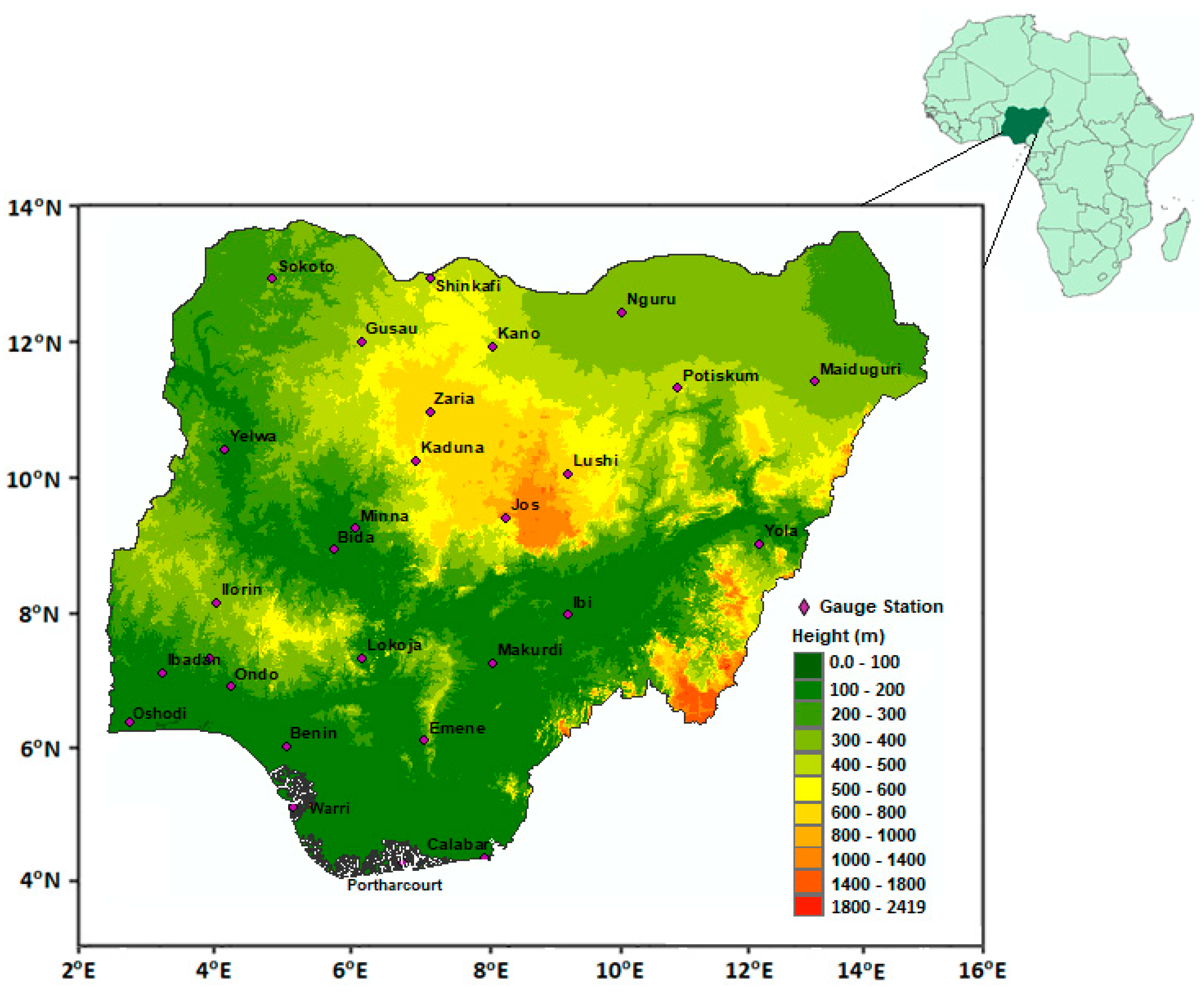
The area of study, Nigeria, is located in Western Africa between Latitudes 4°15′–13°55′ N; Longitude: 2°40′ and 14°45′ E 923,000 km2 area (Figure 1). The seasons in Nigeria are divided into the wet (rainy) and the dry. The country receives more than 2000 mm rainfall in the southern region starting in April and ending in October. The northernmost parts receive rainfalls below 500 mm which mostly occur in June to September. Temperatures during the dry season range between 30° to 37 °C in the south while temperatures in the north are higher and can reach as high as 45 °C in the northeastern and northwestern parts. The harmattan season, which occurs between December and February in the dry season, has the lowest records of temperatures in Nigeria. During this season, temperatures range from 17–24 °C in the south and can reach lows of 12 °C in the north.
The ecology of Nigeria varies from the north to the south. The northern part has the Sahel and Sudan savanna type ecology, the central has the Guinea savanna type while the Mangrove swamp is in the southernmost part of the country. This can be attributed to variation in the climatic condition of the country with warm desert and semi-arid climate in the north, the tropical savanna climate in the center, and the monsoon climate in the south. Elevation within the country ranges from 0 m at the Atlantic Ocean coast in the south to 2419 m at Chappal Waddi in the north.
2.2. Data
2.2.1. Historical Rainfall Data
This study made use of the GPCC full data reanalysis rainfall product of the Deutscher Wetterdienst [38] as the data of reference. The GPCC precipitation product amongst most similar products offers the following advantages: (1) good quality of data for climate studies, (2) long time data span for wider study period, (3) produced based on the highest number of precipitation record, (4) time series completeness after January 1951 [39,40]. This study uses the monthly precipitation data between the periods of 1961–2005 at 323 grid points over Nigeria.
2.2.2. CMIP5 Datasets
Historical and future simulations of the CMIP5 GCMs available from different modeling groups under the Assessment Report (AR5) was used in this study [41]. The CMIP5 has significant improvements over the previous CMIP3 offering larger number of models of higher resolutions and improvements in models’ physics [41,42]. This study made a selection of 20 monthly rainfall GCMs simulations of the CMIP5 for Nigeria based on RCPs (4.5 and 8.5) availability for the country. The rainfall GCMs’ selected, their resolutions and the centers of modeling are presented in Table 1.
3. Methods
3.1. Bias Correction of GCMs
BC is the correction of biases involving the feeding of local climatic information into GCMs [43]. There are various BC methods including analog methods [44], multiple linear regression [2], delta change method [45], monthly mean correction [46], gamma–gamma transformation [47], quantile mapping [48], fitted histogram equalization [49], and scaling method [50]. The four methods that were used in this study are discussed as follows. These four BC methods were selected based on their wide applicability in correction of GCM rainfall biases.
3.1.1. Gamma Quantile Mapping (GAQM)
GAQM [49] has its basis on the assumption that the observed and simulated intensity distributions are well approximated by a gamma distribution. A model variable is built by GAQM using probability integral transform in a manner that the distribution that is newly built becomes equal to the distribution of the observed variable .
where, = Cumulative function of , and = inverse cumulative function of . The probability density function (PDF) of gamma distribution is defined as follows:
where, x = Normalized daily precipitation; k = Form parameter; and θ = Scaling parameter.
In GAQM, the value of k is assumed >1 because if k = 0 (exponential distribution) or k < 1 (dry months), therefore when k = 0 or k = 1 GAQM cannot be applied.
3.1.2. General Quantile Mapping (GEQM)
GEQM [51] is a form of parametric quantile mapping. The main difference is that in GEQM, gamma distribution and Generalized Pareto Distribution (GPD) are applied. The general equation of GEQM is given below.
However, in this equation, the pdf is replaced with the gamma distribution and GPD. GPD is heavily tailed with extreme value distribution [46].
where is a threshold given by the 95th percentile value, in which is the scale parameter whereas, is the shape parameter. In this method the gamma distribution is applied on smaller threshold (values less then 95th percentile) and GPD is applied on values larger than this threshold.
where and are the cumulative density functions for the gamma and GPD distributions, respectively.
3.1.3. Power Transformation (PT)
The bias in the mean as well as the variance differences for the correction of data is considered by the PT [52]. In the method, a non-linear correction in the exponential form such as can be applied in adjusting the variance. In this method, rainfall is changed to a corrected amount of using the expression below.
Parameter b is calculated by a distribution-free approach, in which b is firstly identified through matching of the coefficient of variation (CV) corrected daily rainfall () with that of the observed daily rainfall for the training period. The b value is iteratively determined. The data are grouped into every 5-day periods of the year to reduce the sampling variability [53]. Using the value of b, the transformed rainfall is calculated with
The parameter a has its basis on the mean of the observed and the mean of the transformed values. Parameter a is dependent upon b, and b is dependent upon CV. The values of a and b are different for every 5-day block of each year.
3.1.4. Linear Scaling (LS)
LS [54] uses the monthly correction values which are calculated by the difference in observed and simulated daily data. The monthly scaling factor is used for the uncorrected daily data. The daily rainfall P is corrected by the following equation.
For the BC of rainfall, the scaling factor is calculated by
is the observed rainfall mean whereas is the monthly mean of the simulated rainfall. LS method is simple and requires less information such as only monthly data for calculation of the scaling factor [55].
3.2. Performance Assessment of Bias Correction (BC) Methods
The performances of the BC methods in downscaling GCM rainfall at the GPCC grid points over Nigeria were assessed using statistical metrics namely, relative standard deviation (RSD), percentage of bias (Pbias), normalized root mean square (NRMSE), Nash-Sutcliffe efficiency (NSE), modified index of agreement (MD) and volumetric efficiency (Ve) during the validation period (1993–2005). This was able to show the individual contributions of the different GCMs to the uncertainties in the MME mean rainfall from each of the BC methods. The PDFs of the individual models were used for the assessment of the ability of the different GCMs to replicate the historical rainfall using the different BC methods.
3.3. Ensemble Projections
MMEs based on regression can preserve the variance in its average and has been widely applied in recent times. Multiple linear regressions however have no ability of explicating the nonlinear relationship existing between the dependent and the independent variables, even when significance is in their relationship. However, RF has that ability of explicating the regression coefficient [56] and has been applied in this study for the conversion of the selected rainfall GCMs into an ensemble.
RF has many advantages of being effective and robust in generating MMEs including (1) avoiding over-fitting, (2) possible implementation of different types of input variables without need for deleting any or regularization and (3) flexibility in its analysis and operations. Therefore, the building of regression models for precipitation relating to a number of predictors covering different spatial scales is possible in this study. The projection of rainfall during 2010–2039, 2040–2069 and 2070–2099 analyzed against the historical period 1971–2000 for Nigeria was estimated using the average variances of the MME rainfalls of the different BC methods. The best performing BC method was selected for the spatial projection of rainfall in the study area.
4. Results
4.1. Performance Evaluation of Bias Corrected Models
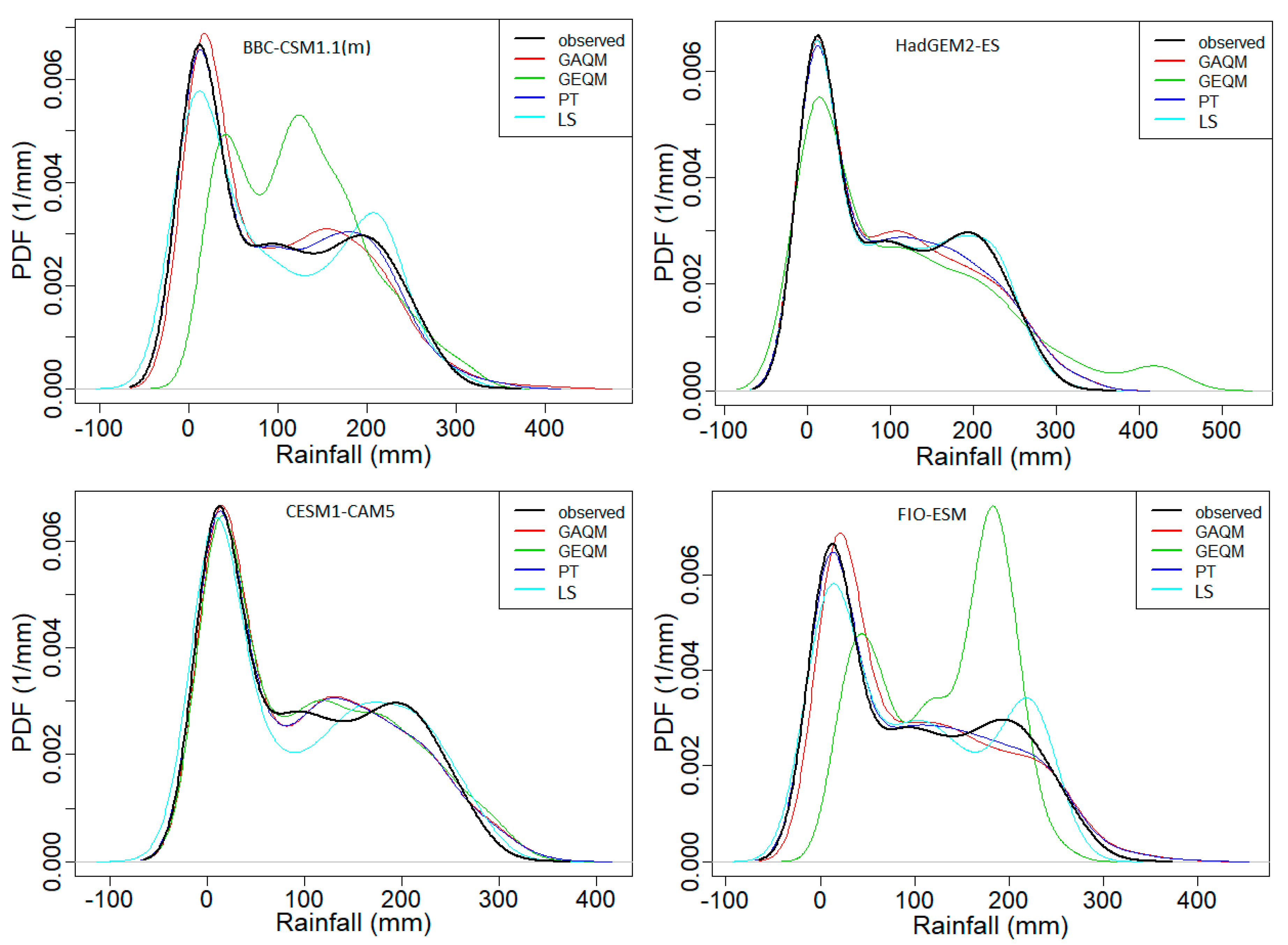
The results of the performances of the downscaling models for the four BC methods used in this study are presented in Figure 2 for some of the GCMs used in this study (Table 1). The comparisons show that there are variations in the performances of the downscaling models depending on the GCM and the BC methods. For example, while the GEQM BC method was able to reproduce the properties of the observed rainfall for the GCMs CESM1-CAM5, the method had lesser performance to reproduce the properties for the GCMs BBC-CSM1.1 (m) and FIO-ESM. The PDFs showed that the PT BC method was able to replicate the rainfall best followed by the LS and the GAQM methods.
4.2. Performance Assessment of Bias Correction Methods
The averages of the performances of the twenty GCMs for the different BC methods using six statistical indices are presented in Table 2. The LS method generally performed better in bias correcting the models as compared to the other methods. The PT and the GAQM have close performances while the GEQM was the least performing of all methods.
For assessment of the efficiency of the LS method, which was the best performing BC method in the correction of the biases in the GCMs as seen in Table 2, scatter plot was used. The scatter plots for some of the GCMs are presented in Figure 3. There are stronger relations between the bias corrected rainfalls and the observed, compared to the rainfall of raw GCMs as seen in the figure.
4.3. Rainfall Projection
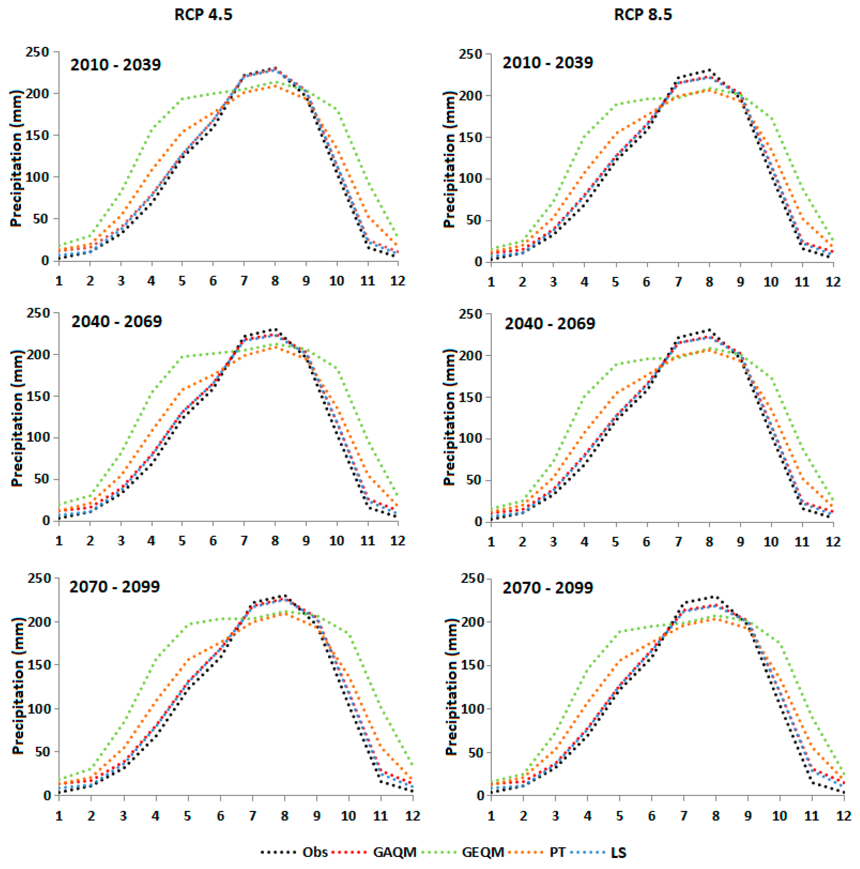
The mean monthly changes in projected rainfall for the MMEs of GCMs using the four BC methods were compared to the observed GPCC rainfall (1971–2000) as shown in Figure 4. The projection of rainfall was performed for the different periods of 2010–2039, 2040–2069 and 2070–2099 for RCPs 4.5 and 8.5. The figure shows that during the period 2010–2039, rainfall increased in the dry season, November to after April, with the least increments for the MMEs of the LS and the GAQM for both RCPs 4.5 and 8.5. In the same period, the results of GEQM shows the highest increments and it was followed by the PT method. However, during the wet season (June–September), the GEQM and the PT MMEs projected decrease in rainfall up to about 20 mm. While there were no changes in rainfall during this period (2010–2039) under RCP 4.5 for the LS and the GAQM MMEs, there were projections of decrease under RCP 8.5. The projections during the periods 2040–2069 and 2070–2099 showed that there would be more decrease in rainfall for the wet season compared to the period 2010–2039. The highest decreases in rainfall are projected for 2070–2099 under RCP 8.5.
The mean annual wet season (June–September) rainfalls (mm) for the future periods under RCPs 4.5 and 8.5 for the different BC methods are presented in Figure 5. The figure shows that the least mean monthly rainfall expected in the future over Nigeria was estimated by the PT BC method. This will occur during 2070–2099 under RCP 8.5. In comparison to the other methods, the GEQM method gave the highest estimate of the mean monthly rainfall over the country. From the method, the rainfall will be the highest under RCP 4.5 during 2040–2069. Estimation of the monthly mean rainfall for the GAQM and the LS were observed to be similar for both RCPs and for the three periods.
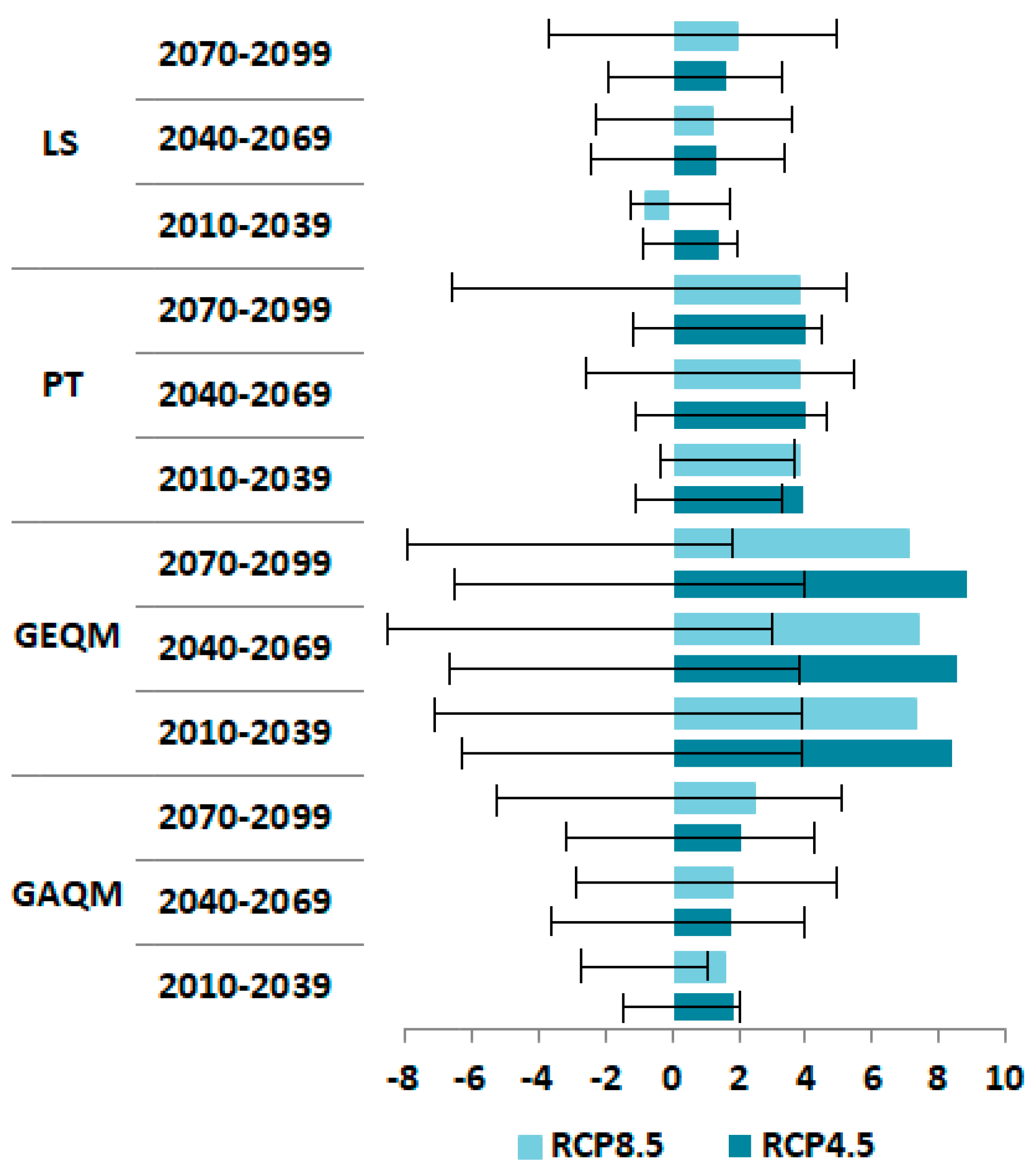
The percentage changes in projected annual rainfall under RCPs 4.5 and 8.5 for the different BC methods referenced to the base rainfall (GPCC) (1971–2000) were compared and results presented in Figure 6. For estimation of the changes in rainfall, the average of the GPCC rainfall during 1971–2000, 323 grid points were subtracted from those of the projected rainfalls for the future periods, 2010–2039, 2040–2069 and 2070–2099 for the four BC methods. The expected changes in future rainfall and the levels of uncertainty were estimated using the MME mean from the different BC methods and its 95% confidence band. The highest percentage changes in rainfall were projected by the GEQM method followed by the PT method. The LS and the GAQM methods have almost the same percentages of changes in rainfall in the future. There are variations in uncertainties among the BC methods, the periods and between the RCPs. Uncertainty was highest for the GEQM method during 2040–2069 period. The least uncertainty was observed for the LS method under RCP 8.5 during 2010–2039. Uncertainties in the rainfall projection were generally higher under RCP 8.5 than under RCP 4.5.
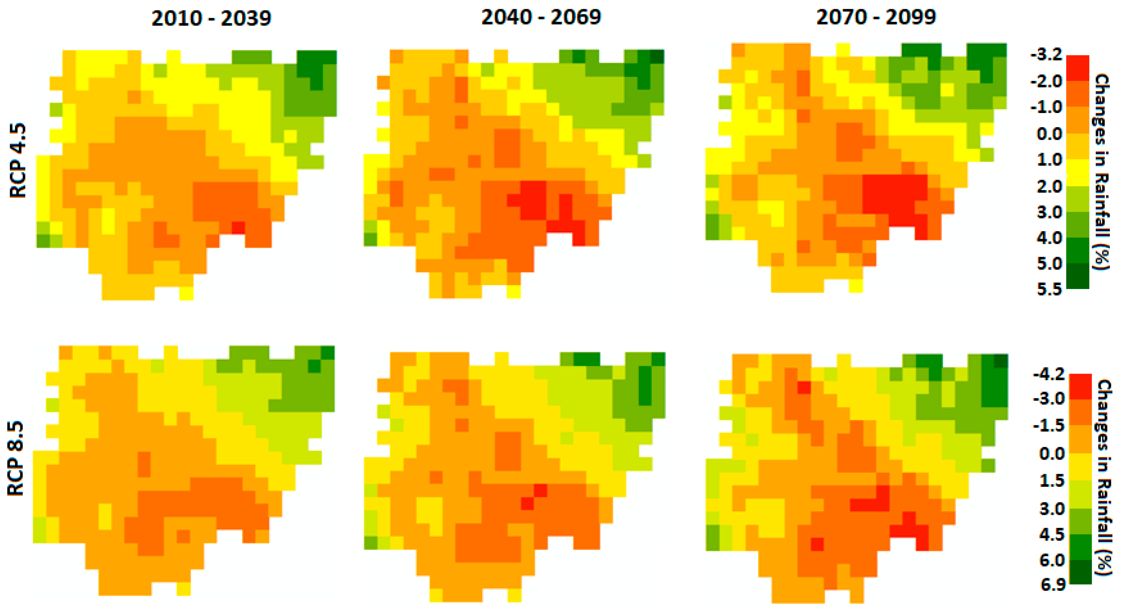
4.3.1. Spatial Changes in Wet Season Rainfall for LS
The spatial patterns of the changes (in percentage) of the mean annual wet season rainfall for the periods 2010–2039, 2040–2069 and 2070–2099 for the MME of the LS method are presented in Figure 7 for RCP 4.5 and 8.5. Figure shows for RCP 4.5, rainfall will decrease by up to −3.2% mostly in the south east and central parts of the country. Rainfall is expected to increase at the northeast of the country under this RCP by up to 5.5%. Projections under RCP 8.5 show that increases in rainfall are expected in the north east of the country up to 6.9% while rainfalls will decrease by up to 4.2% also mostly at the south east of the country.
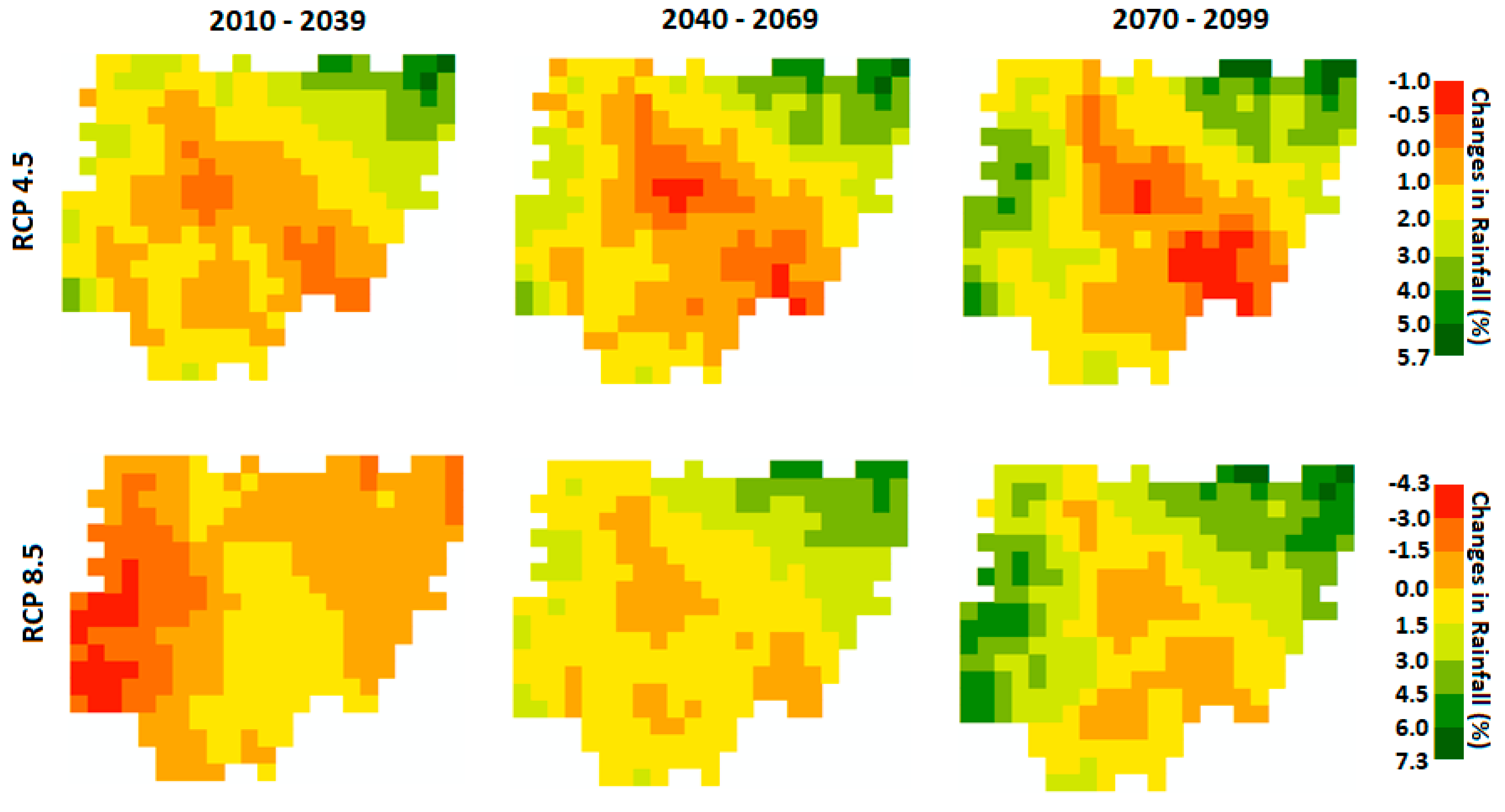
4.3.2. Spatial Changes in Annual Rainfall
The spatial patterns of the changes (in percentage) of the mean annual rainfall for the periods 2010–2039, 2040–2069 and 2070–2099 for the MME of the LS method are presented in Figure 8 for RCP 4.5 and 8.5. For the annual projections under RCP4.5, the expected increases in rainfall are up to 5.7%. Under RCP 8.5, rainfall decreases are expected to occur at lesser areas during 2040–2069 and 2070–2099 compared to the RCP 4.5. However, decreases are expected to be higher at the south west parts of the country compared to RCP4.5 during 2010–2039.
5. Discussion
Lesser than usual rainfall can significantly affect several sectors including energy, agriculture, water resources and industrial, which subsequently have debilitating impacts on the socio-economic and environmental aspects. Many studies have shown the risks of possible droughts that could arise from decreases in rainfall in some parts and risk of increasing flood as a result of increasing rainfall in other parts. Manawi et al. [57] reported the risks posed by flooding in the urban areas of northern Kabul city, Afghanistan, due to excessive precipitation during the monsoon seasons. Flood events were reported in many parts of West Africa due to above normal precipitation during June–September compared to the last 35 years due to an overall increase in the intensity of rainfall during the monsoon season [58]. Homsi et al. [59] showed that there would be a decrease of annual rainfall in the range of −30–−85% over Syria under all RCPs during the wet seasons. During the dry season, the decreases are expected to be −12–−93%, indicating drier conditions for the country. Sa’adi et al. [22] projected the spatial temporal changes of rainfall in the Sarawak area of Borneo Island using the CMIP5 GCMs. The study revealed both increases and decreases in mean annual rainfall in the study area. The CMIP5 was used in the United States for projection and identification of spatial hotspots of precipitation changes [60]. The study revealed there are region-specific hotspots of future changes in precipitation and larger changes should be expected under RCP 8.5 than under RCP 4.5 during 2040–2095. In South America, Palomino-Lemus et al. [61] projected precipitation using CMIP5, and the study showed that as the radiative forcing increases from RCP2.6–8.5, the changes in rainfall range from moderate (±25%) to intense (from ±70% to ±100%). Droughts have also been projected to increase in some parts of the globe under the CMIP5 GCMs [62,63]
In Africa, Obuobie et al. [64] analyzed the changes in downscaled rainfall over the Volta River Basin of West Africa and found that annual rainfall is expected to increase by between 3–4% and 3–5% at all the three climatic zones within the basin under the A1B and A2 scenarios, respectively. In Nigeria, Abiodun et al. [65] under emission scenarios B1 and A2 assessed the possible global warming impacts on future climate and extreme events on the future climates for the period 2046–2065 and 2081–2100. The study showed increases in temperature should be expected at all ecological zones of the country. These changes may aggravate extreme rainfall events and their frequencies in the southeast and the south, and there may be annual reduction in rainfall in the northeast causing floods and droughts, respectively. Though this present study corroborates some of the findings from their study, it does not support expected increase in rainfall in the southeast of the country. Rather, rainfall is expected to decrease in the south east of the country. The northeast, where the study reported expected decreases in rainfall, is projected in this present study to have increased rainfall except for the average annual projection under RCP8.5 during 2010–2039. This difference in the findings can probably be attributed to the GCM data applied in the studies. The expected decrease in rainfall, particularly in the central parts of the country, which constitutes the major contributor to agricultural production and projected temperature increases [24] in the country, will have significant impacts on the area and the country at large.
Although, improvements of climate models, e.g., of CMIP5 have been reported [41], climate projections even with such models are characterized by uncertainties originating from various sources including those arising from exclusive sources like different emission/concentration scenarios, parameterization and GCMs’ structures, and boundary and initial conditions [66,67]. In addition, studies have found that the BC method of downscaling used for the removal of bias in GCMs can be an additional uncertainty source in any resulting climate ensemble [25,26]. The methodology and data applied in this study were carefully evaluated in the projections of the climate for the study area. The quantification of uncertainties relating to data used was not assessed in this study as they are inherent, such as in GCMs, during their preparations [68]. The projections from the best performing BC method can be a guide to the possible expected changes in precipitation and their impacts on disasters risks evaluation. Furthermore, evaluations such as comparing results presented here to those from future studies such as those using of the CMIP6 are crucial.
6. Conclusions
This study compares the rainfall projections from MMEs of 20 GCMs for four BC methods: GAQM, GEQM, PT and LS. The rainfall projections were conducted for Nigeria during 2010–2039, 2040–2069 and 2070–2099 for RCPs 4.5 and 8.5. The study uses the GPCC data of the historical period 1961–2005 and the historical and the future simulations of the GCMs of the CMIP5. The performances of the different BC methods in removing biases from the GCMs were assessed using different statistical indices. The computation of the MME mean of the projected rainfall was conducted using the random forest regression method. The spatial distributions of projected rainfall using the best performing BC method were conducted for RCP4.5 and 8.5 for the aforementioned three periods.
The study revealed that of the four BC methods, the LS method was the best in removing the biases from the GCMs. The spatial distributions of rainfall using the MME of LS method show that the southeast down to the south–south part of the country will experience decrease in rainfall. In the northeast part of the country, rainfalls are expected to increase according to the spatial projections from the LS BC method. The monthly rainfall within the country will decrease during the wet season between June and September, which is a significant period where most crops needs the water for growth.
This study has demonstrated that while some parts of Nigeria will experience an increase in rainfall in the future, other parts are expected to experience decreases. Most populace of the rural areas are dependent on rainfall agriculture, which is their primary source of income. The decrease in future rainfall in some areas, particularly the central and some southern parts of the country where agriculture is extensively practiced, jeopardizes their source of income and food security in the country. It is anticipated that the outcomes of this study can be a guide in the development of adaptation and mitigation measures for the country in combating the menace of climate change.
Author Contributions
Conceptualization, M.S.S.; methodology, M.S.S.; software, M.S.S.; validation, M.S.S.; writing—original draft preparation, M.S.S.; writing—review and editing, M.S.S. and I.P.; project administration, I.P.; funding acquisition, I.P. All authors have read and agreed to the published version of the manuscript.
Funding
This research was funded by Seoul National University of Science and Technology.
Acknowledgments
This study was financially supported by Seoul National University of Science and Technology.
Conflicts of Interest
The authors declare no conflict of interest.
References
- Alamgir, M.; Mohsenipour, M.; Homsi, R.; Wang, X.; Shahid, S.; Shiru, M.S.; Alias, N.E.; Yuzir, A. Parametric Assessment of Seasonal Drought Risk to Crop Production in Bangladesh. Sustainability 2019, 11, 1442. [Google Scholar] [CrossRef] [Green Version]
- Hay, L.E.; Clark, M. Use of statistically and dynamically downscaled atmospheric model output for hydrologic simulations in three mountainous basins in the western United States. J. Hydrol. 2003, 282, 56–75. [Google Scholar] [CrossRef]
- Salman, S.A.; Shahid, S.; Afan, H.A.; Shiru, M.S.; Al-Ansari, N.; Yaseen, Z.M. Changes in Climatic Water Availability and Crop Water Demand for Iraq Region. Sustainability 2020, 12, 3437. [Google Scholar] [CrossRef] [Green Version]
- Sylla, M.B.; Elguindi, N.; Giorgi, F.; Wisser, D. Projected robust shift of climate zones over West Africa in response to anthropogenic climate change for the late 21st century. Clim. Chang. 2016, 134, 241–253. [Google Scholar] [CrossRef]
- Westra, S.; Alexander, L.V.; Zwiers, F.W. Global increasing trends in annual maximum daily precipitation. J. Clim. 2012, 26, 3904–3918. [Google Scholar] [CrossRef] [Green Version]
- Rudd, A.C.; Kay, A.L.; Wells, S.C.; Aldridge, T.; Cole, S.J.; Kendon, E.J.; Stewart, E.J. Investigating potential future changes in surface water flooding hazard and impact. Hydrol. Process. 2020, 34, 139–149. [Google Scholar]
- Sa’adi, Z.; Shiru, M.S.; Shahid, S.; Ismail, T. Selection of general circulation models for the projections of spatio-temporal changes in temperature of Borneo Island based on CMIP5. Theor. Appl. Clim. 2019, 139, 351–371. [Google Scholar] [CrossRef]
- Ahmed, K.; Iqbal, Z.; Khan, N.; Rasheed, B.; Nawaz, N.; Malik, I.; Noor, M. Quantitative assessment of precipitation changes under CMIP5 RCP scenarios over the northern sub-Himalayan region of Pakistan. Environ. Dev. Sustain. 2019, 1–15. [Google Scholar] [CrossRef]
- Khan, N.; Shahid, S.; Ahmed, K.; Wang, X.; Ali, R.; Ismail, T.; Nawaz, N. Selection of GCMs for the projection of spatial distribution of heat waves in Pakistan. Atmos. Res. 2020, 233, 104688. [Google Scholar] [CrossRef]
- Van Huijgevoort, M.; Van Lanen, H.; Teuling, A.; Uijlenhoet, R. Identification of changes in hydrological drought characteristics from a multi-GCM driven ensemble constrained by observed discharge. J. Hydrol. 2014, 512, 421–434. [Google Scholar] [CrossRef] [Green Version]
- Naumann, G.; Alfieri, L.; Wyser, K.; Mentaschi, L.; Betts, R.; Carrao, H.; Spinoni, J.; Feyen, L. Global changes in drought conditions under different levels of warming. Geophys. Res. Lett. 2018, 45, 3285–3296. [Google Scholar] [CrossRef]
- Dikshit, A.; Pradhan, B.; Alamri, A.M. Pathways and challenges of the application of artificial intelligence to geohazards modelling. Gondwana Res. 2020, in press. [Google Scholar] [CrossRef]
- Khan, N.; Sachindra, D.; Shahid, S.; Ahmed, K.; Shiru, M.S.; Nawaz, N. Prediction of droughts over Pakistan using machine learning algorithms. Adv. Water Resour. 2020, 139, 103562. [Google Scholar] [CrossRef]
- Fowler, H.J.; Blenkinsop, S.; Tebaldi, C. Linking climate change modelling to impacts studies: Recent advances in downscaling techniques for hydrological modelling. Int. J. Climatol. 2007, 27, 1547–1578. [Google Scholar] [CrossRef]
- Rashid, M.M.; Beecham, S.; Chowdhury, R.K. Statistical downscaling of CMIP5 outputs for projecting future changes in rainfall in the Onkaparinga catchment. Sci. Total Environ. 2015, 171–182. [Google Scholar] [CrossRef] [PubMed]
- Hundecha, Y.; Sunyer, M.A.; Lawrence, D.; Madsen, H.; Willems, P.; Bürger, G.; Kriaucˇiuniene, J.; Loukas, A.; Martinkove, M.; Osuch, M.; et al. Inter-comparison of statistical downscaling methods for projection of extreme flow indices across Europe. J. Hydrol. 2016, 541, 1273–1286. [Google Scholar] [CrossRef]
- Wang, B.; Zheng, L.; Liu, D.L.; Ji, F.; Clark, A.; Yu, Q. Using multi-model ensembles of CMIP5 global climate models to reproduce observed monthly rainfall and temperature with machine learning methods in Australia. Int. J. Climatol. 2018, 38, 4891–4902. [Google Scholar] [CrossRef]
- Salman, S.A.; Shahid, S.; Ismail, T.; Ahmed, K.; Wang, X.-J. Selection of climate models for projection of spatiotemporal changes in temperature of Iraq with uncertainties. Atmos. Res. 2018, 213, 509–522. [Google Scholar] [CrossRef]
- Chen, J.; Brissette, F.P.; Lucas-Picher, P.; Caya, D. Impacts of weighting climate models for hydro-meteorological climate change studies. J. Hydrol. 2017, 549, 534–546. [Google Scholar] [CrossRef]
- Brown, J.D.; Seo, D.J. Evaluation of a nonparametric post-processor for bias correction and uncertainty estimation of hydrologic predictions. Hydrol. Process. 2013, 27, 83–105. [Google Scholar] [CrossRef]
- Gaborit, É.; Anctil, F.; Fortin, V.; Pelletier, G. On the reliability of spatially disaggregated global ensemble rainfall forecasts. Hydrol. Process. 2013, 27, 45–56. [Google Scholar] [CrossRef]
- Sa’adi, Z.; Shahid, S.; Chung, E.S.; Ismail, T. Projection of spatial and temporal changes of rainfall in Sarawak of Borneo Island using statistical downscaling of CMIP5 models. Atmos. Res. 2017, 197, 446–460. [Google Scholar] [CrossRef]
- Khan, N.; Shahid, S.; Ahmed, K.; Ismail, T.; Nawaz, N.; Son, M. Performance assessment of general circulation model in simulating daily precipitation and temperature using multiple gridded datasets. Water 2018, 10, 1793. [Google Scholar] [CrossRef] [Green Version]
- Shiru, M.S.; Chung, E.-S.; Shahid, S.; Alias, N. GCM selection and temperature projection of Nigeria under different RCPs of the CMIP5 GCMS. Theor. Appl. Climatol. 2020, 141, 1611–1627. [Google Scholar] [CrossRef]
- Akstinas, V.; Jakimavicius, D.; Meilutyte-Lukauskiene, D.; Kriauciuniene, J.; Sarauskiene, D. Uncertainty of annual runoff projections in Lithuanian rivers under a future climate. Hydrol. Res. 2020, 51, 257–271. [Google Scholar] [CrossRef]
- Wooten, A.; Terando, A.; Reich, B.J.; Boyles, R.P.; Semazzi, F. Characterizing Sources of Uncertainty from Global Climate Models and Downscaling Techniques. J. Appl. Meteorol. Climatol. 2017, 56, 3245–3262. [Google Scholar] [CrossRef]
- Sharma, T.; Vittal, H.; Chhabra, S.; Salvi, K.; Ghosh, S.; Karmakar, S. Understanding the cascade of GCM and downscaling uncertainties in hydro-climatic projections over India. Int. J. Climatol. 2018, 38, 178–190. [Google Scholar] [CrossRef]
- Medugu, N.I.; Majid, M.R.; Johar, F. Drought and desertification management in arid and semi-arid zones of Northern Nigeria. Manag. Environ. Qual. Int. J. 2011, 22, 595–611. [Google Scholar] [CrossRef]
- Usman, M.T.; Abdulkadir, A. Review: An experiment in intra-seasonal agricultural drought monitoring and early warning in the Sudano-Sahelian Belt of Nigeria. Int. J. Climatol. 2014, 34, 2129–2135. [Google Scholar] [CrossRef]
- Oloruntade, A.J.; Mohammad, T.A.; Ghazali, A.H.; Wayayok, A. Analysis of meteorological and hydrological droughts in the Niger-South Basin, Nigeria. Glob. Planet. Chang. 2017, 155, 225–233. [Google Scholar] [CrossRef]
- Shiru, M.S.; Shahid, S.; Alias, N.; Chung, E.-S. Trend Analysis of Droughts during Crop Growing Seasons of Nigeria. Sustainability 2018, 10, 871. [Google Scholar] [CrossRef] [Green Version]
- Douglas, I.; Alam, K.; Maghenda, M.; McDonnel, Y.; McLean, L.; Campbell, J. Unjust waters: Climate change, flooding and the urban poor in Africa. Environ. Urban. 2008, 20, 187–205. [Google Scholar] [CrossRef] [Green Version]
- National Emergency Management Agency (NEMA). Worst Flooding in Decades. Available online: http://reliefweb.int/report/nigeria/worst-flooding-decades (accessed on 6 April 2020).
- Macdonald, A.M.; Cobbing, J.; Davies, J. Developing Groundwater for Rural Water Supply in Nigeria: A Report of the May 2005 Training Course and Summary of the Groundwater Issues in the Eight Focus States; British Geological Survey Commissioned Report, CR/05/219N; ITDG: Bradford, UK, 2005; p. 32. [Google Scholar]
- Adelana, S.M.A.; Olasehinde, P.I.; Vrbka, P. A quantitative estimation of groundwater recharge in part of the sokoto basin, Nigeria. J. Environ. Hydrol. 2006, 14, 1–14. [Google Scholar]
- Shiru, M.S.; Shahid, S.; Chung, E.-S.; Alias, N. Changing characteristics of meteorological droughts in Nigeria during 1901–2010. Atmos. Res. 2019, 223, 60–73. [Google Scholar] [CrossRef]
- World Bank Group. Agriculture, Value Added (% of GDP). Available online: http://data.worldbank.org/indicator/NV.AGR.TOTL.ZS (accessed on 18 April 2020).
- Becker, A.; Finger, P.; Meyer-Christoffer, A.; Rudolf, B.; Schamm, K.; Schneider, U.; Ziese, M. A description of the global land-surface precipitation data products of the global precipitation climatology Centre with sample applications including centennial (trend) analysis from 1901-present. Earth Syst. Sci. 2013, 5, 71–99. [Google Scholar] [CrossRef] [Green Version]
- Spinoni, J.; Naumann, G.; Carrao, H.; Barbosa, P.; Vogt, J. World drought frequency, duration, and severity for 1951–2010. Int. J. Clim. 2014, 34, 2792–2804. [Google Scholar] [CrossRef] [Green Version]
- Ahmed, K.; Shahid, S.; Chung, E.-S.; Ismail, T.; Wang, X.-J. Spatial distribution of secular trends in annual and seasonal precipitation over Pakistan. Clim. Res. 2017, 74, 95–107. [Google Scholar] [CrossRef]
- Taylor, K.E.; Stouffer, R.J.; Meehl, G.A. An overview of CMIP5 and the experiment design. Bull. Am. Meteorol. Soc. 2012, 93, 485–498. [Google Scholar] [CrossRef] [Green Version]
- Knutti, R.; Sedlácek, J. Robustness and uncertainties in the new CMIP5 climate model projections. Nat. Clim. Change 2013, 3, 369–373. [Google Scholar] [CrossRef]
- Akhter, J.; Das, L.; Deb, A. CMIP5 ensemble-based spatial rainfall projection over homogeneous zones of India. Clim. Dyn. 2017, 49, 1885–1916. [Google Scholar] [CrossRef]
- Moron, V.; Robertson, A.W.; Ward, M.N.; Ndiaye, O. Weather types and rainfall over Senegal, Part II: Downscaling of GCM simulations. J. Clim. 2008, 21, 288–307. [Google Scholar] [CrossRef]
- Hay, L.E.; Wilby, R.J.L.; Leavesley, G.H. A comparison of delta change and downscaled GCM scenarios for three mountainous basins in the United States. J. Am. Water Resour. Assoc. 2000, 36, 387–397. [Google Scholar] [CrossRef]
- Fowler, H.; Kilsby, C. Using regional climate model data to simulate historical and future river flows in northwest England. Clim. Chang. 2007, 80, 337–367. [Google Scholar] [CrossRef]
- Sharma, D.; Das Gupta, A.; Babel, M.S. Spatial disaggregation of bias-corrected GCM precipitation for improved hydrologic simulation: Ping River Basin, Thailand. Hydrol. Earth Syst. Sci. 2007, 11, 1373–1390. [Google Scholar] [CrossRef] [Green Version]
- Wood, A.W.; Leung, L.R.; Sridhar, V.; Lettenmaier, D.P. Hydrologic implications of dynamical and statistical approaches to downscaling climate model outputs. Clim. Chang. 2004, 62, 189–216. [Google Scholar] [CrossRef]
- Piani, C.; Weedon, G.P.; Best, M.; Gomes, S.M.; Viterbo, P.; Hagemann, S.; Haerter, J.O. Statistical bias correction of global simulated daily precipitation and temperature for the application of hydrological models. J. Hydrol. 2010, 395, 199–215. [Google Scholar] [CrossRef]
- Mahmood, R.; JIA, S. An extended linear scaling method for downscaling temperature and its implication in the Jhelum River basin, Pakistan, and India, using CMIP5 GCMs. Theor. Appl. Climatol. 2017, 130, 725–734. [Google Scholar] [CrossRef]
- Coles, S. An Introduction to Statistical Modelling of Extreme Values; Springer: Berlin/Heidelberg, Germany, 2001. [Google Scholar]
- Leander, R.; Buishand, T.A. Resampling of regional climate model output for the simulation of extreme river flows. J. Hydrol. 2007, 332, 487–496. [Google Scholar] [CrossRef]
- Terink, W.; Hurkmans, R.T.W.L.; Torfs, P.J.J.F.; Uijlenhoet, R. Bias correction of temperature and precipitation data for regional climate model application to the Rhine basin. Hydrol. Earth Syst. Sci. Discuss. 2009, 6, 5377–5413. [Google Scholar] [CrossRef] [Green Version]
- Lenderink, G.; van Ulden, A.; van den Hurk, B.; Keller, F. A study on combining global and regional climate model results for generating climate scenarios of temperature and precipitation for the Netherlands. Clim. Dyn. 2007, 29, 157–176. [Google Scholar] [CrossRef] [Green Version]
- Lafon, T.; Dadson, S.; Buys, G.; Prudhomme, C. Bias correction of daily precipitation simulated by a regional climate model: A comparison of methods. Int. J. Climatol. 2013, 33, 1367–1381. [Google Scholar] [CrossRef] [Green Version]
- Li, J.; Heap, A.D.; Potter, A.; Daniell, J.J. Application of machine learning methods to spatial interpolation of environmental variables. Environ. Model. Softw. 2011, 26, 1647–1659. [Google Scholar] [CrossRef]
- Manawi, S.M.A.; Nasir, K.A.M.; Shiru, M.S.; Hotaki, S.F.; Sediqi, M.N. Urban Flooding in the Northern Part of Kabul City: Causes and Mitigation. Earth Sys. Environ. 2020, 4, 569–610. [Google Scholar] [CrossRef]
- Adegoke, J.; Sylla, M.B.; Taylor, C.; Klein, C.; Bossa, A.; Kehinde Ogunjobi, K.; Adounkpe, J. On the 2017 Rainy Season Intensity and Subsequent Flood Events over West Africa. In Regional Climate Change Series: Floods; WASCAL: Accra, Ghana, 2019; pp. 10–15. [Google Scholar]
- Homsi, R.; Shiru, M.S.; Shahid, S.; Ismail, T.; Harun, S.; Al-Ansari, N.; Chau, K.-W.; Yaseen, Z.M. Precipitation projection using a CMIP5 GCM ensemble model: A regional investigation of Syria. Eng. Appl. Comput. Fluid Mech. 2020, 14, 90–106. [Google Scholar] [CrossRef]
- Jiang, M.; Felzer, B.S.; Sahagian, D. Predictability of precipitation over the conterminous US based on the CMIP5 multi-model ensemble. Sci. Rep. 2016, 6, 1–9. [Google Scholar]
- Palomino-Lemus, R.; Córdoba-Machado, S.; Gámiz-Fortis, S.R.; Castro-Díez, Y.; Esteban-Parra, M.J. Climate change projections of boreal summer precipitation over tropical America by using statistical downscaling from CMIP5 models. Environ. Res. Lett. 2017, 12, 124011. [Google Scholar] [CrossRef] [Green Version]
- Ruosteenoja, K.; Markkanen, T.; Venäläinen, A.; Räisänen, P.; Peltola, H. Seasonal soil moisture and drought occurrence in Europe in CMIP5 projections for the 21st century. Clim. Dyn. 2018, 50, 1177–1192. [Google Scholar] [CrossRef] [Green Version]
- Shiru, M.S.; Shahid, S.; Dewan, A.; Chung, E.-S.; Alias, N.; Ahmed, K.; Hassan, Q.K. Projection of meteorological droughts in Nigeria during growing seasons under climate change scenarios. Sci. Rep. 2020, 10, 1–18. [Google Scholar] [CrossRef]
- Obuobie, E.; Amisigo, B.; Logah, F.; Kankam-Yeboah, K. Analysis of changes in downscaled rainfall and temperature projections in the Volta River Basin. In Dams, Development and Downstream Communities: Implications for Re-Optimising the Operations of the Akosombo and Kpong Dams in Ghana; Ntiamoa-Baidu, Y., Ampomah, B.Y., Ofosu, E.A., Eds.; Digibooks Gh. Ltd.: Tema, Ghana, 2017. [Google Scholar]
- Abiodun, B.J.; Lawal, K.A.; Salami, A.T.; Abatan, A.A. Potential influences of global warming on future climate and extreme events in Nigeria. Reg. Environ. Chang. 2013, 13, 477–491. [Google Scholar] [CrossRef]
- Brekke, L.; Barsugli, J. Uncertainties in projections of future changes in extremes. In Extremes in a Changing Climate: Detection, Analysis and Uncertainty; AghaKouchak, A., Easterling, D., Hsu, K., Schubert, S., Sorooshian, S., Eds.; Springer: Berlin/Heidelberg, Germany, 2013; pp. 309–346. [Google Scholar]
- Strobach, E.; Bel, G. The contribution of internal and model variabilities to the uncertainty in CMIP5 decadal climate predictions. Clim. Dyn. 2017, 49, 3221–3235. [Google Scholar] [CrossRef] [Green Version]
- Woldemeskel, F.; Sharma, A.; Sivakumar, B.; Mehrotra, R. Quantification of precipitation and temperature uncertainties simulated by CMIP3 and CMIP5 models. J. Geophys. Res. Atmos. 2016, 121, 3–17. [Google Scholar] [CrossRef] [Green Version]
Figure 1.
Location of Nigeria in Africa and its topography and meteorological stations.

Figure 2.
Probability distribution functions of selected models for the different bias correction (BC) methods for the GCMs used in this study (Table 1).
Figure 2.
Probability distribution functions of selected models for the different bias correction (BC) methods for the GCMs used in this study (Table 1).

Figure 3.
Scatter plots of mean monthly rainfall of selected raw GCMs and their BC for LS method over Nigeria during 1961–2005.
Figure 3.
Scatter plots of mean monthly rainfall of selected raw GCMs and their BC for LS method over Nigeria during 1961–2005.

Figure 4.
Projected changes (mm) in monthly rainfall of Nigeria for the periods 2010–2039, 2040–2069, and 2070–2099 for RCPs 4.5 and 8.5.
Figure 4.
Projected changes (mm) in monthly rainfall of Nigeria for the periods 2010–2039, 2040–2069, and 2070–2099 for RCPs 4.5 and 8.5.

Figure 5.
Mean annual wet season (June–September) rainfall for three future periods under RCPs 4.5 and 8.5 for the different BC methods.
Figure 5.
Mean annual wet season (June–September) rainfall for three future periods under RCPs 4.5 and 8.5 for the different BC methods.

Figure 6.
Changes (%) of annual average precipitation with 95% level of confidence for different BC methods during three future periods for RCPs 4.5 and 8.5.
Figure 6.
Changes (%) of annual average precipitation with 95% level of confidence for different BC methods during three future periods for RCPs 4.5 and 8.5.

Figure 7.
Spatial distribution of percentage changes in average annual rainfall for wet season for RCP 4.5 and 8.5 for the three future periods from LS BC method.
Figure 7.
Spatial distribution of percentage changes in average annual rainfall for wet season for RCP 4.5 and 8.5 for the three future periods from LS BC method.

Figure 8.
Spatial distribution of percentage changes in average annual rainfall for RCP 4.5 and 8.5 for the three future periods for LS BC method.
Figure 8.
Spatial distribution of percentage changes in average annual rainfall for RCP 4.5 and 8.5 for the three future periods for LS BC method.


Table 1.
Basic information of the global climate models (GCMs) selected for use of in this study.
| No | Model Name | Resolution (Lon × Lat) | Institution |
|---|---|---|---|
| 1 | CESM1-CAM5 | 1.25 × 0.95 | National Center for Atmospheric Research, USA |
| 2 | CCSM4 | 1.25 × 0.95 | |
| 3 | BCC-CSM1.1(m) | 1.125 × 1.125 | Beijing Climate Center, China Meteorological Administration |
| 4 | BCC-CSM1-1 | 2.8 × 2.8 | |
| 5 | FIO-ESM | 2.8 × 2.8 | The First Institute of Oceanography, SOA, China |
| 6 | CSIRO-Mk3-6-0 | 1.875 × 1.875 | Commonwealth Scientific and Industrial Research Organization, Australia |
| 7 | MIROC5 | 1.4 × 1.4 | The University of Tokyo, National Institute for Environmental Studies, and Japan Agency for Marine-Earth Science and Technology |
| 8 | MIROC-ESM-CHEM | 2.8 × 2.8 | |
| 9 | MIROC-ESM | 2.8 × 2.8 | |
| 10 | GISS-E2-R | 2.5 × 2.0 | NASA Goddard Institute for Space Studies |
| 11 | GISS-E2-H | 2.5 × 2.0 | |
| 12 | IPSL-CM5A-MR | 2.5 × 1.25 | Institut Pierre-Simon Laplace, France |
| 13 | IPSL-CM5A-LR | 3.75 × 1.875 | |
| 14 | HadGEM2-ES | 1.875 × 1.25 | Met Office Hadley Centre, UK |
| 15 | HadGEM2-AO | 1.875 × 1.25 | |
| 16 | GFDL-CM3 | 2.5 × 2.0 | Geophysical Fluid Dynamics Laboratory, USA |
| 17 | GFDL-ESM2M | 2.5 × 2.0 | |
| 18 | GFDL-ESM2G | 2.5 × 2.0 | |
| 19 | NorESM1-M | 2.5 × 1.875 | Norwegian Meteorological Institute, Norway |
| 20 | MRI-CGCM3 | 1.25 × 1.25 | Meteorological Research Institute |
Table 2.
Average of the performance metrics of the downscaling methods from GCMs.
| NRMSE | RSD | NSE | MD | VE | Pbias | |
|---|---|---|---|---|---|---|
| GAQM | 47.19 | 0.97 | 0.70 | 0.81 | 0.69 | 12.44 |
| GEQM | 91.45 | 0.47 | 0.12 | 0.63 | 0.3 | −40.11 |
| PT | 53.93 | 0.97 | 0.72 | 0.75 | 0.69 | 10.36 |
| LS | 24.87 | 0.98 | 0.90 | 0.89 | 0.83 | −0.36 |
Publisher’s Note: MDPI stays neutral with regard to jurisdictional claims in published maps and institutional affiliations. |
© 2020 by the authors. Licensee MDPI, Basel, Switzerland. This article is an open access article distributed under the terms and conditions of the Creative Commons Attribution (CC BY) license (http://creativecommons.org/licenses/by/4.0/).
Share and Cite
MDPI and ACS Style
Shiru, M.S.; Park, I. Comparison of Ensembles Projections of Rainfall from Four Bias Correction Methods over Nigeria. Water 2020, 12, 3044. https://doi.org/10.3390/w12113044
AMA Style
Shiru MS, Park I. Comparison of Ensembles Projections of Rainfall from Four Bias Correction Methods over Nigeria. Water. 2020; 12(11):3044. https://doi.org/10.3390/w12113044
Chicago/Turabian StyleShiru, Mohammed Sanusi, and Inhwan Park. 2020. "Comparison of Ensembles Projections of Rainfall from Four Bias Correction Methods over Nigeria" Water 12, no. 11: 3044. https://doi.org/10.3390/w12113044
Note that from the first issue of 2016, this journal uses article numbers instead of page numbers. See further details here.