Buckley–Leverett Theory for Two-Phase Immiscible Fluids Flow Model with Explicit Phase-Coupling Terms

Abstract

The theory of two-phase immiscible flow in porous media is based on the extension of single phase models through the concept of relative permeabilities. It mimics Darcy’s law for a fixed average saturation through the introduction of saturation-based permeabilities to model the momentum exchange between the phases. In this paper, we present a model of two-phase flow, based on the extension of Darcy’s law including the effect of capillary pressure, but considering in addition the coupling between the phases modeled through flow cross-terms. In this work, we extend the Buckley–Leverett theory to the subsequent model, and provide numerical experiments shading the light on the effect of the coupling cross-terms in comparison to the classical Darcy’s approach.

1. Introduction

Undoubtedly, modeling multiphase flows in porous media is of major importance in many fields of applications such as ground water storage, containment transport, geological CO${}_2$ sequestration, and particularly in enhanced oil recovery applications of petroleum engineering. The classical mathematical models for multiphase flows are based on a straightforward generalization of Darcy’s law for a single-phase flow, as proposed in Muskat [1]. A natural question arises: How important is the influence of a phase on the other phase? A rather intuitive expectation is that the effect will depend on the properties of the contact area between the two phases, and of course on other properties such as wettability, structure of the porous medium and the surface between the fluid and solid phases. Indeed, it is known that, in chemical and nuclear engineering, the scenario of strong friction between phases occurs when the contact area and the permeability are large; we refer for instance to [2,3,4,5]. On the opposite side, in some applications, it is shown that the coupling effects are small, and therefore negligible.

The idea of phases coupling in multiphase flows modeling has already been investigated by several authors; we refer for instance to Rose [6,7,8], De Gennes [9], De La Cruz and Spanos [10], Auriault and Scanchez-Palencia [11], Whitaker [12], Spanos et al. [13], Kalaydjian [2,3], Kalaydjian and Legait [14], and Spanos et al. [15]. In particular, Kalaydjian and Legait [16] studied the effect of the pore geometry and wettability for a counter-currant two-phase flow in a capillary tube and in porous media to derive equations with coupling terms between phases. In Rose et al. [17], it was suggested that the Darcian-based equations poorly model the reservoir’s transport processes events. They argued that the reason is that viscous and/or other related coupling effects for dynamic multiphase-saturated media are not quantitatively accounted for in Darcy’s law. In Dullien et al. [18], it is assumed that, if the pressure gradient of one of two phases fluids is equal to zero, the coefficient in the coupled equation can be defined, and they experimented with this idea with oil/water in a sand pack to compute the four transport coefficients with an enormous water saturation scale. They found coefficient values ranging from 10 to 35% of the value of the effective permeability to water and from 5 to 15% of the effective permeability to oil, respectively. Pasquier et al. [19] studied models of creeping flows that include an explicit coupling between both phases by adding a cross-term in the generalized Darcy’s law describing the multiphase flow.

For more than a half century, Buckley and Leverett [20] (1942) has been the reference to forecast the behavior of flow in porous media for one-dimensional problems. Buckley and Leverett introduced the fractional flow calculus and computed the sharp saturation front position to model the displacement of fluids behavior through porous media. Welge’s graphic method was proposed [21] in 1952 to describe the evolution of the saturation front. Sheldon and Cardwell [22] used an alternative method via the characteristic technique to solve the Buckley and Leverett equation. More recently, scientific literature as Mc-Whorter and Sunada [23] contributed to the developments of Buckley and Leverett theory. In the context of phase-coupled Darcy equations, Guérillot and Kalaydjian [24] proposed a numerical scheme based on the global pressure concept of Chavent et al. [25] through a mixed finite element code to solve the subsequent system of coupled Darcy equations. To the best of our knowledge, such numerical simulations, and therefore approximations, are mainly needed in applications because of the lack of analytical solutions of the mathematical system.

In this paper, we investigate the analysis and the numerical simulation of a coupled system of Darcy’s equations through cross-flow terms. We consider several scenarios and study few particular situations related to the coupling terms and the permeabilities. Eventually, we present a method that allows for taking into account the cross-terms, and therefore the effect of one phase on the other, using any classical reservoir simulation software solving the classical non-coupled Darcy’s multiphase approach. The idea consists of solving the classical Darcy’s system with modified permeabilities (we give the precise expression of these permeabilities), and, using the latter solution, we reconstruct a solution of the coupled system. The paper is organized as follows: the next section is devoted to the introduction of the mathematical Darcy’s equations governing the fluid domain and the one-dimensional, coupling approach. Section 3 is dedicated to the associated Buckley–Leverett theory and to the presentation of several numerical simulations. Section 4 is devoted to the discussion of several aspects of the coupled Darcy’s equations and the study of few limiting and particular cases. In addition, in this section, we present the method mentioned earlier regarding the calculation of the solution of the coupled system from the solution of a classical Darcy’s type system that can be solved using any existing software designed to solve the standard Darcy’s approach.

2. Mathematical Formulation

We are interested in the description of incompressible fluids displacement in a porous medium reservoir. The mass conservation equation for the oil and the water phases, denoted with subscripts ${·}_o$ and ${·}_w$ respectively, reads as

$$\begin{array}{c}{\displaystyle \frac{\partial {\rho }_o{S}_o\varphi }{\partial t}+\nabla ·\left({\rho }_o{v}_o\right)=0,}\hfill \\ {\displaystyle \frac{\partial {\rho }_w{S}_w\varphi }{\partial t}+\nabla ·\left({\rho }_w{v}_w\right)=0,}\hfill \end{array}$$

(1)

where $\varphi$ denotes the effective porosity of the reservoir, ${\rho }_o,S_o$ and ${\rho }_w,S_w$ denote the density and saturations of oil and water, respectively. Moreover, $v_o,p_o$ and $v_w,p_w$ denote the superficial velocity and the pressure of the oil and the water phases, respectively. The system above is complemented with the natural physical constraint $S_o+S_w=1$. Observe that we intentionally neglect the residual saturations for clarity of the presentation, since they do not bring any additional difficulty. Indeed, taking such saturation into account amounts to replace the saturation $S_o$ by the reduced saturation $S_o^{★}=\frac{S_o-S_o^{min}}{S_o^{max}-S_o^{min}}$ and, equivalently, for $S_w$. In the overwhelming majority of applications, particularly in reservoir engineering, the oil and water phases velocities are assumed to obey Darcy’s law. That is, $v_o$ and $v_w$ satisfy

$$\begin{array}{c}{\displaystyle v_o=-\overline{\overline{k}}\frac{k{r}_o}{{\mu }_o}\left(\nabla p_o-{\rho }_o\mathbf{g}\right),}\hfill \\ {\displaystyle v_w=-\overline{\overline{k}}\frac{k{r}_w}{{\mu }_w}\left(\nabla p_w-{\rho }_w\mathbf{g}\right),}\hfill \end{array}$$

(2)

where g denotes the gravity acceleration vector, and ${\mu }_o$ and ${\mu }_w$ their respective viscosities. $\overline{\overline{k}}$ denotes the absolute permeability tensor, and $k{r}_o$ and $k{r}_w$ denote the relative permeabilities of oil and water phases, respectively. As mentioned in the Introduction, this approach clearly neglects the effect of the water phase on the oil phase and vice versa. In this paper, we follow the argument of Kalaydjian [3] by introducing an explicit coupling into system (2).

From now on, for the sake of clarity of the presentation, we shall assume that the flow is one-dimensional, along an horizontal direction, say $x-$direction; that is, we set $\mathbf{g}=0$ and we consider only the $x-$component of the velocities $v_o$ and $v_w$. By abuse notation, we still denote the velocities $v_o$ and $v_w$, and consider the following extended Darcy’s system

$$\begin{array}{c}{\displaystyle v_o=-k\frac{k{r}_o}{{\mu }_o}{\displaystyle \frac{\partial p_o}{\partial x}}-k\frac{k{r}_{o,w}}{{\mu }_o}{\displaystyle \frac{\partial p_w}{\partial x}},}\hfill \\ {\displaystyle v_w=-k\frac{k{r}_w}{{\mu }_w}{\displaystyle \frac{\partial p_w}{\partial x}}-k\frac{k{r}_{w,o}}{{\mu }_w}{\displaystyle \frac{\partial p_o}{\partial x}}.}\hfill \end{array}$$

(3)

In the sequel, all terms in system (3), more precisely $k{r}_o$, $k{r}_w$, $k{r}_{o,w}$, and $k{r}_{w,o}$, are assumed to be functions depending only on the water saturation. Let us mention that $k{r}_w$, $k{r}_{o,w}$ can be interpreted as transport coefficients that can be determined experimentally as in [18]. Obviously, system (3) differs from the traditional formulation (2) by the inclusion of the pressure cross-terms. In addition to this extension, we shall consider the important concept of capillary pressure. Capillary pressure is defined as the difference between the pressure of the non-wetting phase (the oil here) and the wetting phase (water here) and given by

$$p_{c,o,w}=p_o-p_w.$$

(4)

The capillary force in a porous media depends mainly on pore size, wettability, and interfacial tension, and therefore on how the fluid is distributed in the pores. In practical situations, fluid and rock properties can be considered as constant, and therefore the capillary pressure can be reasonably assumed to be a function of the water saturation $S_w$ only. In addition, the displacement system is assumed to be incompressible, i.e., oil, water, and formation are all incompressible, which in turn induces that ${\rho }_o$ and ${\rho }_w$ are constant (set $=1$ for simplicity). Let us emphasize that this incompressibility condition provides a good approximation in many applications, such as the one at hand, namely the displacement of oil by water both in laboratory experiments and in field scale thanks to the very small, and therefore negligible, compressibility of the involved fluids. Moreover, the porosity $\varphi$ will be assumed constant. These assumptions lead to the conclusion that the total velocity $v_t:=v_o+v_w$ is constant. Specifically, the total velocity is independent of the space variable x for all time. In addition, the total volumetric flow rate $A{v}_t=A{v}_o+A{v}_w=q_o+q_w=:q_t$ through the flow direction is also independent of time. Indeed, summing up both PDEs of system (1), we obtain

$$\varphi \frac{\partial (S_o+S_w)}{\partial t}=-\frac{\partial (v_o+v_w)}{\partial x}=0.$$

Since $S_o+S_w=1$, we infer the desired property.

3. Buckley–Leverett Theory

3.1. Buckley–Leverett Equations

Following Willhite [26], we introduce the concept of fractional flow defined as the volumetric flux fraction of the phase that is flowing at position x and time t. That is, the water fractional flow is given

$$f_w=\frac{q_w}{q_t}=\frac{v_w}{v_t},$$

and equivalently for $f_o$. It is rather easy to see that $f_w+f_o=1$. Therefore, in the sequel, we shall focus on finding an explicit expression of the water fractional flow in terms of the water saturation and the capillary pressure. For this purpose, let us first introduce the oil and water mobilities:

$$\begin{array}{c}\hfill {\displaystyle M_o=\frac{k{r}_o}{{\mu }_o},M_w=\frac{k{r}_w}{{\mu }_w},}\end{array}$$

(5)

respectively. In addition, let us introduce the cross-mobilities $M_{o,w}=\frac{k{r}_{o,w}}{{\mu }_o}$ and $M_{w,o}=\frac{k{r}_{w,o}}{{\mu }_w}$ so that, thanks to the definition (4), system (3) can be recast as follows:

$$\begin{array}{c}{\displaystyle v_o=k{M}_{o,w}{\partial }_x{p}_{c,o,w}-k(M_{o,w}+M_o){\partial }_x{p}_o,}\hfill \\ {\displaystyle v_w=k{M}_w{\partial }_x{p}_{c,o,w}-k(M_w+M_{w,o}){\partial }_x{p}_o.}\hfill \end{array}$$

(6)

Recalling that $v_t=v_o+v_w$, we can write

$${\displaystyle {\partial }_x{p}_o=\frac{k(M_{o,w}+M_w){\partial }_x{p}_{c,o,w}-v_t}{k(M_{o,w}+M_o+M_{w,o}+M_w)}.}$$

(7)

Substituting the expression of the pressure gradient (7) in system (6), we infer

$$\begin{array}{c}{\displaystyle v_o=\frac{k(M_{o,w}{M}_{w,o}-M_o{M}_w){\partial }_x{p}_{c,o,w}+(M_o+M_{o,w})v_t}{M_{o,w}+M_o+M_{w,o}+M_w},}\hfill \\ {\displaystyle v_w=\frac{k(M_o{M}_w-M_{o,w}{M}_{w,o}){\partial }_x{p}_{c,o,w}+(M_w+M_{w,o})v_t}{M_{o,w}+M_o+M_{w,o}+M_w}.}\hfill \end{array}$$

(8)

Therefore, the water fractional flow is given by

$$\begin{array}{ccc}\hfill f_w& =& \frac{M_o{M}_w-M_{o,w}{M}_{w,o}}{M_{o,w}+M_o+M_{w,o}+M_w}\frac{k{\partial }_x{p}_{c,o,w}}{v_t}+\frac{M_w+M_{w,o}}{M_{o,w}+M_o+M_{w,o}+M_w}.\hfill \end{array}$$

(9)

Observe that neglecting the capillary pressure reduces the water fractional flow to an analytic expression in terms of the water saturation since we assume all the permeabilities, $M_o,M_w,M_{o,w}$ and $M_{w,o}$ depend only on the water saturation. By setting $p_{c,o,w}=0$, it follows from (9) that

$$\begin{array}{ccc}\hfill f_w& =& \frac{M_w+M_{w,o}}{M_{o,w}+M_o+M_{w,o}+M_w}.\hfill \end{array}$$

(10)

Therefore, neglecting the capillary pressure amounts to considering a modified classical Darcy system. Indeed, in this scenario, it holds that ${\partial }_x{p}_o={\partial }_x{p}_w$ because $p_{c,o,w}=0$ for all x, and therefore the previous expression corresponds to the water fractional flow associated with the following Darcy system:

$$\begin{array}{c}{\displaystyle v_o=-\frac{k(k{r}_o+k{r}_{o,w})}{{\mu }_o}{\displaystyle \frac{\partial p_o}{\partial x}},}\hfill \\ {\displaystyle v_w=-\frac{k(k{r}_w+k{r}_{w,o})}{{\mu }_w}{\displaystyle \frac{\partial p_w}{\partial x}},}\hfill \end{array}$$

Obviously, this system is not physical, in the stricto sensu of Darcy’s law, since the permeabilities are modified compared to the original system (2). This suggests that the coupling between phases makes sense only when the capillary pressure is taken into consideration.

The Buckley–Leverett equation introduced by Buckley and Leverett in 1942 [20], also known as the frontal-advance equation, is the simplest equation for the description of one-dimensional, immiscible displacement in a linear reservoir. Indeed, it enables the recovery of the velocity of the water saturation motion from the derivative of the fractional flow with respect to the water saturation; specifically, it uses the fractional flow derivative to localize the movement of the sharp saturation front x through the linear reservoir. This equation (referred to as front-advance equation) reads as follows:

$${\left.\frac{dx}{dt}\right|}_{S_w}={\left.\frac{q_t}{A\varphi }\frac{\partial f_w}{\partial S_w}\right|}_t$$

(11)

This equation states that, in a linear displacement process, a particular water saturation moves in the porous medium at a velocity that can be evaluated from the derivative of the fractional flow with respect to the water saturation. It is worth mentioning that this equation infers that, if the water fractional flow depends only on the water saturation, then this equation can be integrated to obtain analytical solution. Now, let us introduce the notation

$${\widehat{f}}_w=\frac{M_o{M}_w-M_{o,w}{M}_{w,o}}{M_{o,w}+M_o+M_{w,o}+M_w};{\tilde{f}}_w=\frac{M_w+M_{w,o}}{M_{o,w}+M_o+M_{w,o}+M_w}.$$

(12)

Thanks to (9) and the chain rule

$$\frac{\partial p_{c,o,w}}{\partial x}=\frac{d{p}_{c,o,w}}{d{S}_w}\frac{\partial S_w}{\partial x},$$

(13)

we can write

$$\begin{array}{cc}\hfill {\displaystyle \frac{\partial f_w}{\partial S_w}}& =\frac{k}{v_t}\frac{\partial S_w}{\partial x}\left\{{\displaystyle \frac{\partial {\widehat{f}}_w}{\partial S_w}}\frac{d{p}_{c,o,w}}{d{S}_w}+f_w^1{\displaystyle \frac{d^2{p}_{c,o,w}}{d^2{S}_w}}\right\}+{\displaystyle \frac{\partial {\tilde{f}}_w}{\partial S_w}}.\hfill \end{array}$$

(14)

It is worth mentioning that, although the capillary pressure and all mobilities are assumed to depend only on the water saturation $S_w$, the expression (14) is not analytic in $S_w$ because of the derivative of the water saturation with respect to space $\frac{\partial S_w}{\partial x}$. However, if the capillary pressure is neglected, the first term on the right-hand side of (14) vanishes, and ${\tilde{f}}_w$ coincides with $f_w$ in (10). Therefore, there is no contribution of $\frac{\partial S_w}{\partial x}$ to the derivative of the water fractional flow, and its derivative is then analytic in $S_w$. Thus, the front advance Equation (11) can be integrated to obtain an analytic expression of the water front position to be used for oil recovery calculation purposes, EOR estimates etc.

In the sequel, we consider the following relative permeabilities, as proposed by Brooks and Corey [27]. In particular, for all $S_w$ such that $S_{wc}\le S_w\le 1-S_{or}$, we let

$$k{r}_w=k_{rw}^{max}{\left(\frac{S_w-S_{wc}}{1-S_{wc}-S_{or}}\right)}^{n_w},k{r}_o=k_{ro}^{max}{\left(\frac{1-S_w-S_{or}}{1-S_{wc}-S_{or}}\right)}^{n_o},$$

(15)

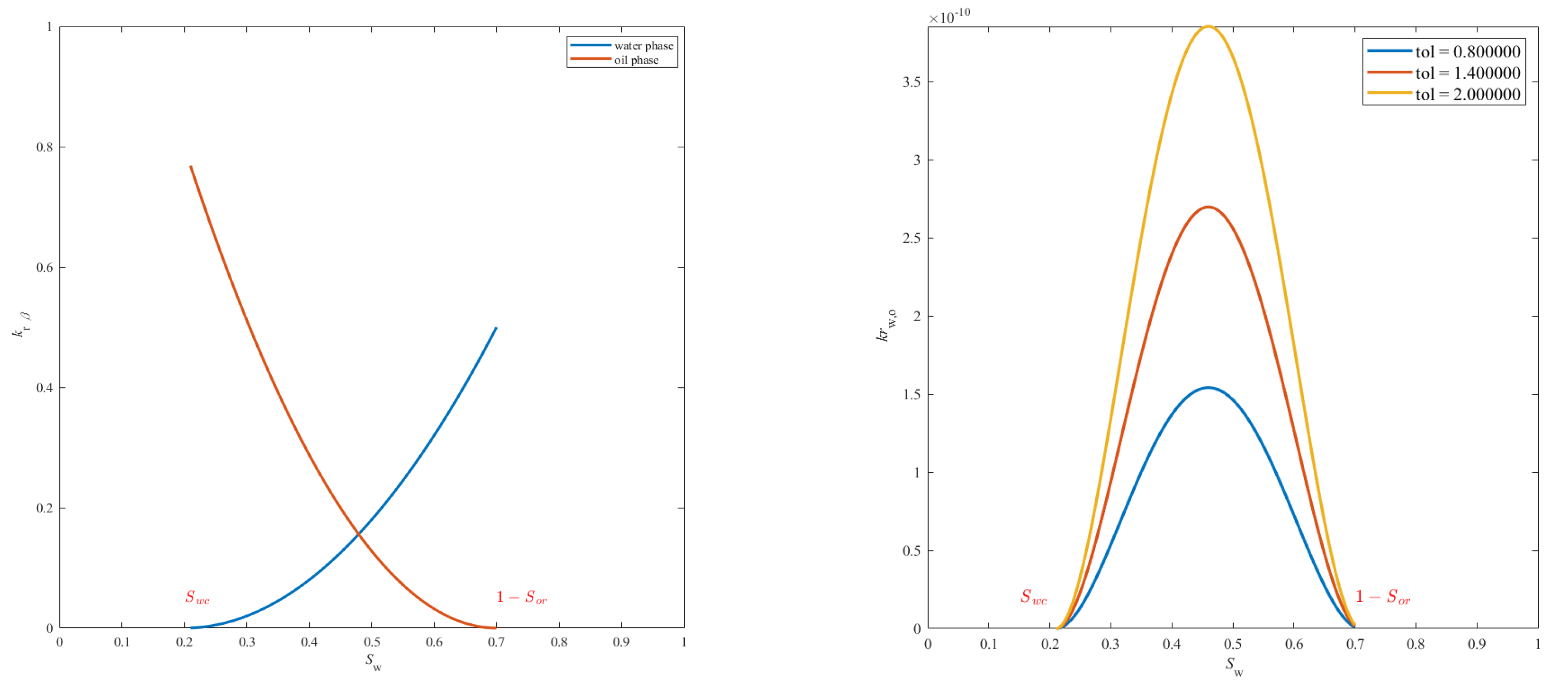
where $S_{wc}$ denotes the connate and $S_{or}$ is the residual oil saturation. $k_{rw}^{max}$ and $k_{ro}^{max}$ denote the maximal relative permeabilities for water and oil. $n_w$ and $n_o$ denote real numbers to fit observed laboratory data. The coupling terms in the system (3) are chosen as

$$k{r}_{o,w}={\left(S_w-S_{wc}\right)}^{n_{o,w}}{\left(1-S_w-S_{or}\right)}^{n_{w,o}},k{r}_{w,o}={\left(S_w-S_{wc}\right)}^{n_{o,w}}{\left(1-S_w-S_{or}\right)}^{n_{w,o}},$$

(16)

where $n_{o,w}$ and $n_{w,o}$ depend on laboratory observations. The capillary pressure is assumed to depend only on the water saturation as follows (Van Genuchten capillary pressure [28]):

$$p_{c,o,w}=\tau {(S{e}^{-1/m}-1)}^{1-m};with{S}_e=\frac{S_w-S_{wc}}{1-S_{wc}-S_{or}}$$

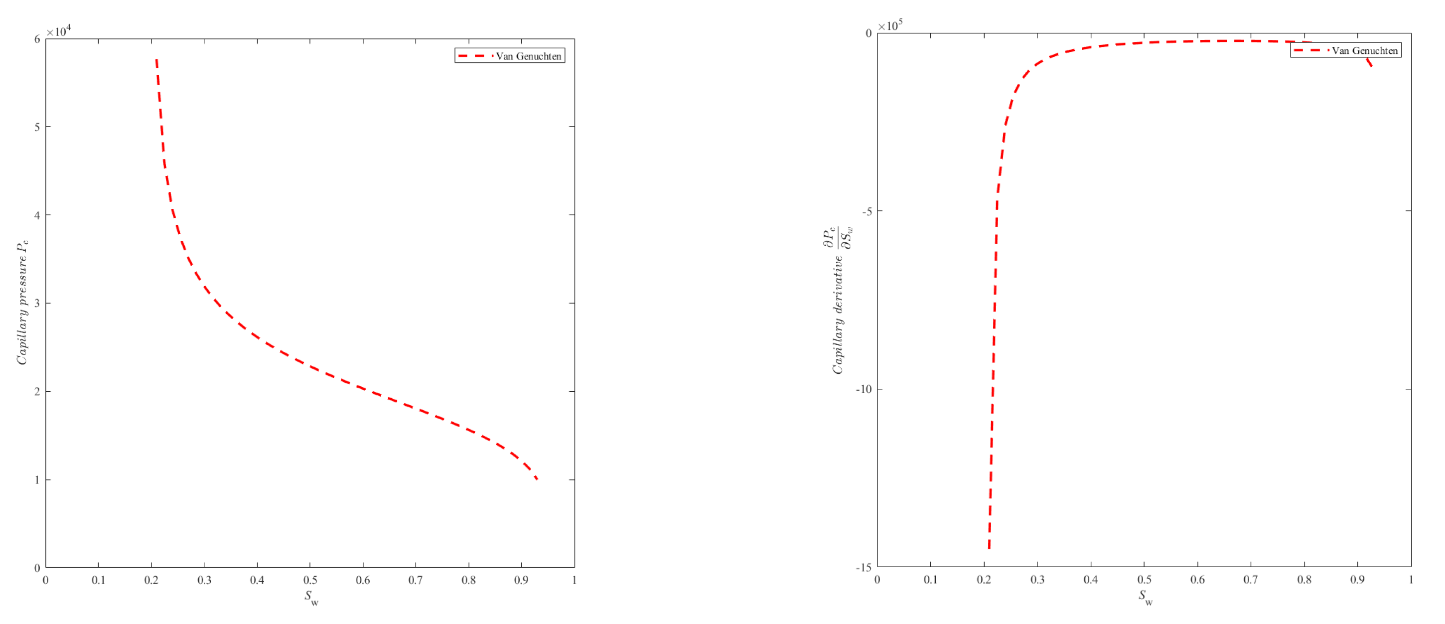
Observe that the capillary pressure (Figure 1) is a decreasing function of $S_w$, and therefore its derivative with respect to $S_w$ is negative and is given for all $S_{wc}\le S_w\le 1-S_{or}$ by

$$\frac{d{p}_{c,o,w}}{d{S}_w}=-\frac{1-m}{m}\tau \left(\frac{S_e^{-1-\frac{1}{m}}}{1-S_{wc}-S_{or}}{(S_e^{-1/m}-1)}^{-m}\right).$$

(17)

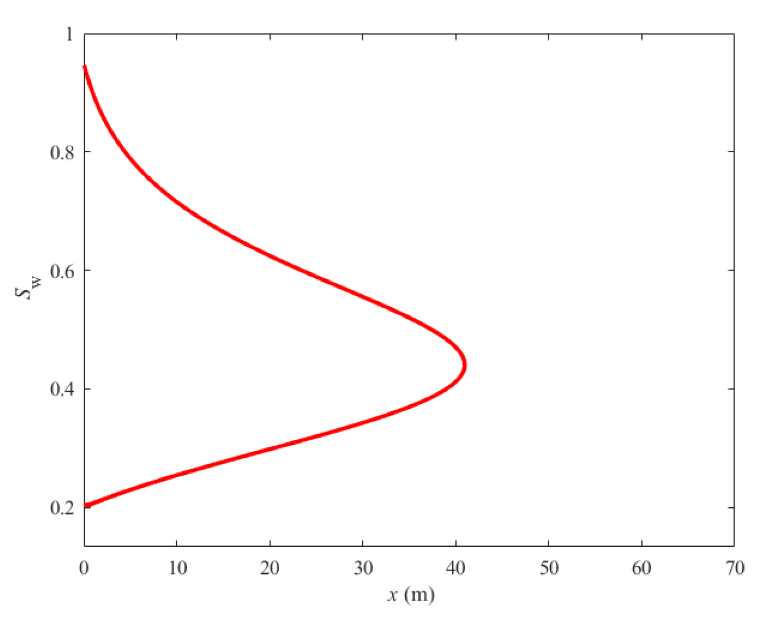
It is worth mentioning that the water fractional flow expression (9) involves the derivative with respect to space of the capillary pressure. Using the chain rule (13), one can infer that $\frac{\partial p_{c,o,w}}{\partial x}>0$ thanks to the typical profile of the water saturation in terms of x as shown in Figure 2.

Since the capillary pressure contributes to the water saturation dynamics, as per Equation (14), one can expect that its maximum influence is reached at a maximum of its derivative with respect to the water saturation, which corresponds to the zero of the expression (17), in particular at

$$S_w=S_{wc}+{\displaystyle \frac{1-S_{wc}-S_{or}}{{(1+m)}^m}}$$

Therefore, one approach could be to neglect the capillary pressure and consider it only close to the front where it is expected to have significant contribution. In addition, thanks to the sign of the gradient of the capillary pressure, one can expect that this enhances the front penetration velocity and introduces some diffusion to the system which in turn removes the sharp singularity at the front of the Buckley–Leverett solution. Our main interest in this paper is the comparison between the coupled system given by (3) and the classical Darcy’s approach described in (2), and therefore we both respective solutions presented below are obtained numerically using a Runge–Kutta approach.

To determine the front position, the equation to be solved reads

$${\left.\frac{dx}{dt}\right|}_{S_w}={\left.\frac{q_t}{A\varphi }\left\{\frac{k}{v_t}\frac{\partial S_w}{\partial x}\left\{{\displaystyle \frac{\partial f_w^1}{\partial S_w}}\frac{\partial p_{c,o,w}}{\partial S_w}+f_w^1{\displaystyle \frac{{\partial }^2{p}_{c,o,w}}{{\partial }^2{S}_w}}\right\}+{\displaystyle \frac{\partial f_w^2}{\partial S_w}}\right\}\right|}_t$$

(18)

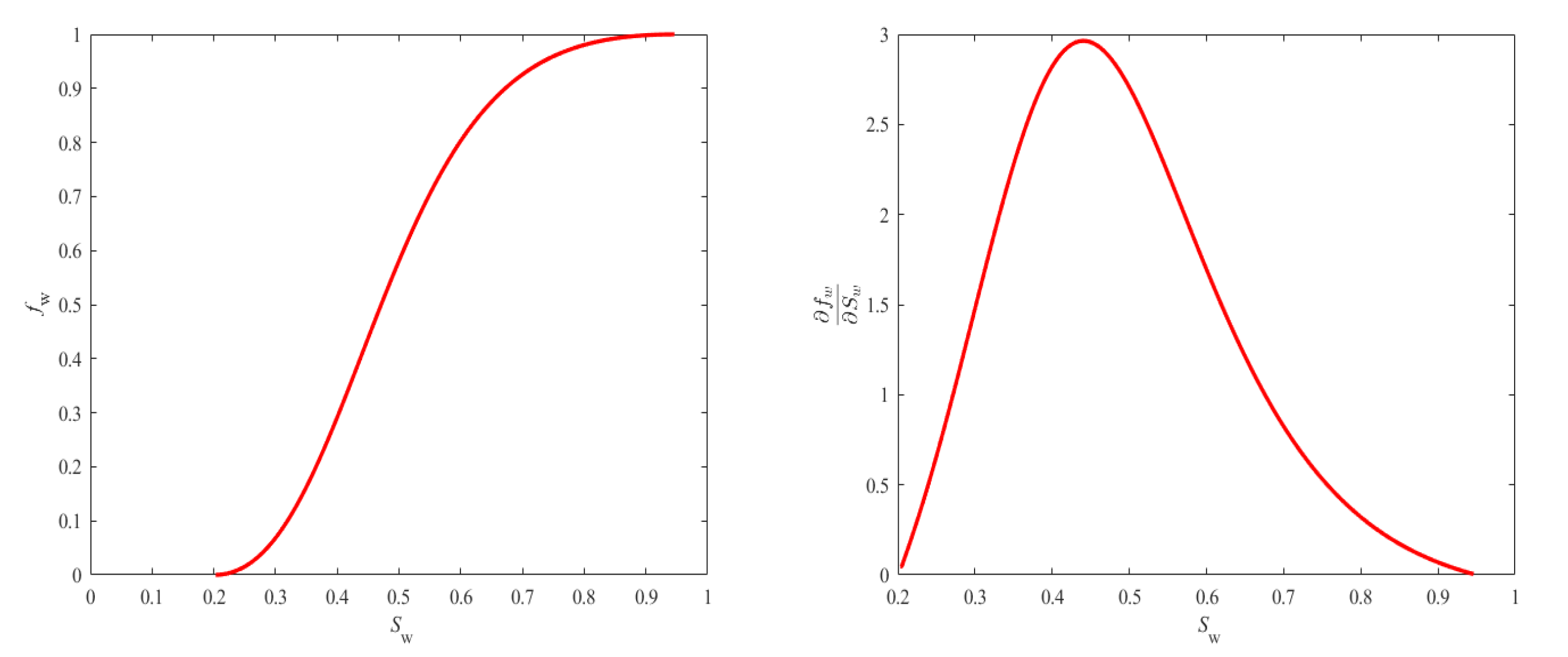
This equation can be solved using classical numerical methods by discretizing in time, space and water saturation. It is rather well-known that the difficulty resides in the fact that the typical water fractional flow curve has an inflection point, which provides two values of water saturation at the same time, since $\frac{d{f}_w}{d{S}_w}$ will reach a maximum value ((see Figure 3) for typical examples with capillary pressure).

One of the most commonly used methods to estimate the position of the schok water saturation front, solution of the Buckley–Leverett equation, is the simple and elegant Welge graphical method, [21]. The basic idea of the Welge’s method is based on the observation that, starting from the injection point, traveling velocities of a saturation will increase, with an increase in saturation initially from its connate value, until the curve of the derivative of the water fractional flow with respect to the water saturation attains a maximum value. Therefore, the points where the curve of the fractional flow indicates a decreasing velocity with increasing saturation, a significant change is needed that is a schok is formed. From the graphical point of view, this method, using Welge’s method to localize the front water saturation $S_{wf}$, amounts to determining the coordinates of to the point $(S_{wf},f_w\left(S_{wf}\right))$ such that the line passing through this point and the connate water saturation point $(S_{wc},0)$ is tangent to the fractional flow curve. Let us mention that we shall use the Welge’s method only for comparison purposes between different scenarios to see graphically that the front water saturation position changes when considering different values of the coupling cross-terms. However, for the the determination of the breakthrough time, we solve Buckley–Leverett numerically. Observe that, in the presence of capillary pressure, there is no schok since the capillary pressure brings in some diffusion that removes the sharp singularity at the front of Buckley–Leverett equation.

In the sequel, we consider a one-dimensional, flow direction simulation with an horizontal reservoir which has a uniform cross-area A. We provide two scenarios

• Comparison: classical Darcy’s system vs coupled system with $k{r}_{o,w}=k{r}_{w,o}$ (see (19))
• Effect of non-symmetric coupling: coupled system with $k{r}_{o,w}=ϵk{r}_{w,o}$ (we refer to $ϵ$ as tolerance). For more examples, see (see (20))

In what follows, we shall use two sets of data. The first is theoretical and aims at showing the difference between both models. The second set of data is dedicated to a physically realistic case. In particular, we shall consider the following data:

(a)

First set of data

Parameters	Value	Unit
Length of formation, L	1000.0	[m]
Cross-area of reservoir, A	${10}^4$	[m${}^2$]
Absolute permeability, k	2.96 $\times {10}^{-13}$	[m${}^2$]
Oil phase viscosity, ${\mu }_o$	5 $\times {10}^{-3}$	[Pa.s]
Water phase viscosity, ${\mu }_w$	${10}^{-3}$	[Pa.s]
Oil density, ${\rho }_o$	0.8 $\times {10}^3$	[kg/m${}^3$]
Water density, ${\rho }_w$	${10}^3$	[kg/m${}^3$]
Initial water injection rate, $q_t$	400	[m${}^3$/s]
Porosity, $\varphi$	0.30	[-]
Residual oil saturation, $S_{or}$	0.25	[-]
Connate water saturation, $S_{wc}$	0.20	[-]
Maximal relative permeability for oil, $k_{ro}^{max}$	0.8	[-]
Maximal relative permeability for water, $k_{rw}^{max}$	0.5	[-]
Power index of water relative permeability $n_w$	2.00	[-]
Power index of oil relative permeability, $n_o$	2.00	[-]
Power index of first coupling term $k{r}_{o,w}$, $n_{o,w}$	2.00	[-]
Power index of second coupling term $k{r}_{w,o}$, , $n_{w,o}$	2.00	[-]

(b)

Second set of data

Parameters	Value	Unit
Length of formation, L	3280	[ft]
Cross-area of reservoir, A	$10,764\times {10}^4$	[ft${}^2$]
Absolute permeability, k	300	[mD]
Oil phase viscosity, ${\mu }_o$	5	[cP]
Water phase viscosity, ${\mu }_w$	1	[cP]
Oil density, ${\rho }_o$	22.653	[kg/ft${}^3$]
Water density, ${\rho }_w$	28.316	[kg/ft${}^3$]
Initial water injection rate, $q_t$	2515.924	[bbl/s]
Porosity, $\varphi$	0.30	[-]
Residual oil saturation, $S_{or}$	0.25	[-]
Connate water saturation, $S_{wc}$	0.20	[-]
Maximal relative permeability for oil, $k_{ro}^{max}$	0.8	[-]
Maximal relative permeability for water, $k_{rw}^{max}$	0.5	[-]
Power index of water relative permeability $n_w$	2.00	[-]
Power index of oil relative permeability, $n_o$	2.00	[-]
Power index of first coupling term $k{r}_{o,w}$, $n_{o,w}$	2.00	[-]
Power index of second coupling term $k{r}_{w,o}$, , $n_{w,o}$	2.00	[-]

We shall consider the following two cases:

• The case of $k{r}_{o,w}=k{r}_{w,o}$, we choose

  $$\begin{array}{c}k{r}_{o,w}=k{r}_{w,o}={\left(S_w-S_{wc}\right)}^2{\left(1-S_w-S_{or}\right)}^2\hfill \end{array}$$

  (19)
• The case of $k{r}_{o,w}=\epsilon k{r}_{w,o}$ we choose:

  $$\begin{array}{c}k{r}_{o,w}={\left(S_w-S_{wc}\right)}^2{\left(1-S_w-S_{or}\right)}^2,k{r}_{w,o}={\displaystyle \frac{7}{5}}{\left(S_w-S_{wc}\right)}^2{\left(1-S_w-S_{or}\right)}^2\hfill \\ k{r}_{o,w}={\left(S_w-S_{wc}\right)}^2{\left(1-S_w-S_{or}\right)}^2,k{r}_{w,o}=2{\left(S_w-S_{wc}\right)}^2{\left(1-S_w-S_{or}\right)}^2\hfill \end{array}$$

  (20)

3.2. Numerical Results

In this section, we present few numerical simulations aiming at comparing the introduced coupled system (3) and the classical Darcy’s approach given by (2). The initial data, total constant velocity, and the system’s parameters are chosen as in the previous tables. The first example describes a comparison between the solution of the classical Darcy’s system (2) and the solution on the coupled Darcy’s system (3) by varying the tolerance $\epsilon$. For the first scenario of $k{r}_{w,o}=\epsilon k{r}_{o,w}$, we choose the following values for the tolerance $\epsilon$,

$$\epsilon =\left\{2,4,6\right\}.$$

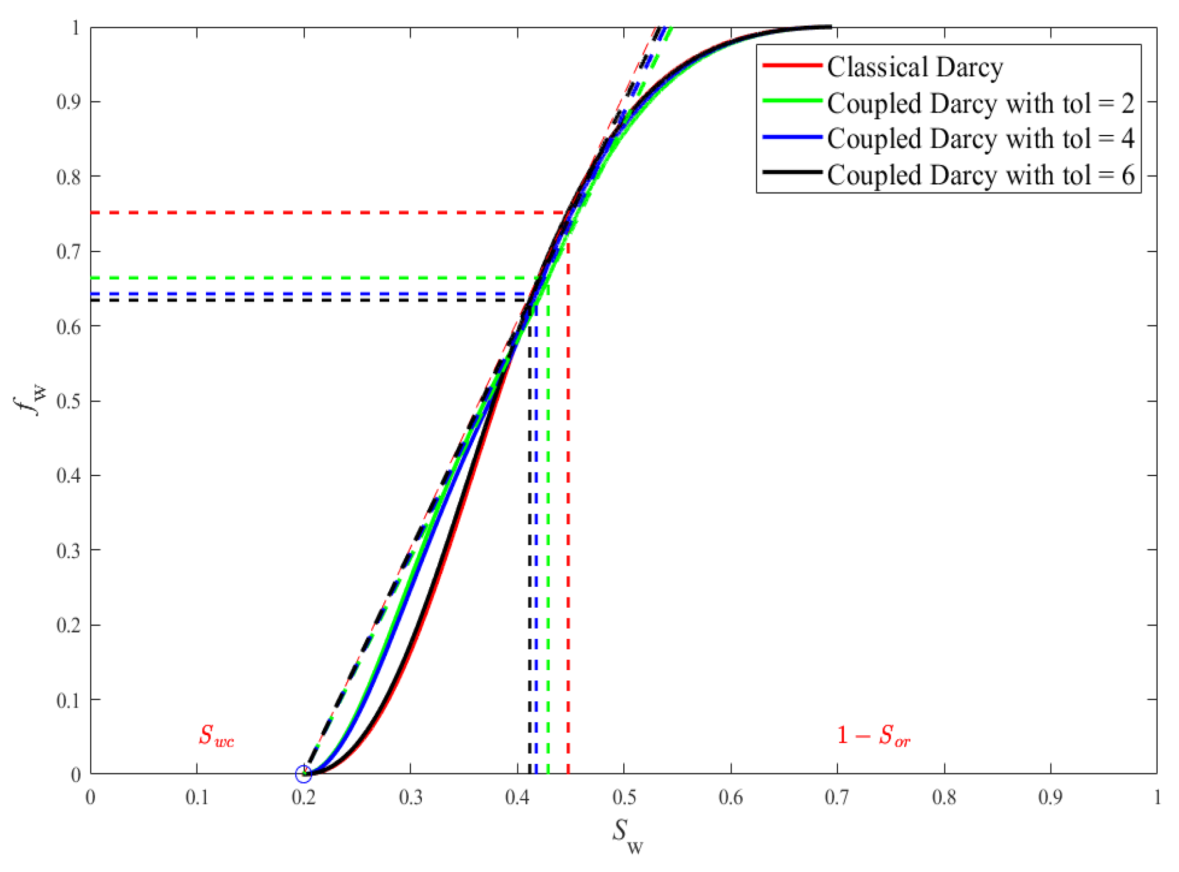
Figure 4 shows the classical graph of $k{r}_o,k{r}_w$, and ${\left(k{r}_{w,o}\right)}_i$, i = 1,...,3, corresponding to the tolerances above.

Figure 5 shows the fractional flow graph associated with the classical Darcy’s system together with the one associated with the coupled system for three values of tolerances as indicated above. For instance, if one chooses to use the Welge approach to locate the front, that is, if we trace a line passing through the saturation $S_{wc}$, corresponding to the beginning of the water injection, and tangent to the fractional flow, we observe different values of $S_{wf}$ clearly affecting the water front position and therefore its advance.

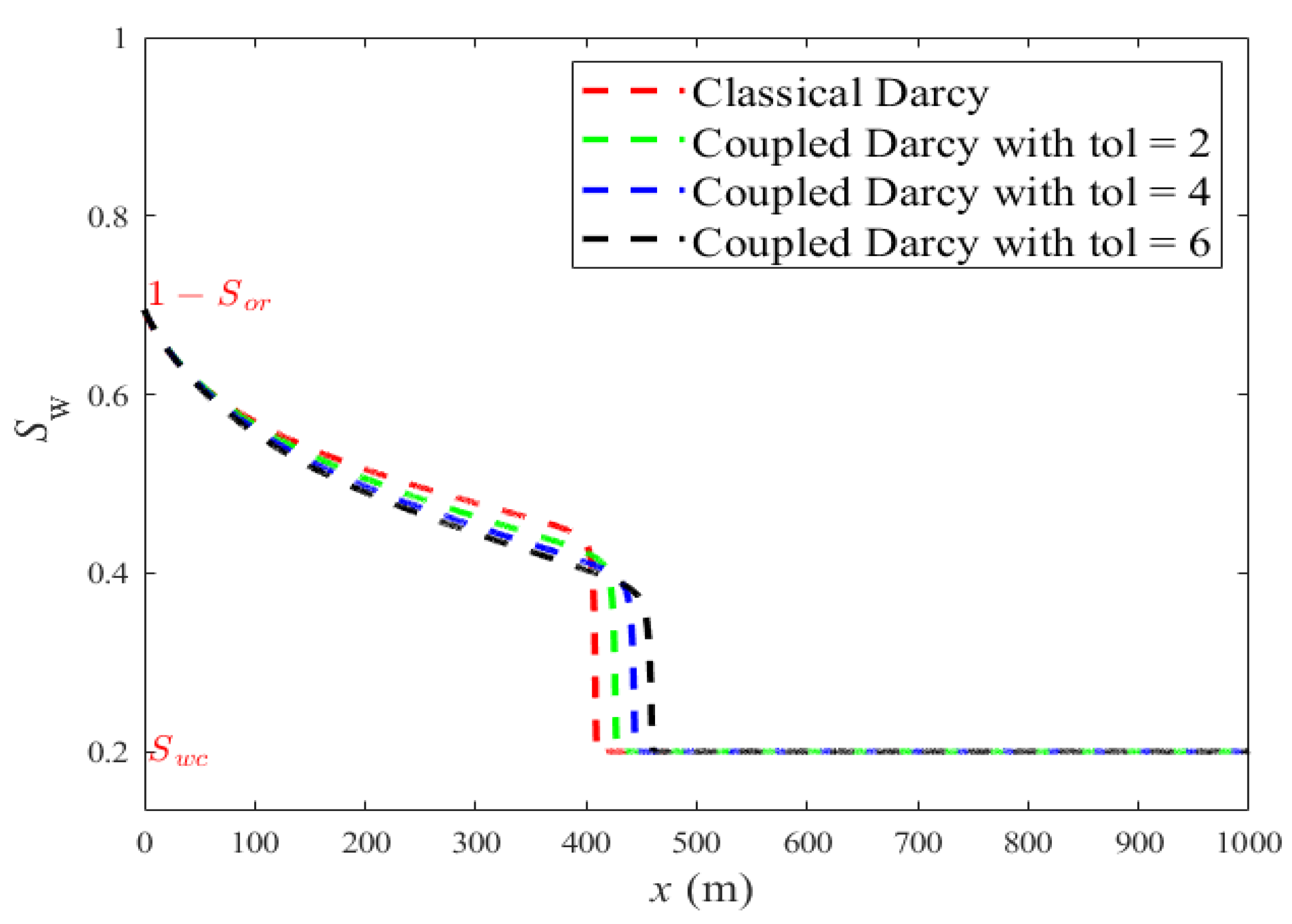
The associated water saturation profiles are shown in Figure 6. We observe a more advanced water saturation front position compared to the one corresponding to system (2) for all values of tolerances. The front position is in advance of approximatively 1.77%, 3.55%, and 5.14% after 1500 days, respectively to the chosen tolerances, compared to the classical Darcy’s one. Such differences clearly impact the volume of oil recovered from the reservoir.

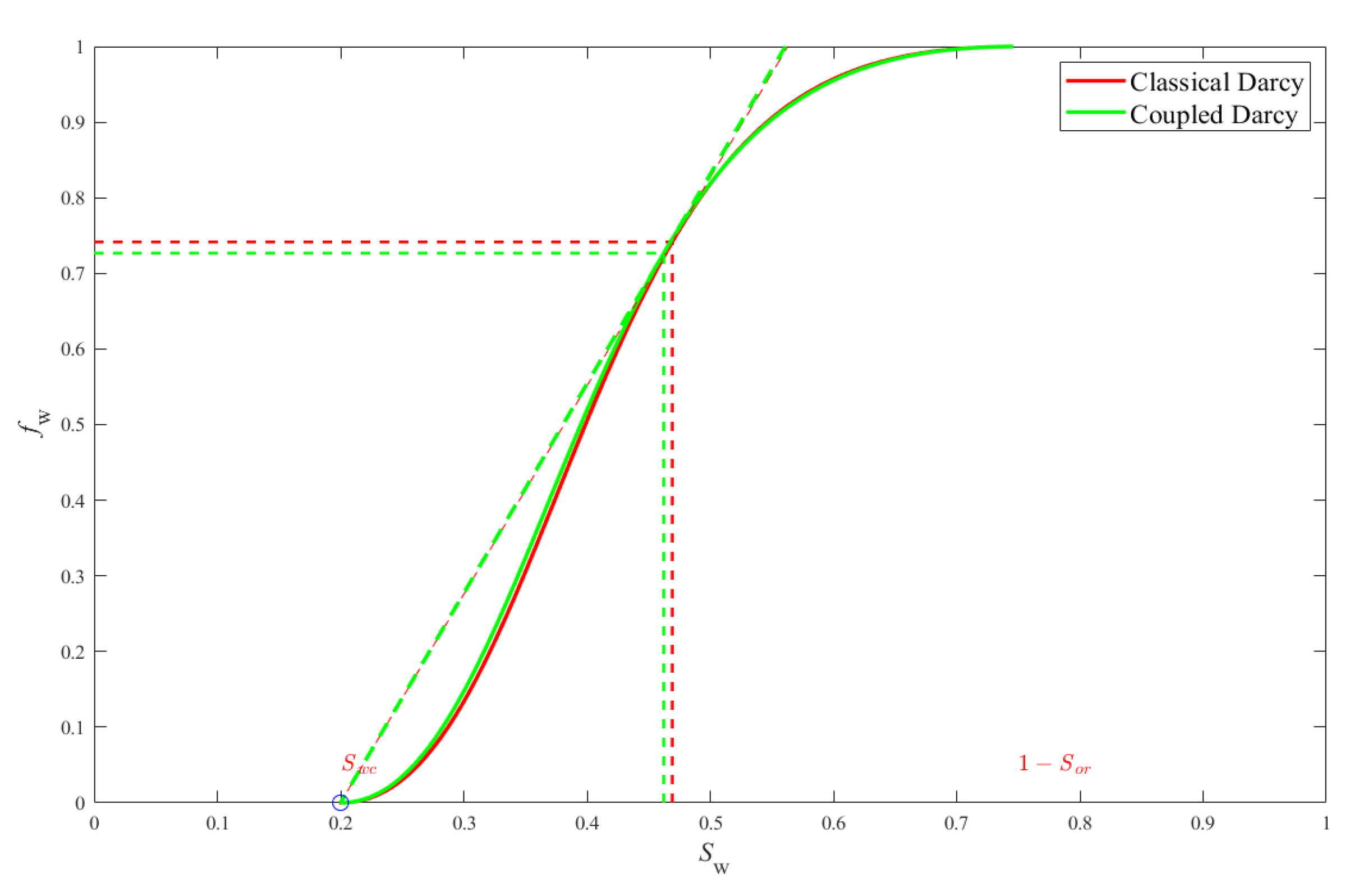
To emphasize the effect of coupling terms on the displacement of the two phase flow, a second scenario is considered. We assume that the permeabilities $k{r}_{o,w}$ and $k{r}_{w,o}$ are equal, and we consider the second set of data given in the table above. Figure 7 represents the graph of the water fractional flow for both systems (classical and coupled). The figure shows a difference in the water saturation front $S_{wf}$ obtained by Welge’s method, [21]. Therefore, one can see that, even in the case of $k{r}_{o,w}=k{r}_{w,o}$, a difference in the water saturation front position between both systems appears. Observe that, in this case, the cross-terms are not equal (see below for equal cross-terms). Such difference can be clearly seen in the graph of the respective water saturation profiles presented in Figure 8.

Eventually, let us consider the case of the specific tolerance $\epsilon$ given by

$$\epsilon ={\displaystyle \frac{{\mu }_w}{{\mu }_o}},$$

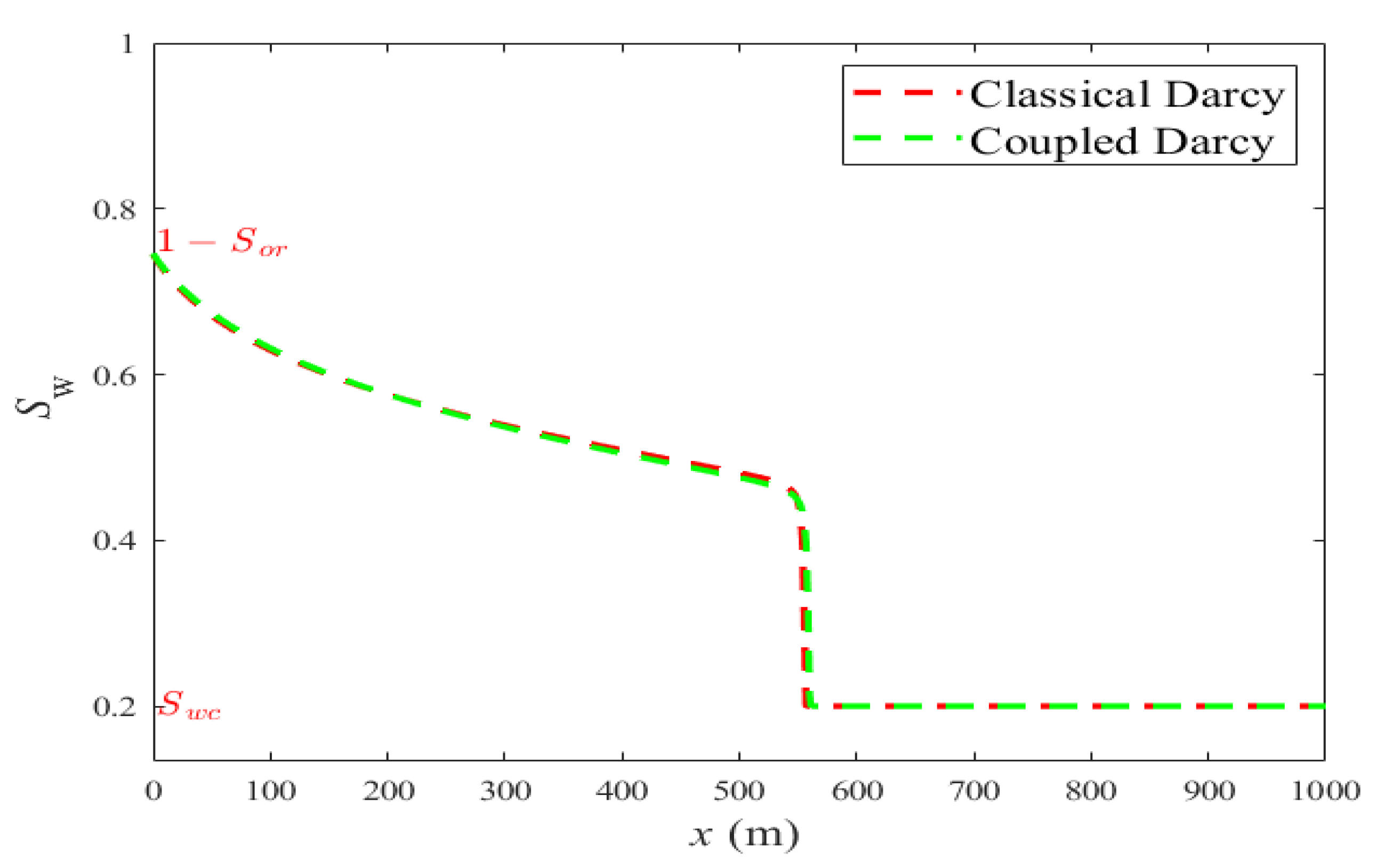
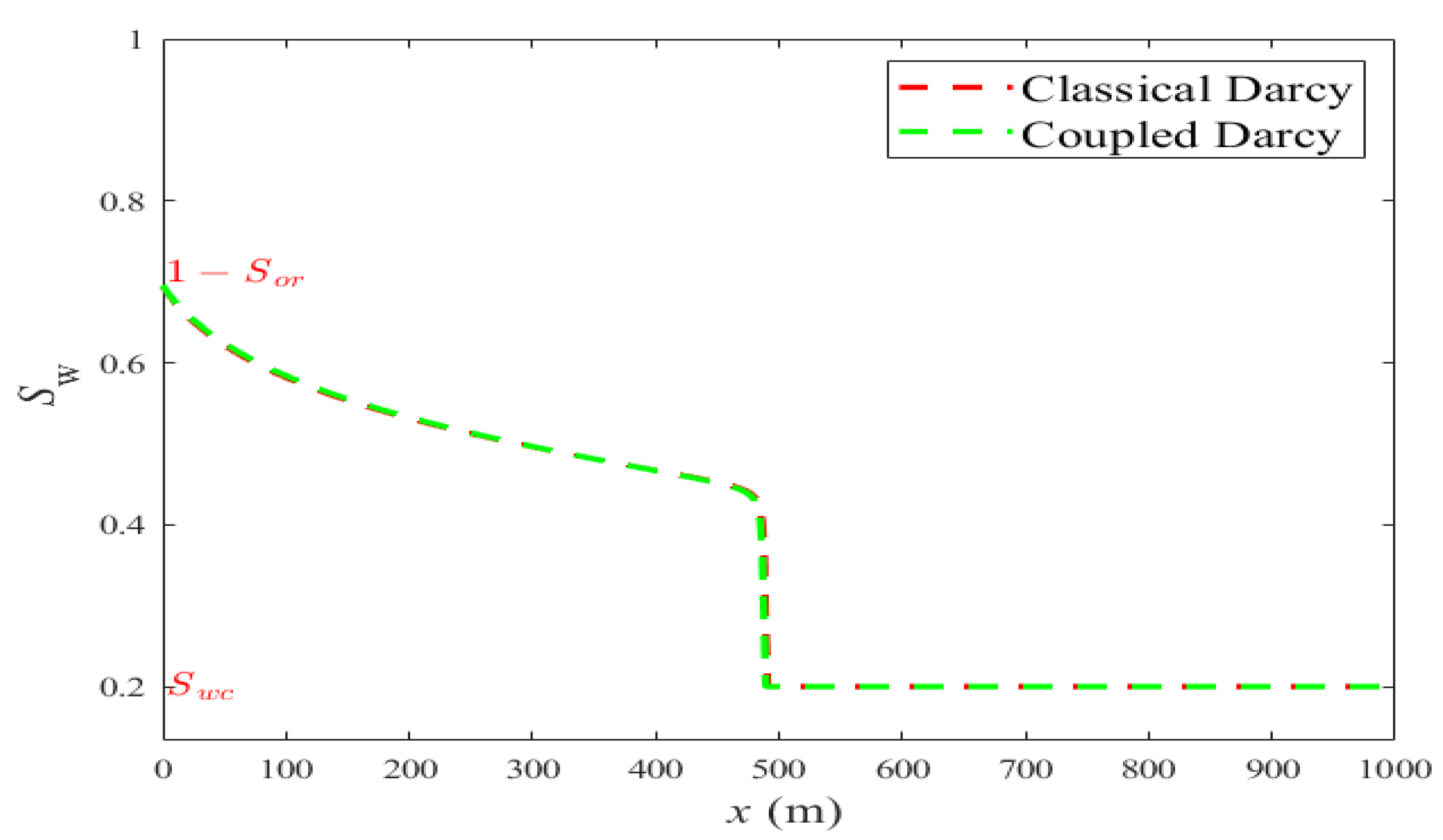
which implies that the cross-terms coefficients are equal (cross-mobilities). In this scenario, Figure 9 shows that there is no difference in the water saturation front position which is rather intuitive and expected.

All in all, for a given displacement system with constant water injection rate, the solution of the Equation (11), corresponding to the coupled system (3) that is the water saturation front, depends clearly on the amplitude of the cross-terms and not only on the pressure gradients. Indeed, Figure 6 and Figure 8 show a consequent difference, compared to the classical Darcy’s system (2) in terms of water front position compared to Figure 9.

As an application of the previous results, we compute the breakthrough time for both scenarios using the following formula:

$$t_L={\displaystyle \frac{A\varphi x_L}{q_t{\left.{\displaystyle \frac{\partial f_w}{\partial S_w}}\right|}_{S_{wf}}}}$$

(21)

For the first scenario:

Classical Darcy	Tolerance  $\mathbf{\epsilon }=\mathbf{0}.\mathbf{8}$	Tolerance  $\mathbf{\epsilon }=\mathbf{1}.\mathbf{4}$	Tolerance  $\mathbf{\epsilon }=\mathbf{2}$
$t_L=2.7219\times {10}^3$ days	$t_L=2.5843\times {10}^3$ days	$t_L=2.5397\times {10}^3$ days	$t_L=2.5024\times {10}^3$ days

For the second scenario:

Classical Darcy	Coupled Darcy with  ${\mathit{kr}}_{\mathbf{w},\mathbf{o}}=\mathit{kr}\mathbf{o},\mathbf{w}$
$t_L=2.7219\times {10}^3$ days	$t_L=2.7071\times {10}^3$ days

4. Discussion

4.1. On the Fractional Flow

As shown in the previous section, the cross-terms affect the water front position in the reservoir, and therefore play a role in the description of the flow dynamic when compared to the classical multiphase Darcy’s approach (2). In this section, we make few comments on the fractional water flow expression associated with the coupled system (3), and given by (9). It is rather clear that (9) can be reformulated as follows:

$$\begin{array}{ccc}\hfill f_w& =& \frac{\left[1-\frac{M_{o,w}}{M_o}\frac{M_{w,o}}{M_w}\right]\frac{k{M}_o}{v_t}{\partial }_x{p}_{c,o,w}+\left[1+\frac{M_{w,o}}{M_w}\right]}{\left(1+\frac{M_o}{M_w}\right)\left[1+\frac{M_{o,w}+M_{w,o}}{M_o+M_w}\right]}.\hfill \end{array}$$

(22)

The classical Darcy’s approach can be seen as a limiting, or particular case, of the coupled multiphase approach we developed in this paper. Indeed, setting $M_{o,w}=M_{w,o}=0$ reduces system (3) to the classical Darcy’s system (2) (with $\mathbf{g}=0$), and the fractional flow Formula (22) reduces to the well-known water fractional flow expression associated with system (2). More precisely, setting $M_{o,w}=M_{w,o}=0$ in (9), we get

$$\begin{array}{c}\hfill f_w^{\mathrm{Darcy}}=\frac{M_o{M}_w\frac{k{\partial }_x{p}_{c,o,w}}{v_t}+M_w}{M_o+M_w}=\frac{\frac{k{M}_o}{v_t}{\partial }_x{p}_{c,o,w}+1}{1+\frac{M_o}{M_w}}.\end{array}$$

(23)

This is a well-known formula when capillary pressure is considered in the classical Darcy’s approach (2). Clearly, when the capillary pressure is neglected, the formula reduces to

$$\begin{array}{c}\hfill f_w^{\mathrm{Darcy}}=\frac{1}{1+\frac{M_o}{M_w}}.\end{array}$$

(24)

Comparing the expressions (22) and (23), we see that the contribution of the coupling cross-terms in system (3) is described through the three terms between the square brackets. The expression (22) raises the natural question of the choices $M_{w,o}=M_{w,}$ and $M_{o,w}=M_o$ leading to

$$f_w=\frac{M_w}{M_o+M_w}=\frac{1}{1+\frac{M_o}{M_w}},$$

(25)

corresponding to the classical Darcy’s water fractional flow (24) when the capillary pressure is neglected or equal zero. This formula can be justified using a rescaling argument. Indeed, in the case of $M_{w,o}=M_{w,}$ and $M_{o,w}=M_o$, system (3) turns out to be

$$\begin{array}{c}{\displaystyle v_o=-k{M}_o{\partial }_x{p}_o-k{M}_o{\partial }_x{p}_w,}\hfill \\ {\displaystyle v_w=-k{M}_w{\partial }_x{p}_w-k{M}_w{\partial }_x{p}_o.}\hfill \end{array}$$

Using the capillary pressure definition, we can write

$$\begin{array}{c}{\displaystyle v_o=-2k{M}_o{\partial }_x{p}_o+k{M}_o{\partial }_x{p}_{c,o,w}=-k{M}_o{\partial }_x\left(2p_o-p_{c,o,w}\right),}\hfill \\ {\displaystyle v_w=-2k{M}_w{\partial }_x{p}_w-k{M}_w{\partial }_x{p}_{c,o,w}=-k{M}_w{\partial }_x\left(2p_w+p_{c,o,w}\right).}\hfill \end{array}$$

Denoting ${\tilde{p}}_o:=2p_o-p_{c,o,w}$, and ${\tilde{p}}_w:=2p_w+p_{c,o,w}$, this system turns out to be the classical Darcy’s system with oil and water phases velocities given by $v_o$ and $v_w$, respectively, but with oil and water phases pressures given by ${\tilde{p}}_o$ and ${\tilde{p}}_w$, respectively. Therefore, the associated water fractional flow is given by the classical formula:

$$\begin{array}{c}\hfill f_w^{\mathrm{Darcy}}=\frac{1+\frac{k{M}_o}{v_t}{\partial }_x{\tilde{p}}_{c,o,w}}{1+\frac{M_o}{M_w}}=\frac{1+\frac{k{M}_o}{v_t}{\partial }_x\underset{=0}{\underbrace{(2p_o-p_{c,o,w}-2p_w-p_{c,o,w})}}}{1+\frac{M_o}{M_w}},\end{array}$$

which justifies the Formula (25). In particular, this infers that one can perform post calculation based on the classical Darcy’s system (2) (with $\mathbf{g}=0$) to include the effect of each phase on the other in the case of cross-terms chosen such that $M_{w,o}=M_{w,}$ and $M_{o,w}=M_o$, which is in the case of

$$k{r}_{w,o}=k{r}_w\mathrm{and}k{r}_{o,w}=k{r}_o,$$

under the assumption that the capillary pressure depends only on the water saturation. Indeed, let $(v_o,p_o)$ and $(v_w,p_w)$ be as in system (2) (with $\mathbf{g}=0$), thus $(v_o,{\tilde{p}}_o=\frac{p_o+p_{c,o,w}}{2})$ and $(v_w,{\tilde{p}}_w=\frac{p_w+p_{c,o,w}}{2})$ satisfy the system

$$\begin{array}{c}{\displaystyle v_o=-k{M}_o{\partial }_x{\tilde{p}}_o-k{M}_o{\partial }_x{\tilde{p}}_w,}\hfill \\ {\displaystyle v_w=-k{M}_w{\partial }_x{\tilde{p}}_w-k{M}_w{\partial }_x{\tilde{p}}_o,}\hfill \end{array}$$

and we refer to Section 4.2 for a general algorithm scheme allowing to take into account any cross-terms that is independent of $M_o$ and $M_w$ (that is, $k{r}_o$ and $k{r}_w$).

A situation that might be physically relevant is to consider the $M_{w,o}=0$ and $M_{o,w}\ne 0$ leading to the following semi-coupled system:

$$\begin{array}{c}{\displaystyle v_o=-k{M}_o{\partial }_x{p}_o-k{M}_{o,w}{\partial }_x{p}_w,}\hfill \\ {\displaystyle v_w=-k{M}_w{\partial }_x{p}_w.}\hfill \end{array}$$

Thanks to (22), the associated water fractional flow expression reads

$$\begin{array}{ccc}\hfill f_w& =& \frac{1}{\left[1+\frac{M_{o,w}}{M_o+M_w}\right]}\frac{\frac{k{M}_o}{v_t}{\partial }_x{p}_{c,o,w}+1}{1+\frac{M_o}{M_w}}<\frac{\frac{k{M}_o}{v_t}{\partial }_x{p}_{c,o,w}+1}{1+\frac{M_o}{M_w}},\hfill \end{array}$$

for all water saturation $S_w$ since $1+\frac{M_{o,w}}{M_o+M_w}>1$. Since the right-hand side of the latter inequality corresponds to the water fractional flow associated with the classical Darcy’s approach, one can argue that the derivative of $f_w$ with respect to the saturation $S_w$ will reach a smaller maximum than any classical Darcy’s system fractional flow. In particular, this means that, if we consider the same value for $S_{wc}$ for both systems, and use Welge’s approach, then the slope of the tangent to $f_w$ passing through $S_{wc}$ is smaller than the slope of Darcy’s classical system, suggesting a larger value for $S_{wf}$ in the case of the semi-coupled system. This is coherent with the fact that, if $M_{o,w}<<M_o+M_w$ (in the sense of $M_{o,w}$ is very small compared to $M_o+M_w$), then the factor ${(1+M_{o,w}/(M_o+M_w))}^{-1}$ is very close to 1, and therefore the effect of the semi-coupling term is minimal compared to the classical Darcy’s system.

In addition, observe that Formula (22) suggests, at least formally, that, if $M_{o,w}<<M_o$ and $M_{w,o}<<M_w$ at any space position x in the reservoir and time t, then the graph of the water fractional flow of the coupled system (3) will be very close to the graph of the water fractional flow corresponding to the classical Darcy’s approach (2). Thus, one can reasonably expect that the slope of their respective tangents passing through $S_{wc}$ will be very close, and therefore so is the value of $S_{wf}$. This observation makes sense from the physical point of view, since such small coupling cross-terms are expected to have a very small effect and impact on the dynamic of the system, and can be seen as a very small perturbation of the classical Darcy’s system (2) (with $\mathbf{g}=0$).

4.2. Solution of Coupled System by a Decoupling Approach

Most of the industrial codes use the classical Darcy approach (2) to model multiphase flows, and any deviation from this scenario will be immediately termed “non Darcy flow”. In this section, we present a method allowing any classical existing code or software based on the classical Darcy’s approach to take into account the coupling between phases. The idea consists of solving the classical Darcy’s system (2) with modified permeabilities (or mobilities), and use the latter solution to obtain a second solution taking into account the effect of every phase on the other. Below, we present the idea in the case of two phases flow, for simplicity, but obviously it can be generalized to the case of more involved phases and higher dimensions. Following the notation of the previous section, we aim to solve system (1) where the oil and water velocities are described by the following modified Darcy’s system:

$$\begin{array}{c}{\displaystyle v_o=-k{\overline{M}}_o{\partial }_x{p}_o,}\hfill \\ {\displaystyle v_w=-k{\overline{M}}_w{\partial }_x{p}_w,}\hfill \end{array}$$

(26)

where we used the notation ${\overline{M}}_o=M_o+M_{w,o}$ and ${\overline{M}}_w=M_w+M_{o,w}$. This is nothing but Darcy’s classical system (2) (with $\mathbf{g}=0$) with modified permeabilities, that is, $M_o$ and $M_w$ are replaced by ${\overline{M}}_o$ and ${\overline{M}}_w$, respectively. Therefore, following the classical approach, a straightforward calculation shows that

$${\displaystyle {\partial }_x{p}_o=\frac{k{\overline{M}}_w{\partial }_x{p}_{c,o,w}-v_t}{k({\overline{M}}_o+{\overline{M}}_w)},\mathrm{and}{\partial }_x{p}_w=-\frac{k{\overline{M}}_o{\partial }_x{p}_{c,o,w}+v_t}{k({\overline{M}}_o+{\overline{M}}_w)},}$$

(27)

inferring the following water and oil velocities’ expressions

$$\begin{array}{cc}\hfill v_o& =\frac{-k{\overline{M}}_w{\partial }_x{p}_{c,o,w}+v_t}{1+\frac{{\overline{M}}_w}{{\overline{M}}_o}},\mathrm{and}{v}_w=\frac{k{\overline{M}}_o{\partial }_x{p}_{c,o,w}+v_t}{1+\frac{{\overline{M}}_o}{{\overline{M}}_w}}.\hfill \end{array}$$

Specifically, the water fractional flow expression reads

$$\begin{array}{c}\hfill f_w=\frac{\frac{k{\overline{M}}_o}{v_t}{\partial }_x{p}_{c,o,w}+1}{1+\frac{{\overline{M}}_o}{{\overline{M}}_w}}.\end{array}$$

(28)

Since all the mobilities and the capillary pressure are assumed to depend only on the water saturation, using this fractional expression the system (11) can be solved and a Buckley–Leverett solution obtained using, for instance, Welge’s approach or any numerical scheme.

In the sequel, using a velocity rescaling argument, we show that the fractional flow (28) determines uniquely the fractional flow associated with the coupled system (3). Hence, in order to solve (3), any existing code or software can be used to determine the fractional flow (and its graph) associated with the modified Darcy’s system (26), and therefore obtain the fractional flow (and its graph) associated (3), and eventually apply, Welge’s method, for instance, can be used to determine the water front. Indeed, we have the following

Lemma 1.

If $(v_o,p_o)$ and $(v_w,p_w)$ satisfy system (26), then $({\tilde{v}}_o,p_o)$ and $({\tilde{v}}_w,p_w)$ given by

$$\left\{\begin{array}{c}{\displaystyle {\tilde{v}}_o=v_o+\frac{k\left(M_{o,w}{\overline{M}}_o+M_{w,o}{\overline{M}}_w\right){\partial }_x{p}_{c,o,w}+(M_{o,w}-M_{w,o})v_t}{{\overline{M}}_o+{\overline{M}}_w},}\hfill \\ \\ {\displaystyle {\tilde{v}}_w=v_w-\frac{k\left(M_{o,w}{\overline{M}}_o+M_{w,o}{\overline{M}}_w\right){\partial }_x{p}_{c,o,w}+(M_{o,w}-M_{w,o})v_t}{{\overline{M}}_o+{\overline{M}}_w},}\hfill \end{array}\right.$$

(29)

satisfy the following system

$$\begin{array}{c}{\displaystyle {\tilde{v}}_o=-k{M}_o{\partial }_x{p}_o-k{M}_{o,w}{\partial }_x{p}_w,}\hfill \\ {\displaystyle {\tilde{v}}_w=-k{M}_w{\partial }_x{p}_w-k{M}_{w,o}{\partial }_x{p}_o.}\hfill \end{array}$$

(30)

Proof. 

First, observe that ${\tilde{v}}_o+{\tilde{v}}_w=v_o+v_w=v_t$ which is constant as per the incompressibility property preserved by the flow. On the one side, thanks to (27), we can write

$$\frac{k{\overline{M}}_w{\partial }_x{p}_{c,o,w}}{{\overline{M}}_o+{\overline{M}}_w}=k{\partial }_x{p}_o+\frac{v_t}{{\overline{M}}_o+{\overline{M}}_w},\mathrm{and}\frac{k{\overline{M}}_o{\partial }_x{p}_{c,o,w}}{{\overline{M}}_o+{\overline{M}}_w}=-k{\partial }_x{p}_w-\frac{v_t}{{\overline{M}}_o+{\overline{M}}_w}.$$

On the opposite side, following (29)${}_1$, we have

$$\begin{array}{cc}\hfill {\tilde{v}}_o& =v_o+M_{o,w}\frac{k{\overline{M}}_o{\partial }_x{p}_{c,o,w}}{{\overline{M}}_o+{\overline{M}}_w}+M_{w,o}\frac{k{\overline{M}}_w{\partial }_x{p}_{c,o,w}}{{\overline{M}}_o+{\overline{M}}_w}+\frac{M_{o,w}-M_{w,o}}{{\overline{M}}_o+{\overline{M}}_w}{v}_t\hfill \\ \hfill & =-k{\overline{M}}_o{\partial }_x{p}_o+M_{o,w}\left(-k{\partial }_x{p}_w-\frac{v_t}{{\overline{M}}_o+{\overline{M}}_w}\right)+M_{w,o}\left(k{\partial }_x{p}_o+\frac{v_t}{{\overline{M}}_o+{\overline{M}}_w}\right)+\frac{M_{o,w}-M_{w,o}}{{\overline{M}}_o+{\overline{M}}_w}{v}_t\hfill \\ \hfill & =-k{\overline{M}}_o{\partial }_x{p}_o-k{M}_{o,w}{\partial }_x{p}_w+k{M}_{w,o}{\partial }_x{p}_o\hfill \\ \hfill & =-k(M_o+M_{w,o}){\partial }_x{p}_o-k{M}_{o,w}{\partial }_x{p}_w+k{M}_{w,o}{\partial }_x{p}_o\hfill \\ \hfill & =-k{M}_o{\partial }_x{p}_o-k{M}_{o,w}{\partial }_x{p}_w,\hfill \end{array}$$

which is the desired result. The calculation for ${\tilde{v}}_o$ uses the change of variable given by (29)${}_1$ and the same argument we used above, then we omit it. □

In particular, the previous lemma allows us to write a relation between fractional flows of both system. In fact, using the Formula (28), we have

$$\begin{array}{cc}\hfill {\tilde{f}}_w& =f_w-\frac{\left(M_{o,w}{\overline{M}}_o+M_{w,o}{\overline{M}}_w\right)}{{\overline{M}}_o+{\overline{M}}_w}\frac{k{\partial }_x{p}_{c,o,w}}{v_t}-\frac{M_{o,w}-M_{w,o}}{{\overline{M}}_o+{\overline{M}}_w}\hfill \\ \hfill & =f_w-\frac{\left(M_{o,w}{\overline{M}}_o+M_{w,o}{\overline{M}}_w\right)}{{\overline{M}}_o+{\overline{M}}_w}\left(\frac{{\overline{M}}_o+{\overline{M}}_w}{{\overline{M}}_o{\overline{M}}_w}{f}_w-\frac{1}{{\overline{M}}_o}\right)-\frac{M_{o,w}-M_{w,o}}{{\overline{M}}_o+{\overline{M}}_w}\hfill \\ \hfill & =\frac{M_o{M}_w-M_{o,w}{M}_{wo}}{(M_o+M_{w,o})(M_w+M_{o,w})}{f}_w+\frac{M_{w,o}}{M_o+M_{w,o}}.\hfill \end{array}$$

(31)

Now, any existing code or software can easily solve system (1) with the oil and water velocities given by system (26), by only modifying the permeabilities input, which are assumed to depend analytically on the water saturation. Next, the value of the fractional flow of the coupled system (3) can be post calculated using the Formula (31). Eventually, any standard method, for instance analytical or Welge’s method, can be used to find the water front corresponding to the coupled system (3).

Observe that, setting formally the cross-terms $M_{o,w}=M_{w,o}$ in (31), we obtain ${\tilde{f}}_w=f_w$ given by (28) (corresponding to (23) by setting $M_{w,o}=0$ in (28) since system (26) turns out to be the classical Darcy’s system now). Furthermore, observe that, if the cross-terms are chosen such that $M_o=M_{o,w}$ and $M_w=M_{w,o}$, then we get

$${\tilde{f}}_w=\frac{1}{1+\frac{M_o}{M_w}},$$

which is the same formula as (24) corresponding to the classical Darcy’s system (2) (with $\mathbf{g}=0$). Eventually, let us point out that one cannot expect a physical interpretation from the expression (31) since the system (26) is not physical, but rather an artificial mathematical system that can be solved using standard petroleum solutions and its artificial solution manipulated to obtain a solution of the physical system (3).

5. Conclusions

In this paper, a mathematical model describing the behavior of a multiphase flow system taking into account the effect of one phase on the other, through a mathematical coupling between the phases, was considered. The coupling is modeled through cross-terms involving the pressure gradients multiplied by respective pseudo-mobilities. In comparison to the classical Darcy’s approach, we showed that a significant impact of such a coupling can occur in particular scenarios. This was shown by solving the associated Buckley–Leverett equations using a basic Runge–Kutta technique. In particular, the water front position is clearly shown to be significantly different from one model to the other. Obviously, several other aspects need to be investigated such as the injection rate, the effect of gravity, etc. Eventually, we investigated the mathematical relation between the coupled model and the decoupled one—namely, a classical Darcy’s type approach. Indeed, we were able to identify and introduce an artificial classical Darcy’s type model, with modified permeabilities (and therefore non-physical permeabilities), that has the advantage to be solvable by any existing software designed to solve the Classical Darcy’s system. Once the latter system was solved, and the velocities and the pressure obtained, we provided an explicit expression allowing a direct calculation of the solution of coupled system. More precisely, we proposed a method allowing to take into account the coupling between phases using any classical software able to solve classical Darcy’s system.

References

- Muskat, M. The Flow of Homogeneous Fluids through Porous Media; The Mapple Press Company: York, PA, USA, 1946. [Google Scholar]
- Kalaydjian, F. A macroscopic description of multiphase flow in porous media involving spacetime evolution of fluid/fluid interface. Transp. Porous Media 1987, 2, 537. [Google Scholar] [CrossRef]
- Kalaydjian, F. Origin and quantification of coupling between relative permeabilities for two-phase flows in porous media. Transp. Porous Media 1990, 5, 215. [Google Scholar] [CrossRef]
- Danis, M.; Quintard, M. Modélisation d’un écoulement diphasique dans une succession de pores. Rev. Inst. Français Pétrole 1984, 39, 37. [Google Scholar] [CrossRef]
- Rothman, D.H. Macroscopic laws for immiscible two-phase flow in porous media: Results from numerical experiments. J. Geophys. Res. Solid Earth 1990, 95, 8663. [Google Scholar] [CrossRef]
- Rose, W. Measuring transport coefficients necessary for the description of coupled two-phase flow of immiscible fluids in porous media. Transp. Porous Media 1988, 3, 163–171. [Google Scholar] [CrossRef]
- Rose, W. Petroleum reservoir engineering at the crossroads (Ways of thinking). Iran Petrol. Inst. Bull. 1972, 46, 23–27. [Google Scholar]
- Rose, W. Second thoughts on Darcy’s law. Iran Pet. Inst. Bull. 1974, 48, 25–30. [Google Scholar]
- De Gennes, P.G. Theory of slow biphasic flows in porous media. Phys. Chem. Hydrol. 1983, 4, 175–185. [Google Scholar]
- De la Cruz, V.; Spanos, T.J.T. Mobilization of oil ganglia. AIChE J. 1983, 29, 854–858. [Google Scholar] [CrossRef]
- Auriault, J.L.; Sanchez-Palencia, E. Remarques sur la loi de Darcy pour les écoulements biphasiques en milieu poreux. Z Theor. Appl. Mech. 1986, 141–156. [Google Scholar]
- Whitaker, S. Flow in porous media II: The governing equations for immiscible, two-phase flow. Transp. Porous Media 1986, 1, 105–125. [Google Scholar] [CrossRef]
- Spanos, T.J.T.; de la Cruz, V.; Hube, J.; Sharma, R.C. An analysis of Buckley–Leverett theory. J. Can. Petrol. Technol. 1986, 25, 71–75. [Google Scholar] [CrossRef]
- Kalaydjian, E.; Legait, B. Ecoulement lent à contre-courant de deux fluides non miscibles dans un capillaire présentant un rétrécissement. C.R. Acad. Sci. Paris. Ser. H 1987, 304, 869–872. [Google Scholar]
- Spanos, T.J.T.; de la Cruz, V.; Hube, J. An analysis of the theoretical foundations of relative permeability curves. AOSTRA J. Res. 1988, 4, 181. [Google Scholar]
- Kalaydjian, F.; Legait, B. Effets de la géométrie des pores et de la mouillabilité sur le déplacement diphasique à contre-courant en capillaire et en milieu poreux. Rev. Phys. Appl. 1988, 23, 1071–1081. [Google Scholar] [CrossRef]
- Rose, W. Attaching new meanings to the Equations of Buckley and Leverett. J. Pet. Sci. Eng. 1988, 1, 223–228. [Google Scholar] [CrossRef]
- Dullien, F.; Dong, M. Experimental determination of the flow transport coefficients in the coupled equations of two-phase flow in porous media. Transp. Porous Media 1996, 25, 97–120. [Google Scholar] [CrossRef]
- Pasquier, S.; Quintard, M.; Davit, Y. Modeling two-phase flow of immiscible fluids in porous media: Buckley–Leverett theory with explicit coupling terms. Phys. Rev. Fluids 2017, 2, 104101. [Google Scholar] [CrossRef] [Green Version]
- Buckley, S.E.; Leverett, M.C. Mechanism of fluid displacement in sands. Trans. AIME 1942, 146, 107–116. [Google Scholar] [CrossRef]
- Welge, H.J. A simplified method for computing oil recovery by gas or water drive. J. Pet. Technol. 1952, 4, 91–98. [Google Scholar] [CrossRef]
- Sheldon, J.W.; Cardwell, W.T., Jr. One-dimensional incompressible noncapillary two-phase fluid flow in a porous medium. Pet. Trans. AIME 1959, 216, 290–296. [Google Scholar] [CrossRef]
- McWhorter, D.B.; Sunada, D.K. Exact integral solutions for two-phase flow. Water Resour. Res. 1990, 26, 399–413. [Google Scholar] [CrossRef]
- Guérillot, D.; Kalaydjian, F. Application du Formalisme par Pression Globale a L’etude du Couplage Entre lois de Darcy Pour les Ecoulements Diphasiques en Milieu Poreux (Application of the Global Pressure Concept to the Study of Coupling between Generalized Darcy’s Laws for Two-Phase Flow in Porous Media Comptes Rendus); Serie II; Academie des Sciences: Paris, France, 1988; Volume 306, pp. 853–858. [Google Scholar]
- Chavent, G.; Cohen, G.; Jaffre, J.; Eyard, R.; Guerillot, D.R.; Weill, L. Discontinuous and Mixed Finite Elements for Two-Phase Incompressible Flow. SPE Reserv. Eng. 1990, 5, 567–575. [Google Scholar] [CrossRef]
- Willhite, G.P. Waterflooding; Society of Petroleum Engineers: Richardson, TX, USA, 1986. [Google Scholar]
- Brooks, R.H.; Corey, A.T. Hydraulic Properties of Porous Media. In Hydrology Papers; Colorado State University: Fort Collins, CO, USA, 1964; p. 3. [Google Scholar]
- Van Genuchten, M.T. A closed-form equation for predicting the hydraulic conductivity of unsaturated soils. Soil Sci. Soc. Am. J. 1980, 44, 892–898. [Google Scholar] [CrossRef] [Green Version]
Figure 1.
Van Genuchten capillary pressure and its derivative with respect to water saturation versus water saturation.
Figure 2.
Typical water saturation profile versus space position x.
Figure 3.
Typical fractional flow curve with respect to water saturation (left), and its derivative with respect to water saturation (right) versus water saturation.
Figure 4.
(Left) Relative permeability and in terms of water saturation. (Right) Coupling term permeability versus water saturation.
Figure 5.
Fractional flow in terms of water saturation (Time = 1500 days).
Figure 6.
Water Saturation profile in terms of the distance from the inlet (Time = 1500 days).
Figure 7.
Fractional flow curve in terms of water saturation (Time = 1500 days).
Figure 8.
Water Saturation profile in terms of distance from inlet (Time = 1500 days).
Figure 9.
Publisher’s Note: MDPI stays neutral with regard to jurisdictional claims in published maps and institutional affiliations. |
© 2020 by the authors. Licensee MDPI, Basel, Switzerland. This article is an open access article distributed under the terms and conditions of the Creative Commons Attribution (CC BY) license (http://creativecommons.org/licenses/by/4.0/).
Share and Cite
MDPI and ACS Style
Guérillot, D.; Kadiri, M.; Trabelsi, S. Buckley–Leverett Theory for Two-Phase Immiscible Fluids Flow Model with Explicit Phase-Coupling Terms. Water 2020, 12, 3041. https://doi.org/10.3390/w12113041
AMA Style
Guérillot D, Kadiri M, Trabelsi S. Buckley–Leverett Theory for Two-Phase Immiscible Fluids Flow Model with Explicit Phase-Coupling Terms. Water. 2020; 12(11):3041. https://doi.org/10.3390/w12113041
Chicago/Turabian StyleGuérillot, Dominique, Mostafa Kadiri, and Saber Trabelsi. 2020. "Buckley–Leverett Theory for Two-Phase Immiscible Fluids Flow Model with Explicit Phase-Coupling Terms" Water 12, no. 11: 3041. https://doi.org/10.3390/w12113041
Note that from the first issue of 2016, this journal uses article numbers instead of page numbers. See further details here.