Prediction of Streamflow Based on Dynamic Sliding Window LSTM

Abstract

The streamflow of the upper reaches of the Yangtze River exhibits different timing and periodicity characteristics in different quarters and months of the year, which makes it difficult to predict. Existing sliding window-based methods usually use a fixed-size window, for which the window size selection is random, resulting in large errors. This paper proposes a dynamic sliding window method that reflects the different timing and periodicity characteristics of the streamflow in different months of the year. Multiple datasets of different months are generated using a dynamic window at first, then the long-short term memory (LSTM) is used to select the optimal window, and finally, the dataset of the optimal window size is used for verification. The proposed method was tested using the hydrological data of Zhutuo Hydrological Station (China). A comparison between the flow prediction data and the measured data shows that the prediction method based on a dynamic sliding window LSTM is more accurate by 8.63% and 3.85% than the prediction method based on fixed window LSTM and the dynamic sliding window back-propagation neural network, respectively. This method can be generally used for the time series data prediction with different periodic characteristics.

1. Introduction

As the main basis for the comprehensive development and effective use of water resources, streamflow data is needed for the implementation of scientific management and optimal scheduling of water resources [1,2]. Streamflow prediction is an important part of hydrological calculations, and is also a prerequisite for flood prevention, disaster reduction, and the efficient use of water resources for sustainable development [3]. Therefore, it is of theoretical significance and practical value to study medium- and long-term streamflow predictions and to improve prediction accuracy [4,5].

Streamflow prediction can be divided into short- (hours or days), and mid- to long-term (months or years) flow prediction. It can also be divided into prediction methods based on causes and mathematical statistics. Currently, flow prediction methods are still not mature enough for wide application. This is because the streamflow is affected not only by natural factors (such as the ocean, atmosphere, geological environment, etc.), but also by human activities, which explains the great uncertainty in annual runoff. Some researchers have attempted to establish streamflow prediction models in which different weights are assigned to the factors affecting the annual runoff of rivers. For example, the ABCD model uses precipitation and potential evapotranspiration as inputs to simulate changes in evapotranspiration, runoff, water in the soil, and groundwater, based on which the monthly and yearly flow predictions can be made [6]. These methods rely on a variety of data collection methods and a large amount of collected data, and they can yield good prediction results for specific river channels. However, the application of these methods is limited for two reasons: The cost of data collection and analysis is high, and the models established for specific river channels are not very versatile. Moreover, many rivers lack long-term historical data, such as soil and precipitation data. The streamflow prediction methods based on mathematical statistics constitute the most widely used type of flow prediction method at present. This category includes traditional statistical methods, gray prediction [7], fuzzy prediction [8], neural network prediction [9,10,11,12,13], wavelet analysis [14,15,16], Markov chain [17], matrix factorization [18] and signal decomposition [19]. The data dimension (i.e., window) used by these methods is random and fixed, and the errors are large [20].

Previously proposed methods and models for the prediction of streamflow include a combination of phase space reconstruction (PSR) and artificial neural networks (ANNs) [21], a multilevel model combining Support Vector Machine (SVM) and the Fire-Fly Algorithm (FFA) while its output is fed to ANN [22], the hybrid model of a rolling mechanism and grey models (RMGM) with back propagation (RMGM-BP) and Elman Recurrent Neural Network (RMGM-ERNN) [23], a hybridization of random forest (RF) models with self-exciting threshold autoregressive (SETAR) model [24] and a combined modified empirical mode decomposition (EMD)-SVM (M-EMDSVM) model [25]. These methods can improve the prediction accuracy by using different models; however, such methods are not designed for time series data, and do not consider the characteristics of streamflow. In addition, some time series methods which have been to for streamflow prediction includes Long-Short Term Memory (LSTM) [26,27] and Gated Recurrent Unit (GRU) [28], a combined model of feed-forward neural network (FNN) with particle swarm optimization (PSO) and gravitational search algorithm (GSA) [29]. Here, LSTM is a special kind of RNN developed to avoid the long-term dependency problem, which makes it hard to learn dependencies over long time windows [30]. It maintains its states over long time periods without losing short-term dependencies by adding gates. The gates allow the LSTM model to decide which information is to be forgotten or remembered. The latter feature of LSTM is very helpful for streamflow predictions, as streamflow values are related to previous values over long time periods.

These methods perform better than those that were not designed for time series data; however, these methods do not consider the periodic characteristics of streamflow data. The raw streamflow data is two-dimensional (time and flow). Using this data to make predictions directly means the time series characteristics of the data are not exploited, and future data play no role in the training process. By contrast, window-based methods can generate data of more dimensions, and thus, can reflect the relationship between past and current data and the data of the current month. However, the selection of window size is random in the existing window-based methods, and the window size is fixed after selection, which means the difference in periodicity characteristics between data of different months cannot be reflected. To tackle this problem, the contributions of this paper are:

(1)

the reconstruction of the time series data based on the dynamic slide window method to select the optimal window dimension, so the problem that the fixed sliding window cannot obtain the optimal data window and data dimension can be addressed. This approach can not only reflect the correlation between time series data, but also can reflect the periodicity characteristics of the data of different months, thus guaranteeing the successful selection of the optimal window dimension.

(2)

Based on the dynamic sliding window method, the nonlinear approximation ability of the LSTM neural network is exploited. Consequently, the dynamic sliding window LSTM is proposed to establish a medium- and long-term streamflow prediction model. The experimental verification was carried out using the streamflow data recorded by the Zhutuo hydrological station.

2. Streamflow Prediction Method Based on LSTM

2.1. Principles of RNN and LSTM

Traditional feed forward neural network models cannot make use of the time dependence of past information to analyze data characteristics when processing sequence data, and therefore, generate unreasonable predictions. Recurrent neural networks (RNNs) [31] address this problem by using the output of a neuron to directly affect itself at the next timestamp. Suppose the input of an RNN at time $t$ is $x_t$, then the output of the hidden layer is $h_t$, and $U$, and $W$ are the shared weights, respectively. The following formula can be obtained based on the hidden layer state of the previous step and the input at the current moment as follows:

$$h_t=sigmoid\left(U{x}_t+W{h}_{t-1}\right)$$

(1)

where $sigmoid$ is the activation function. This means that the output result of the network at time $t$ is the result of the interaction between the input at that time and all history, thus achieving the purpose of modeling the time series. With the special design of cyclic feedback, the RNN model can theoretically use a time series of any length. However, ordinary RNNs also exhibit vanishing gradient during training, just as traditional neural networks do. With time, the influence of the gradient from the training of the back-propagation (BP) through time (BPTT) algorithm on the time axis will gradually diminish to zero. As a result, the RNN loses the ability to use long-term historical information.

To solve this problem, the LSTM unit was developed in the field of deep learning to replace the hidden layer neurons in ordinary RNNs [32]. As shown in Figure 1, a typical LSTM unit contains one (or more) memory cells with an internal state, an input gate $i_t$, a forget gate $f_t$, and an output gate $o_t$. Assuming that $s_t$ is the state of the memory cell at time $t$, then the calculation process of the LSTM unit at time $t$ can be expressed as follows:

$$\left\{\begin{array}{l}{s}_t=s_{t-1}{f}_t+i_t{g}_t\\ o_t=sigmoid\left(W^{xo}{x}_t+W^{ho}{h}_{t-1}+b_o\right)\\ h_t=o_{t}tanh(s_t)\end{array}\right.$$

(2)

where $g_t$ is to input data; $W^{xo}$ and $W^{ho}$ represent weight matrices between $x_t$, $h_{t-1}$ and the output gate, respectively; $b_o$ is the offset of the output gate unit; and $tanh$ is the activation function. So far, the output $h_t$ of the hidden layer can be controlled by changing the state (0 or 1) of the forget gate unit $f_t$ at time $t$, achieving the effect of “remembering” the long-term dependence information of the sequence.

2.2. Streamflow Prediction Method Based on LSTM

The sliding window method can generate data with the current time step. For example, if the data of January is the target value to be predicted, then the n-dimensional data can be created from the data of the previous n months to make predictions. In the experiment of this study, the maximum number of dimensions for dimension construction of a certain month was 24, which means the data from 24 months before this month would be used.

The procedure of the streamflow prediction based on a dynamic sliding window LSTM is shown as follows: First, 24 datasets were generated from a given dataset by varying the window size 1 to 24. Then, a LSTM neural network was trained and tested on the 24 datasets. The parameter that yielded the highest accuracy in verification was used as the optimal parameter, and the optimal window dataset was used to make predictions.

3. Verification of Flow Prediction

3.1. Overview of Hydrological Station

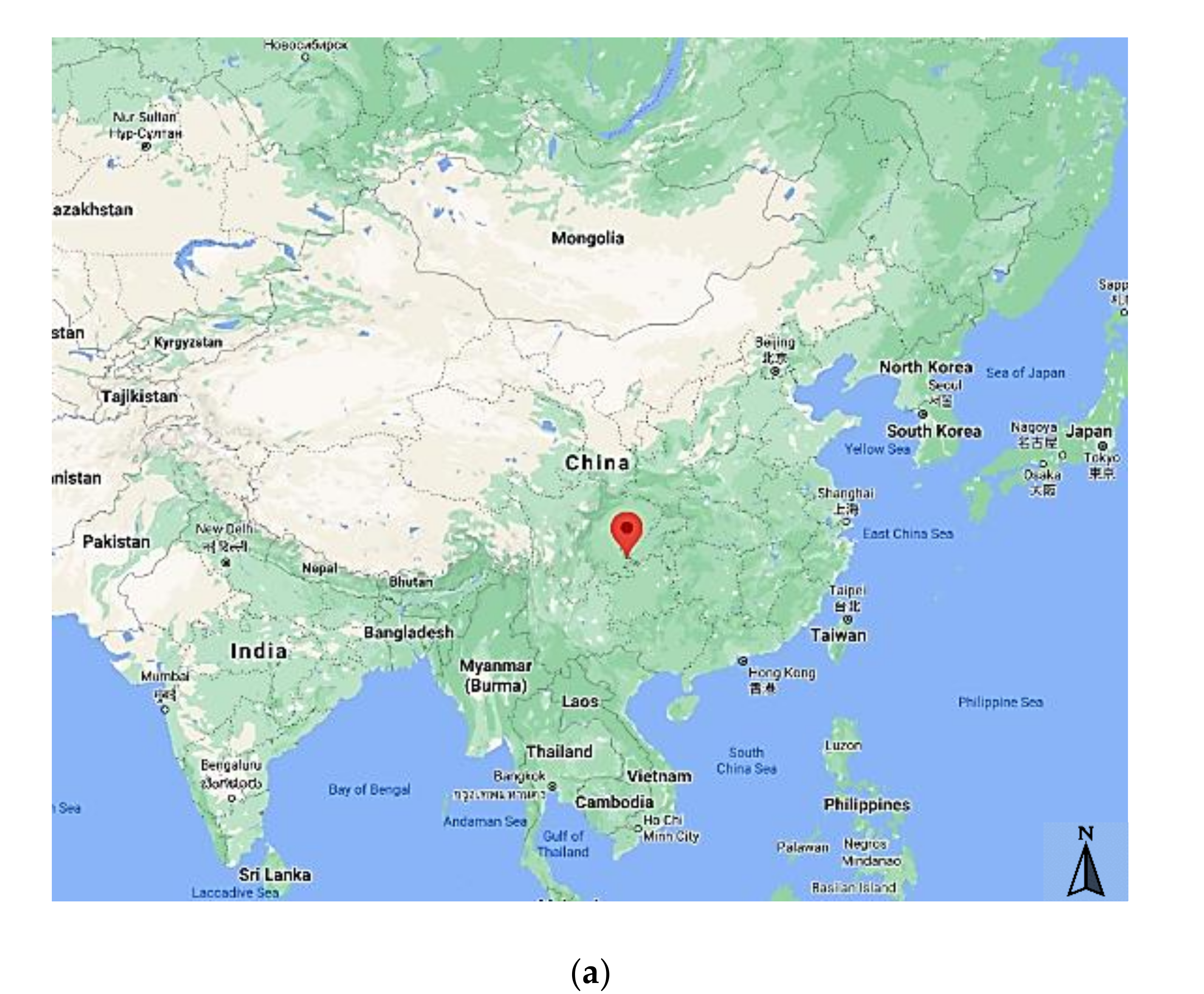
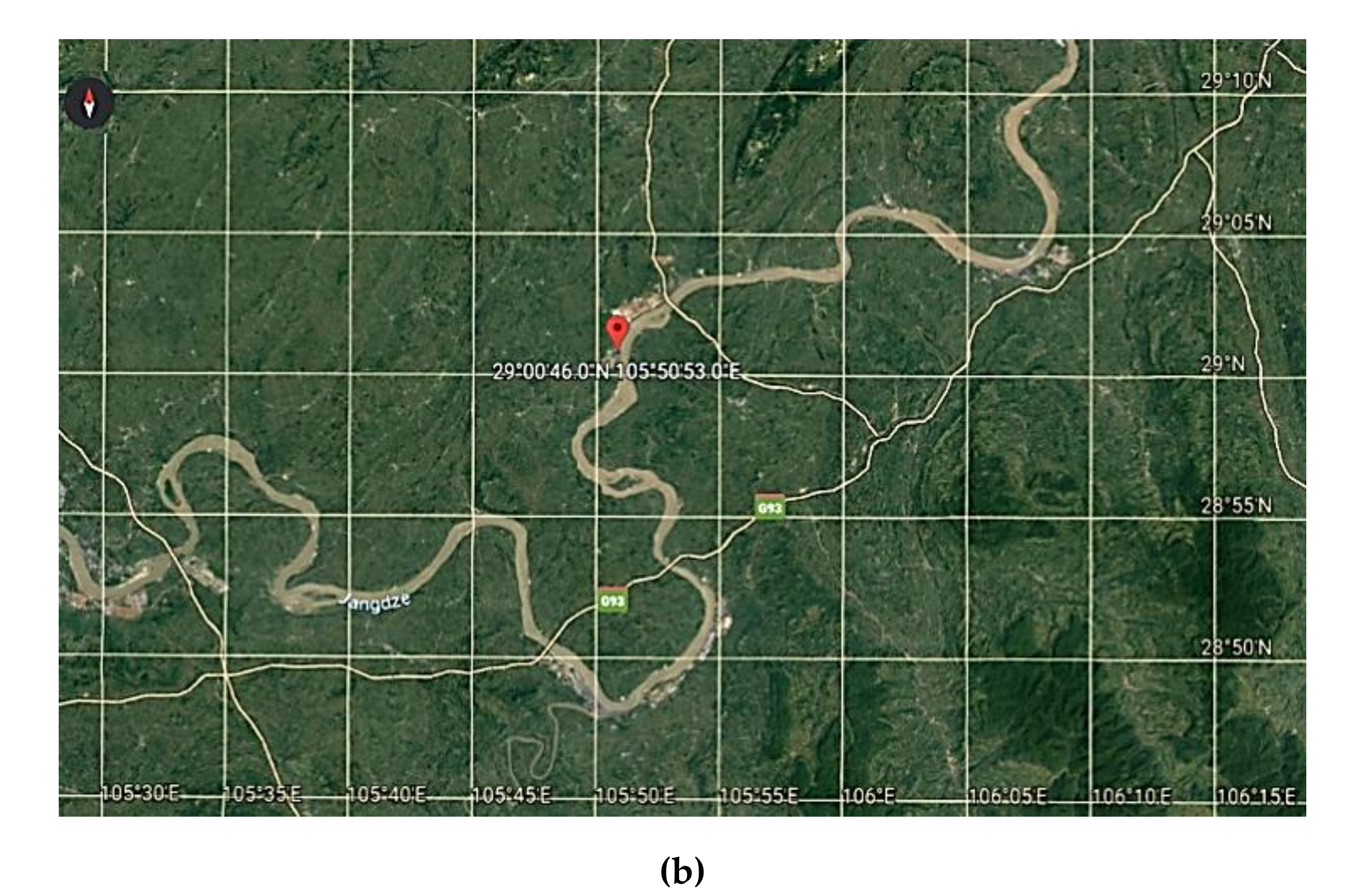
The Zhutuo Hydrological Station was built in April of 1954. It is located at 105°50′53′′ east longitude and 29°00′46′′ north latitude, in Zhutuo Town, Chongqing, China. Figure 2 is a map with the location of the study area. The Zhutuo Hydrological Station is a hydrological station in the upper reaches of the Yangtze River. Its observation range is from Hejiang County, Sichuan Province to Dazhong Village, Banan District, Chongqing City, covering a river section of 138.1 km and a catchment area of 694,725 km². The station is located at 2645 km from the mouth of the Yangtze River and at 145.4 km from Chongqing City.

3.2. Data Source

An experimental dataset was obtained from the repository of flow data recorded by Zhutuo Hydrological Station over the years. As the months of streamflow data of the three years from 1968 to 1970 were missing, there were 58 datasets available covering the period from 1954 to 2014. In this study, the months of streamflow data before 2014 were used as the training set to predict the months of streamflow data in 2014. The accuracy of the prediction model was analyzed by comparing the prediction data with the actual months of streamflow data and the predicted data yielded by fixed-window prediction method.

3.3. Model Simulation

The experimental dataset was divided into a training set and testing set. To prevent overfitting, the training set was further divided into training set and a validation set. Considering that the algorithm needs a long training time, simple validation was used in the experiment, that is, the validation set had only a fixed dataset. The first 54 months were used as the training set, the months from 2011 to 2013 were used as the validation set, and the months in 2014 were used as the testing set. Through trial and adjustment, the experimental parameters were set as follows: the network used a standard three-layer structure; the number of input nodes was the same as the size of the window; the number of output nodes was 1 (because predictive regression would be performed); the number of neural units in the hidden layer was 25; and the maximum number of iterations was 1500.

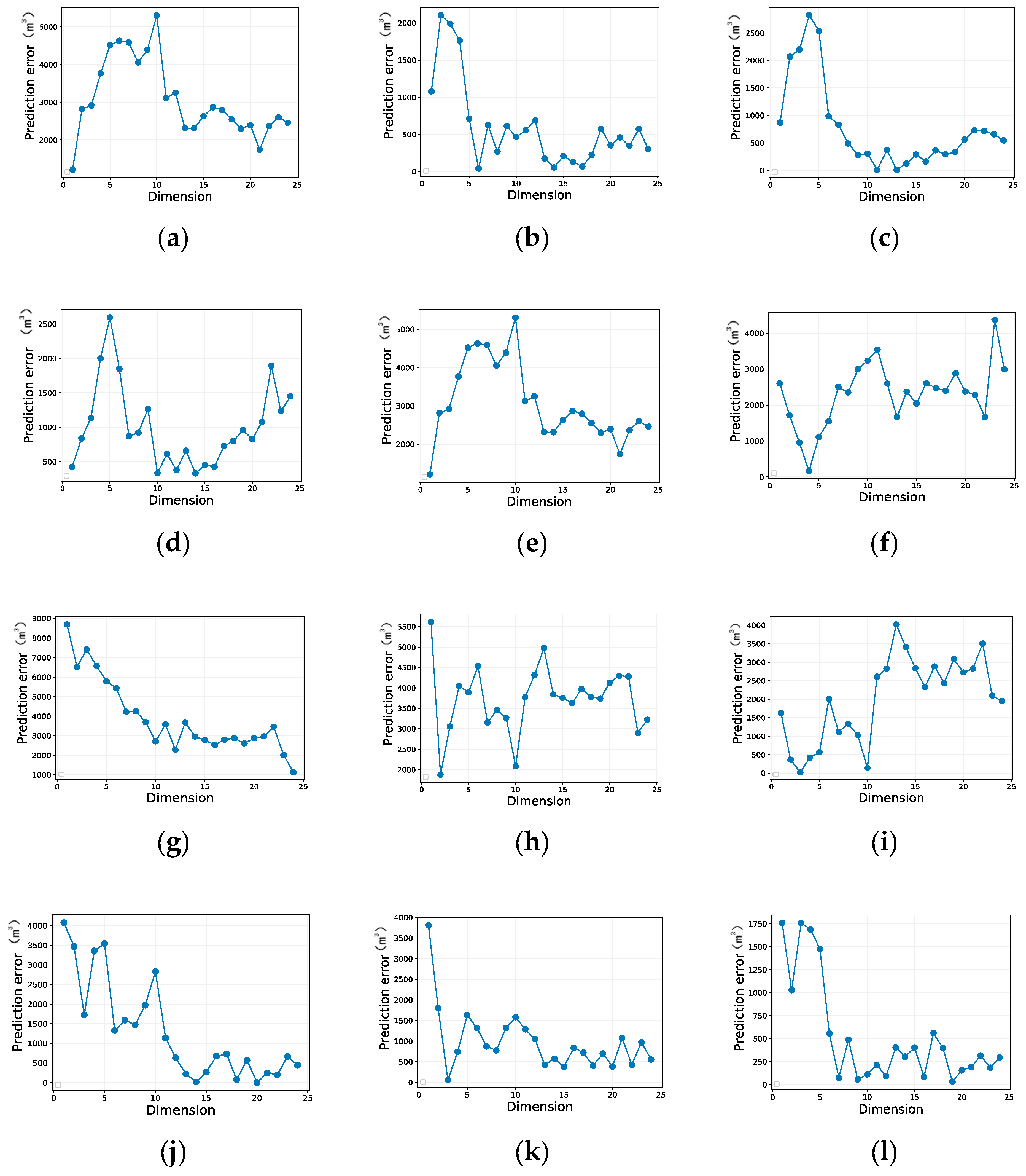
Figure 3 shows the sizes of the minimum error sliding windows (i.e., data dimension) from January to December were 22, 6, 11, 14, 1, 4, 24, 2, 3, 20, 3, and 19, respectively. The ordinate shows the error on the validation set. The prediction accuracy was better when the optimal window size was compared with the other window sizes. This difference was salient in the data of every month: the prediction error of the optimal window size could be hundreds of times smaller than that of the worst window size. This indicates that the proposed method has an advantage over the flow prediction method based on fixed sliding window.

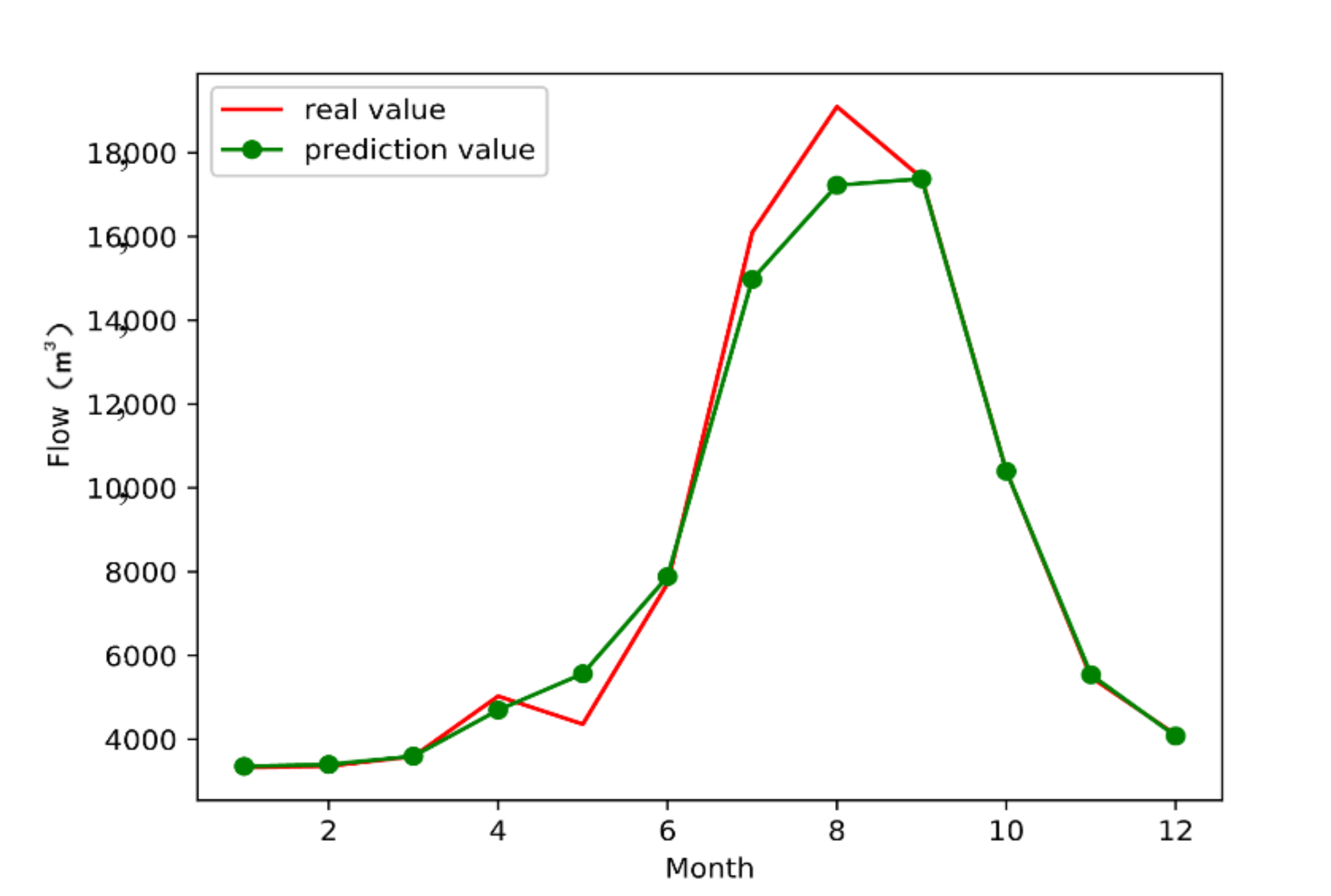
Figure 4 and Figure 5 show the flow prediction results in the Zhutuo Hydrological Station for the year 2014. It can be seen from Figure 4 that the prediction results yielded by the proposed method are in good agreement with the actual flow data. Among the errors shown in Figure 4, the prediction errors of almost all months are less than 10% except for May (which is 28.2%). For more than half of the months (i.e., January, February, March, June, September, October, November, and December), the prediction errors are less than 5%. These experimental results prove the effectiveness of the proposed method.

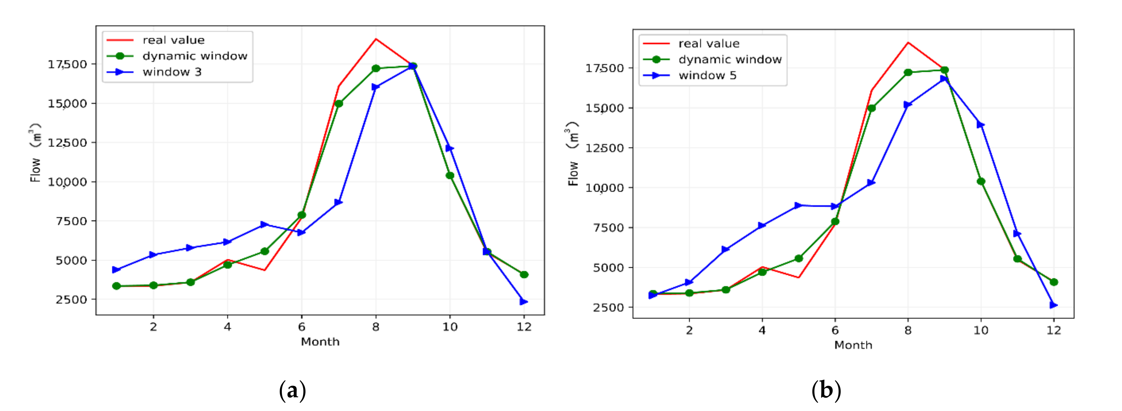
Figure 6a,b show the prediction results obtained when a dynamic window and fixed windows with sizes 3 and 5 were used. The optimization results of the dynamic window obtained through training and learning were closer to the actual data than those of the fixed window. The main reason for this is that the dynamic window method selects the optimal window for each month, meaning that it can better consider the differences in hydrological periodicity characteristics between months.

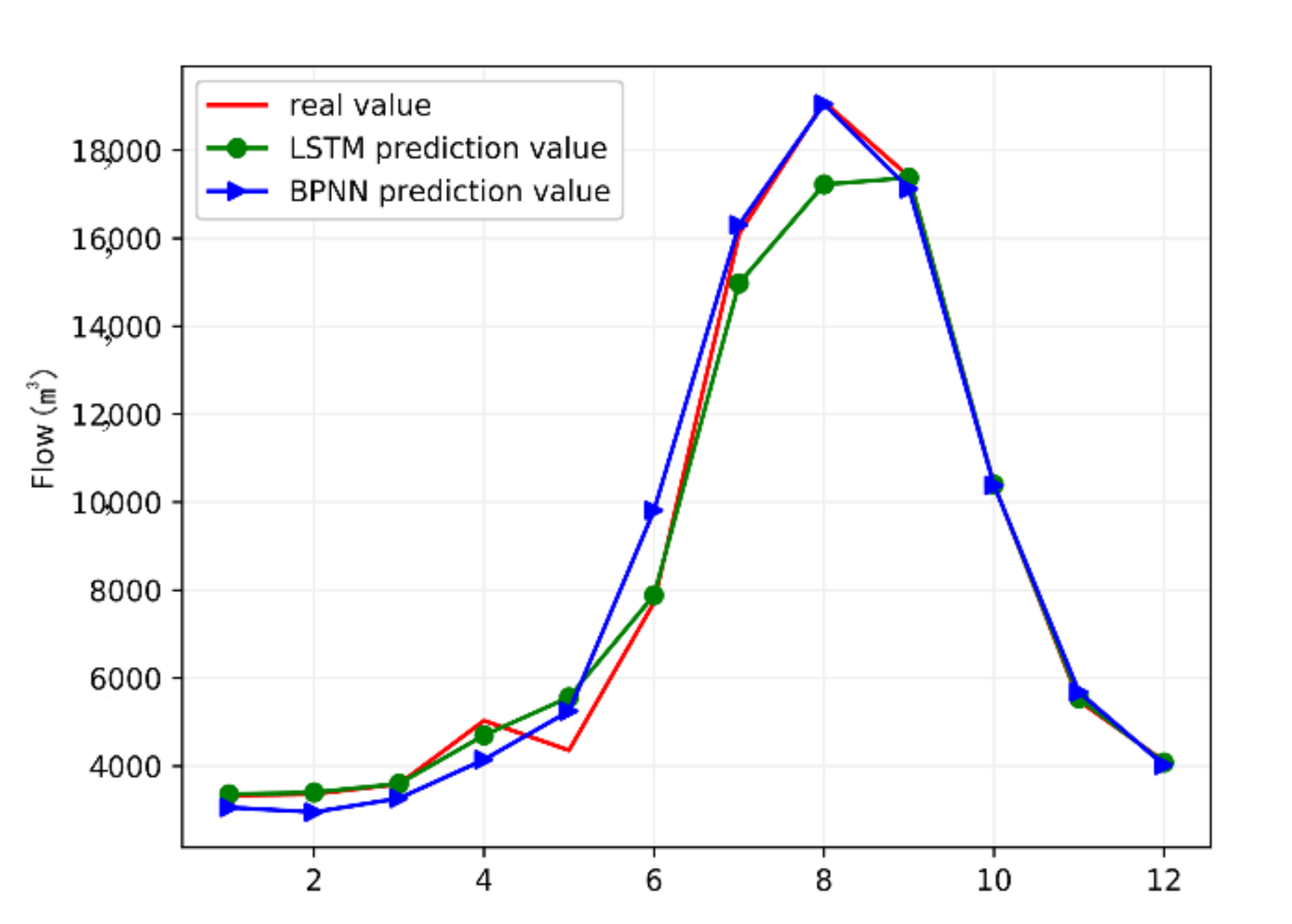
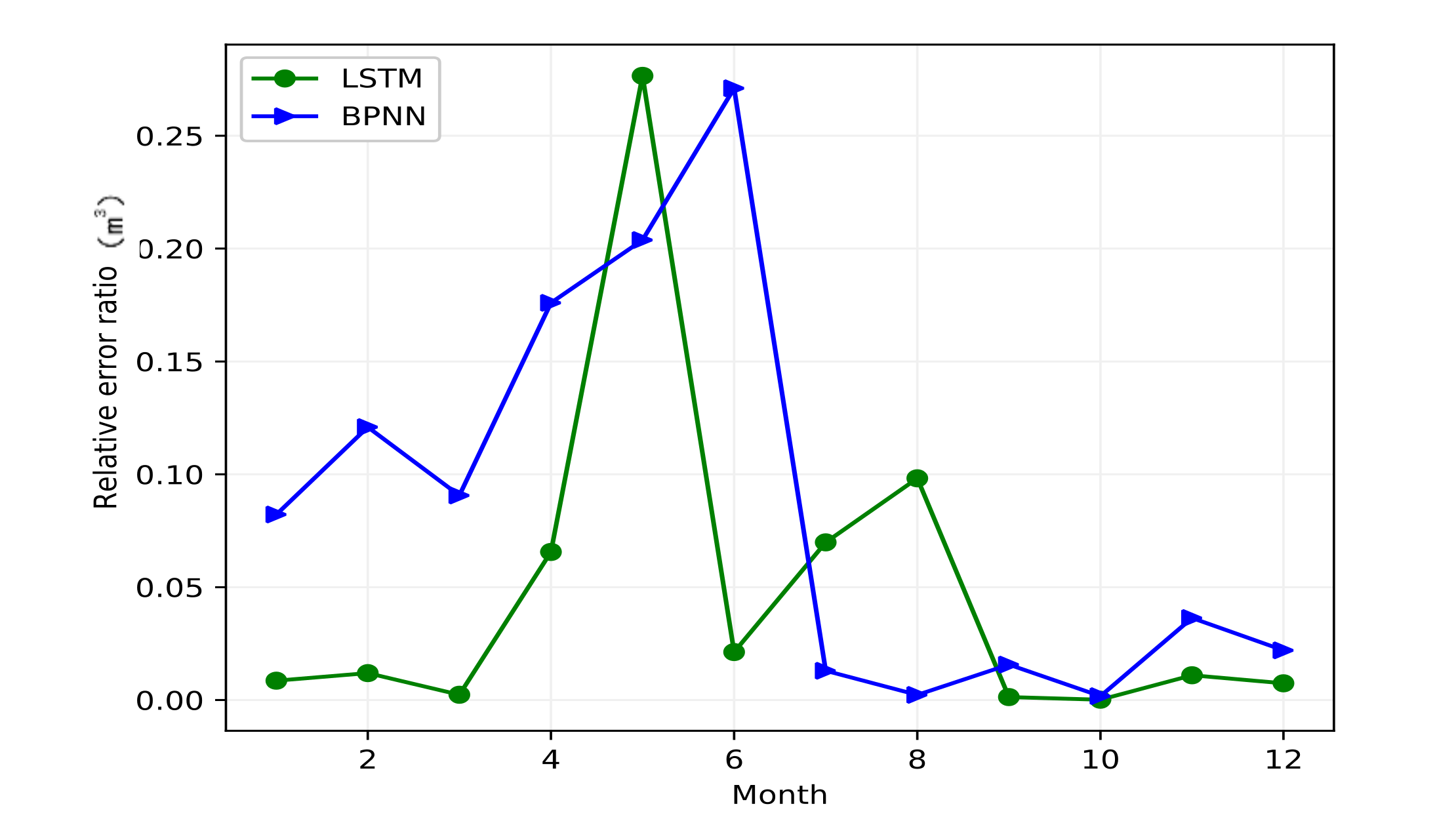
Figure 7 and Figure 8 show the flow prediction results in the Zhutuo Hydrological Station for the year 2014 yielded by the LSTM method based on the dynamic window proposed in this paper, and those yielded by the BP neural network method based on the dynamic window. It can be seen from Figure 7 that the prediction results yielded by the proposed method are in agreement with the actual flow data, except for July and August, for which the prediction results of the LSTM method were less accurate that those of the BP neural network method. The LSTM method yielded very accurate prediction results for the period from January to June. The error comparison in Figure 8 shows that, except for the three months of May, July, and August, the prediction errors produced by the dynamic window LSTM neural network in the remaining nine months were smaller than those produced by the dynamic window BP neural network. The average prediction error of LSTM was 4.78%, and the that of the BP neural network was 8.63%, indicating that the proposed method outperformed the dynamic sliding window BP neural network by 3.85%.

Despite the above advantages, while the new model is overall more accurate, it exhibited poorer accuracy in the high flow months (summer) compared to BP. The summer months are the ones with higher risk of flooding, and thus, from a risk management perspective, the BP model is likely more useful. The reason may be that the BP has a smaller number of parameters than LSTM, resulting in a better generalizability in processing unstable data. To combine the two advantages of the two algorithms to process the whole year’s data, two methods can be used: on the one hand, the dynamic BP is used in summer, and the dynamic LSTM is used in other seasons; on the other hand, to find a simple structure of the dynamic LSTM may be another effective way to make the dynamic LSTM fit with the summer season data.

4. Conclusions

This paper proposes a dynamic sliding window long-short term memory (LSTM) method for constructing flow data with optimal dimensions based on the timing and periodicity characteristics of streamflow data to remedy deficiencies in the existing fixed window method. To make a prediction for a certain month using this method, a LSTM verification prediction was performed on the data of 24 months before the month to be predicted first, and the months with the highest prediction accuracy were used as the optimal window dimension for the month to be predicted. Then, the dataset of the optimal window dimension was used to make a prediction. This method fully considers the difference in periodicity characteristics of hydrological data between different months. The results of verification using the data of the Zhutuo Hydrological Station showed that the proposed method achieved a higher average accuracy than similar fixed-window LSTM neural network methods do, i.e., by 3.85% compared with the sliding window back-propagation (BP) neural network method. However, the proposed method also has its deficiencies, as demonstrated by the 20% error in the flow prediction for the first month of the flood season. This is mainly because the prediction is based solely on historical flow data. If more meteorological factors affecting the flow are considered, then the proposed method is likely to yield a more accurate prediction result; in addition, if the clustering methods and feature selection methods can be combined into the proposed method, such as that in [33] and [34], the prediction performance may be further improved.

References

- Poff, N.L.; Zimmerman, J.K.H. Ecological responses to altered flow regimes: A literature review to inform the science and management of environmental flows. Freshw. Biol. 2010, 55, 194–205. [Google Scholar] [CrossRef]
- Loucks, D.P.; van Beek, E. Water Resources Planning and Management: An Overview. In Water Resource Systems Planning and Management; Springer: Cham, Switzerland, 2017. [Google Scholar] [CrossRef] [Green Version]
- Okewu, E.; Misra, S.; Maskeliunas, R.; Damaşeviçius, R.; Fernandez-Sanz, L. Optimizing green computing awareness for environmental sustainability and economic security as a stochastic optimization problem. Sustainability 2017, 9, 1857. [Google Scholar] [CrossRef] [Green Version]
- Pagano, T.C.; Wood, A.W.; Ramos, M.-H.; Cloke, H.L.; Pappenberger, F.; Clark, M.P.; Cranston, M.; Kavetski, D.; Mathevet, T.; Sorooshian, S.; et al. Challenges of Operational River Forecasting. J. Hydrometeorol. 2014, 15, 1692–1707. [Google Scholar] [CrossRef] [Green Version]
- Fotovatikhah, F.; Herrera, M.; Shamshirband, S.; Chau, K.W.; Ardabili, S.F.; Piran, J. Survey of computational intelligence as basis to big flood management: Challenges, research directions and future work. Eng. Appl. Comput. Fluid Mech. 2018, 12, 411–437. [Google Scholar] [CrossRef] [Green Version]
- Han, P.; Wang, X. Using ABCD model to predict the response of river basin hydrology to extreme climate. Yellow River 2016, 38, 16–22. [Google Scholar]
- Li, B.L.; Li, J.L.; Zan, M.J.; Li, Z.Q. R/S Grey Prediction of River Annual Runoff. Hydrology 2015, 35, 44–48. [Google Scholar]
- Zhu, B.; Zhao, L.L.; Li, M. Application of T-S-K fuzzy logic algorithm in Fuhe hydrological forecast. Hydrology 2015, 3, 53–58. [Google Scholar]
- Geng, Y.B.; Wang, Y.C. Prediction of river runoff variation based on BP neural network. Water Resour. Hydropower Northeast China 2016, 34, 29–30. [Google Scholar]
- Xing, B.F. Analysis of runoff prediction method based on wavelet neural network. Technol. Innov. Appl. 2012, 31, 41. [Google Scholar]
- Li, L. Application Research of BP Neural Network in Hydrological Data. Ph.D. Thesis, Shanxi University of Finance and Economics, Shanxi, China, 2011. [Google Scholar]
- Wang, L. Research on Runoff Forecast Based on BP Network. Ph.D. Thesis, Kunming University of Science and Technology, Kunming, China, 2015. [Google Scholar]
- Xingjian, S.H.I.; Chen, Z.; Wang, H.; Yeung, D.Y.; Wong, W.K.; Woo, W.C. Convolutional LSTM network: A machine learning approach for precipitation nowcasting. In Proceedings of the NIPS’15 28th International Conference on Neural Information Processing Systems, Montreal, QC, Canada, 8–13 December 2015; pp. 802–810. [Google Scholar]
- Wang, H.R.; Liu, X.H.; Tang, Q.; He, L. Support vector machine hydrological process prediction based on wavelet transform. J. Tsinghua Univ. Nat. Sci. Ed. 2010, 9, 1378–1382. [Google Scholar]
- Huang, Q.L.; Su, X.L.; Yang, J.T. Regression prediction model of daily runoff support vector machine based on wavelet decomposition. J. Northwest A F Univ. Nat. Sci. Ed. 2016, 44, 211–217. [Google Scholar]
- Sang, Y.F.; Singh, V.P.; Sun, F.; Chen, Y. Wavelet-Based Hydrological Time Series Forecasting. J. Hydrol. Eng. 2016, 21, 06016001. [Google Scholar] [CrossRef]
- Liu, H.Y.; Zhou, C.K. Prediction of the annual runoff of Guijiang River based on Markov chain. Trade News 2014, 50, 161. [Google Scholar]
- Sidekerskienė, T.; Woźniak, M.; Damaševičius, R. Nonnegative matrix factorization based decomposition for time series modelling. In Proceedings of the 16th IFIP International Conference on Computer Information Systems and Industrial Management (CISIM), Bialystok, Poland, 16–18 June 2017; pp. 604–613. [Google Scholar] [CrossRef] [Green Version]
- Sidekerskienė, T.; Damaševičius, R.; Woźniak, M. Zerocross density decomposition: A novel signal decomposition method. In Data Science: New Issues, Challenges and Applications; Springer International Publishing: Basel, Switzerland, 2020; pp. 235–252. [Google Scholar] [CrossRef]
- Xia, S.; Wang, G.; Chen, Z.; Duan, Y.; Liu, Q. Complete Random Forest based Class Noise Filtering Learning for Improving the Generalizability of Classifiers. IEEE Trans. Knowl. Data Eng. 2019, 31, 2063–2078. [Google Scholar] [CrossRef]
- Delafrouz, H.; Ghaheri, A.; Ghorbani, M.A. A novel hybrid neural network based on phase space reconstruction technique for daily river flow prediction. Soft Comput. 2018, 22, 2205–2215. [Google Scholar] [CrossRef]
- Ghorbani, M.A.; Khatibi, R.; Karimi, V.; Yaseen, Z.M.; Zounemat-Kermani, M. Learning from multiple models using artificial intelligence to improve model prediction accuracies: Application to river flows. Water Resour. Manag. 2018, 32, 4201–4215. [Google Scholar] [CrossRef]
- Yaseen, Z.M.; Fu, M.; Wang, C.; Mohtar, W.H.M.W.; Deo, R.C.; El-shafie, A. Application of the hybrid artificial neural network coupled with rolling mechanism and grey model algorithms for streamflow forecasting over multiple time horizons. Water Resour. Manag. 2018, 32, 1883–1899. [Google Scholar] [CrossRef]
- Fathian, F.; Mehdizadeh, S.; Kozekalani Sales, A.; Safari, M.J.S. Hybrid models to improve the monthly river flow prediction: Integrating artificial intelligence and non-linear time series models. J. Hydrol. 2019, 575, 1200–1213. [Google Scholar] [CrossRef]
- Meng, E.; Huang, S.; Huang, Q.; Fang, W.; Wu, L.; Wang, L. A robust method for non-stationary streamflow prediction based on improved EMD-SVM model. J. Hydrol. 2019, 568, 462–478. [Google Scholar] [CrossRef]
- Liang, C.; Li, H.; Lei, M.; Du, Q. Dongting Lake Water Level Forecast and Its Relationship with the Three Gorges Dam Based on a Long Short-Term Memory Network. Water 2018, 10, 1389. [Google Scholar] [CrossRef] [Green Version]
- Tian, Y.; Xu, Y.-P.; Yang, Z.; Wang, G.; Zhu, Q. Integration of a Parsimonious Hydrological Model with Recurrent Neural Networks for Improved Streamflow Forecasting. Water 2018, 10, 1655. [Google Scholar] [CrossRef] [Green Version]
- De Melo, A.G.; Sugimoto, D.N.; Tasinaffo, P.M.; Moreira Santos, A.H.; Cunha, A.M.; Vieira Dias, L.A. A new approach to river flow forecasting: LSTM and GRU multivariate models. IEEE Latin Am. Trans. 2019, 17, 1978–1986. [Google Scholar] [CrossRef]
- Meshram, S.G.; Ghorbani, M.A.; Shamshirband, S.; Karimi, V.; Meshram, C. River flow prediction using hybrid PSOGSA algorithm based on feed-forward neural network. Soft Comput. 2019, 23, 10429–10438. [Google Scholar] [CrossRef]
- Hochreiter, S.; Schmidhuber, J. LSTM can Solve Hard Long Time Lag Problems. In Proceedings of the Conference: Advances in Neural Information Processing Systems 9, NIPS, Denver, CO, USA, 2–5 December 1997. [Google Scholar]
- Pineda, F.J. Generalization of back-propagation to recurrent neural networks. Phys. Rev. Lett. 1987, 59, 2229–2232. [Google Scholar] [CrossRef] [PubMed]
- Hochreiter, S.; Schmidhuber, J. Long short-term memory. Neural Comput. 1997, 9, 1735–1780. [Google Scholar] [CrossRef]
- Xia, S.; Peng, D.; Meng, D.; Zhang, C.; Wang, G.; Giem, E.; Wei, W.; Chen, Z. A Fast Adaptive k-means with No Bounds. IEEE Trans. Pattern Anal. Mach. Intell. 2020, 1. [Google Scholar] [CrossRef]
- Xia, S.; Zhang, Z.; Li, W.; Wang, G.; Giem, E.; Chen, Z. GBNRS: A Novel Rough Set Algorithm for Fast Adaptive Attribute Reduction in Classification. IEEE Trans. Knowl. Data Eng. 2020, 1. [Google Scholar] [CrossRef]
Figure 1.
The structure of LSTM.
Figure 2.
The location of the Zhutuo Hydrological station: (a) overview and (b) zoom of study area.
Figure 3.
LSTM neural network prediction error curve of multidimensional data based on dynamic sliding window for 12 months in 2014. (a) January; (b) February; (c) March; (d) April; (e) May; (f) June; (g) July; (h) August; (i) September; (j) October; (k) November; (I) December.
Figure 4.
Comparison of flow prediction of Zhutuo Hydrological Station in 2014.
Figure 5.
The relative error ratio of the flow of Zhutuo Hydrological Station in 2014.
Figure 6.
2014 Zhutuo Hydrological Station Flow Error on the fixed window is 3 (a) and 5 (b).
Figure 7.
Prediction flow comparison of dynamic window LSTM and dynamic window BP neural network in Zhutuo hydrological station in 2014.
Figure 8.
Relative error ratio comparison of dynamic window LSTM and dynamic window BP neural network in Zhutuo hydrological station in 2014.
Publisher’s Note: MDPI stays neutral with regard to jurisdictional claims in published maps and institutional affiliations. |
© 2020 by the authors. Licensee MDPI, Basel, Switzerland. This article is an open access article distributed under the terms and conditions of the Creative Commons Attribution (CC BY) license (http://creativecommons.org/licenses/by/4.0/).
Share and Cite
MDPI and ACS Style
Dong, L.; Fang, D.; Wang, X.; Wei, W.; Damaševičius, R.; Scherer, R.; Woźniak, M. Prediction of Streamflow Based on Dynamic Sliding Window LSTM. Water 2020, 12, 3032. https://doi.org/10.3390/w12113032
AMA Style
Dong L, Fang D, Wang X, Wei W, Damaševičius R, Scherer R, Woźniak M. Prediction of Streamflow Based on Dynamic Sliding Window LSTM. Water. 2020; 12(11):3032. https://doi.org/10.3390/w12113032
Chicago/Turabian StyleDong, Limei, Desheng Fang, Xi Wang, Wei Wei, Robertas Damaševičius, Rafał Scherer, and Marcin Woźniak. 2020. "Prediction of Streamflow Based on Dynamic Sliding Window LSTM" Water 12, no. 11: 3032. https://doi.org/10.3390/w12113032
Note that from the first issue of 2016, this journal uses article numbers instead of page numbers. See further details here.