On the Use of Satellite Rainfall Data to Design a Dam in an Ungauged Site

Abstract

The estimation of the design peak discharge is crucial for the hydrological design of hydraulic structures. A commonly used approach is to estimate the design storm through the intensity–duration–area–frequency (IDAF) curves and then use it to generate the design discharge through a hydrological model. In ungauged areas, IDAF curves and design discharges are derived throughout regionalization studies, if any exist for the area of interest, or from using the hydrological information of the closest and most similar gauged place. However, many regions around the globe remain ungauged or are very poorly gauged. In this regard, a unique opportunity is provided by satellite precipitation products developed and improved in the last decades. In this paper, we show weaknesses and potentials of satellite data and, for the first time, we evaluate their applicability for design purposes. We employ CMORPH—Climate Prediction Center MORPHing technique satellite precipitation estimates to build IDAF curves and derive the design peak discharges for the Pietrarossa dam catchment in southern Italy. Results are compared with the corresponding one provided by a regionalization study, i.e., VAPI—VAlutazione delle Piene in Italia project, usually used in Italy in ungauged areas. Results show that CMORPH performed well for the estimation of low duration and small return periods storm events, while for high return period storms, further research is still needed.

1. Introduction

Peak flow estimation is of pivotal importance for the hydrological design of hydraulic structures. An incorrect evaluation can lead to the failure of the structures themselves. In the case of dams, the peak discharge is needed both for the design and for the evaluation of hydrologic safety of the structures. An underestimation of the design peak discharge could lead to overtop the dam due to insufficient drainage mechanisms [1,2]. Many of the approaches often adopted to define the design peak discharge for dams rely on historical discharge observations (e.g., [3,4,5,6]). However, due to the frequent lack of flow observations and thanks to the development of hydrometeorological models, the focus has moved on the estimation of the design storm, which is the one that gives rise to the design flood on the catchment [7]. Following this kind of approach, once the design storm is defined, a hydrological model is applied to estimate the corresponding peak flow. The rainfall–runoff models can be event-based, as in the case of the rational formula or the Natural Resources Conservation Service (NRCS) method [8], or based on continuous simulations [9,10]. One of the most common approaches adopted is the event-based one, with the design storm being associated to a certain return period $T_R$, usually provided by national guidelines. The intensity of the design storm for a fixed $T_R$ and duration is defined through mathematical relationships that quantify the rainfall intensity of storms with specific probability of occurrence at changing durations, known as intensity–duration–frequency (IDF) curves [8] and intensity–duration–area–frequency (IDAF) curves [11]. IDF and IDAF curves differ in the spatial scale of the information they provide; the former give a punctual rainfall intensity, whereas the latter provide an areal intensity estimate. As precipitation is highly variable in space and time, uncertainties in the definition of rainfall intensity at a catchment scale through IDF curves arise [12]. IDAF curves are therefore needed when the design storm over an area is required, as for the case of the design of a dam.

The rain-based approaches to derive the design peak discharge rely on the use of precipitation records collected from rain gauges. Although rain gauge observations are more common than flow records, some rural areas of the world, where it is more likely that new dams are built, are still poorly gauged or totally ungauged [13]. In any case, rainfall monitoring networks in general have been declining over the last several decades due to their high maintenance and operating costs [14].

In the case of completely ungauged basins, it is common to build the IDF/IDAF curves using the parameters determined with previous regional studies, if any exist for the case study area, or to consider the IDF/IDAF curves defined for gauged watersheds belonging to the same homogeneous region or with similar climatic and topographic characteristics of the case study, according to the spatial proximity and physical similarity principles, respectively [15].

However, in many regions around the globe, the lack of a rainfall monitoring network makes the development of regionalization methods an impossible task. In this regard, a unique opportunity is provided by satellite rainfall data. Many satellite precipitation products have been developed in the last two decades, with different spatial (i.e., from 4 to 25 km) and temporal (i.e., from 30 min to monthly) resolutions, with a quasi-global coverage. Among all the satellite products, the most frequently employed in hydrologic applications are the following. The CMORPH—Climate Prediction Center MORPHing technique [16], which combines data from geostationary infrared and passive microwave satellites to provide rain rate estimates at a squared grid of 8 km with 30-min time resolution, from 1998 to the present; PERSIANN—Precipitation Estimation from Remotely Sensed Information using Artificial Neural Networks [17], which provides precipitation rate on a squared grid of 0.25° from an infrared brightness temperature image given by geostationary satellites, with different time resolution (i.e., from hourly to monthly, and temporal availability, ranging from 1983 for the monthly scale and from 2000 for the hourly scale to the present); TMPA—Tropical Rainfall Measuring Mission Multi-satellite Precipitation Analysis [18], which combines data coming from multiple satellites to produce rainfall estimates on a squared grid of 0.25° with a three-hour time scale for the period 1998–2015; CHIRPS—Climate Hazards Group Infra-Red Precipitation with Station data [19], which incorporates infrared satellite imagery with in situ data to produce precipitation estimates on a squared grid of 0.05° on a daily scale from 1981 to the present. Although satellite precipitation estimates are available for remote and ungauged areas, their time series are usually short and their accuracy varies with the precipitation type, topography, and climate of the region [20].

Satellite precipitation estimates have so far employed for many hydrological applications, such as to model rainfall–runoff [21], to capture precipitation [22,23] and heavy rainfall events [20], and to create IDF curves [12,24], but they have never been adopted to compute design discharge for a hydraulic structure. This paper evaluates, for the first time, the performances of satellite observations on the design of a hydraulic structure. This assessment can be extremely useful when applied to ungauged areas whereby the satellite estimates represent the sole opportunity to design a hydraulic structure, e.g., dam. Therefore, here, we compare the values of IDF/IDAF curves and design flow peaks obtained using satellite precipitation estimates and using parameters from a previous regionalization study [25] which is usually adopted in an ungauged or poorly gauged area in Italy. The main purpose is to quantify the difference between the two data sources in order to verify if the use of satellite precipitation employed to evaluate the design storm, and thus design discharge, can be a valid alternative in ungauged areas where no regionalization studies are actually available. The study method is applied to the Pietrarossa dam catchment, located in Sicily, southern Italy. As to build IDFs/IDAFs, long time series with fine temporal scale, at least hourly, are required; the satellite data set hereby employed is the set of CMORPH rain rate estimates, which provides the longest time series at the lowest time resolution, i.e., 30 min. To quantify the effect of the use of different rainfall data sets from a more practical perspective, we compute the dimension of the spillway needed to ensure the hydrological safety of the dam in the two analysed cases. The paper is organized as follows: in Section 2, we provide information about the case study and data employed; in Section 3, we introduce the methods adopted to first evaluate the satellite performances, to compute the design flood peak and to determine the dimensions of the spillway; in Section 4, we present the results, and we discuss it in Section 5; in Section 6, we draw the conclusions.

2. Study Area and Data

2.1. Study Area

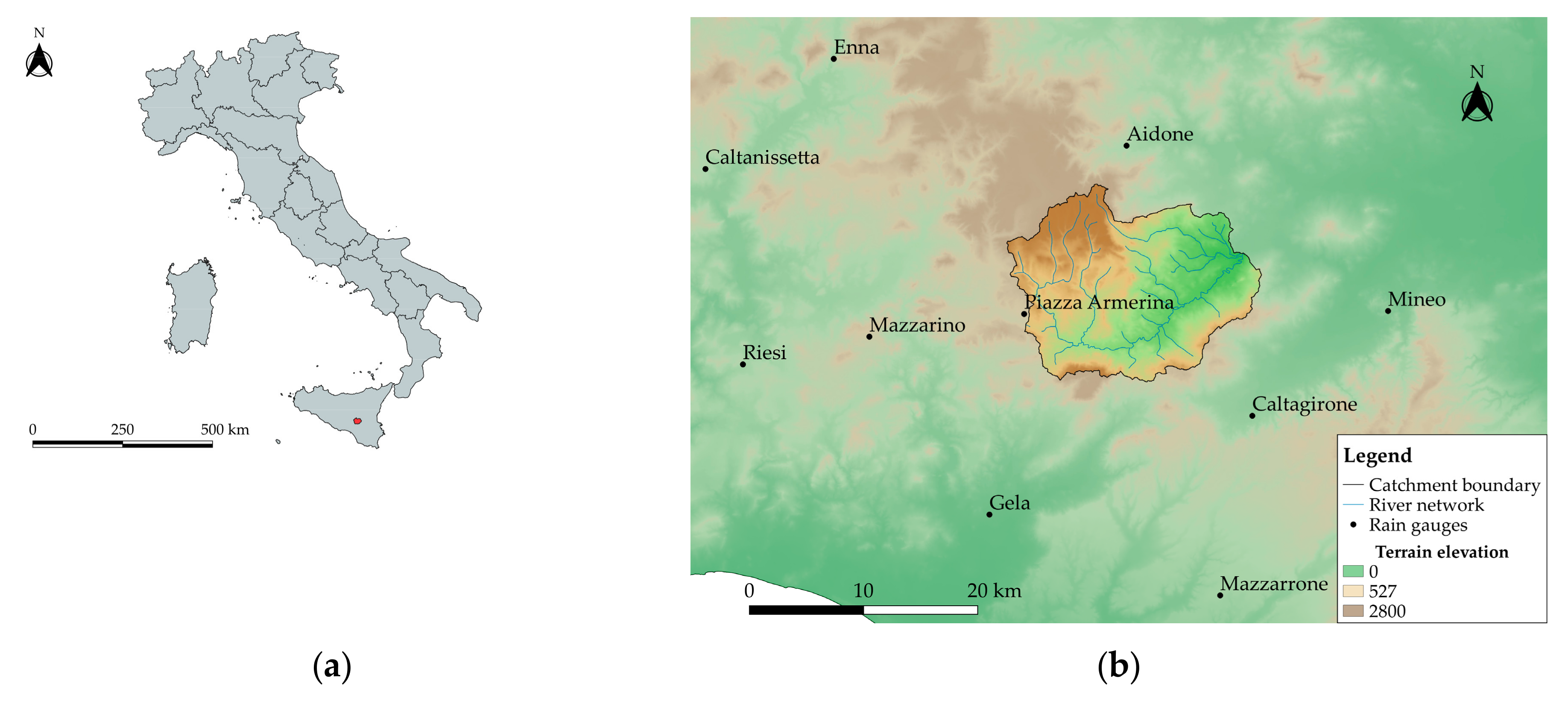
The Pietrarossa dam is located in the central-eastern part of Sicily, the biggest island of Italy (Figure 1a). It is located at the confluence of Acquabianca and Pietrarossa rivers, which merge after the dam into the Margherito river. The dam construction started in 1989 with the main purpose of irrigating the agricultural fields in the southern part of the Simeto catchment. However, only a few years later, the construction was interrupted due to the discovery of archaeological remains of the Roman era [26]. The structure is nowadays complete for the 97%, with the main structure in the rock-fill, intake tower, and spillways already completed. The dam drains an area of 257 km², which from now on will be referred as the Pietrarossa catchment. The dam was built on a plan with average altitude of 170 m a.s.l. and it was designed to have a capacity of 32 millions m³, corresponding to the maximum water level of 188 m a.s.l. The Pietrarossa catchment is located in the inner hilly area of the island (Figure 1b) and it is characterized by a mean yearly precipitation of 485 mm, which is below the corresponding mean regional value of 600 mm. Precipitation occurs mostly during autumn and winter seasons (September to March).

For this study, precipitation observations from the regional rain gauge network and from the CMORPH satellite product are employed. It has to be noted that there are two different available ground-based networks in Sicily, one managed from Servizio Informativo Agrometeorologico Siciliano (SIAS) and one from Osservatorio delle Acque. Although the latter was established in the 1920s and was used to conduct the regionalization study used as a benchmark in this work, many of the stations were dismantled in the last two decades, i.e., the period of satellite observations availability. In order to have both rain gauge and satellite observations referred to the same period, in this work, we employed the data provided by SIAS.

2.2. Precipitation Data Sets

The ground-based data set consists in the 10-min resolution precipitation time series provided by the tipping bucket rain gauges of the SIAS. The observations are available with a minimum resolution of 0.2 mm for the period 2002–2017, even though with discontinuities for some stations. Because of the lack of monitoring stations within the catchment and also to have a better understanding of the CMORPH performance in the whole area surrounding the case study, we consider all the recording rain gauges located within 40 km of distance from the barycentre of the watershed, for a total of 12 stations.

The Climate Prediction Center MORPHing (CMORPH) precipitation, selected for the case study, has been developed by the National Oceanic and Atmospheric Administration (NOAA) Climate Prediction Center (CPC) to provide precipitation rate estimates on a quasi-global scale (60° N–60° S), combining geostationary satellite infrared (GEO IR) consecutive images and passive microwave (PMW) precipitation rate estimates [16]. Full-resolution IR satellites provide global surface/cloud-top temperature consecutive images on a regular squared grid of 0.03635° of latitude and longitude resolution (~4 km at the equator), every 30 min. The IR images are adopted to derive cloud motion vectors through the cross-correlation technique. In the meantime, an ensemble of low-Earth-observations (LEO) PMW satellites provide rain rate estimates with 30-min time resolution on regular grids with spatial resolution varying according to the satellite, ranging from 4.6 to 15 km. To take into account all the spatial scales of the different input data, the 0.0727° latitude and longitude (8 km at the equator) grid resolution was selected as the definitive grid. To produce the global rate field, PMW estimates are then mapped to the nearest point of the 8 km grid and for the locations where no PMW estimates are available, cloud motion vector is adopted to propagate in time, in the backward and forward direction, the PMW information. More details about the specific of satellites and methodology adopted to derive CMORPH can be found in [16,27].

The technique just described is employed to produce the CMORPH version 0.X, which is given on a grid with 8 km × 8 km spatial resolution and with 30 min of temporal resolution. Version 0.X has been improved by bias correction to generate the version 1.0 [27], which is available with same spatial and temporal resolution of version 0.X for the period 1998–present. A third CMORPH version is also available, which is the bias corrected product blended with the daily gauge analysis [28], only available on a 0.25° grid. For our study, both the fine spatial and temporal scale are required, therefore CMORPH 1.0 is employed, since it proved to give good performances at a fine spatial and temporal scale [29].

2.3. Data Pre-Processing

CMORPH provides rain rate estimates every 30 min, while the rain gauges give rainfall depth observations every 10 min. Due to the differences in the two data sets, some preliminary operations are therefore needed. First of all, rain gauge time series are aggregated at the 30-min scale, to be consistent with CMORPH temporal resolution. Second, satellite rain rate estimates are transformed into precipitation depths, multiplying each record for the corresponding time interval ∆t = 0.5 h. Third, CMORPH time series are filtered out to match the rain gauge minimum resolution of 0.2 mm: each satellite record lower than 0.2 mm is set to 0 mm. Finally, a quality control on the missing data for both data sets is performed. Only the stations and the pixels having time series with less than 20% of missing observations are considered. Two rain gauges are excluded from the data set as a consequence of the quality control, while all the satellite pixels are selected. The filtered precipitation data provided by CMORPH and rain gauges were then aggregated also to the daily scale, to check the performance of satellite observations at different time scales (see Section 3.1).

3. Methodology

In the hydrological design of dams, spillway dimensions are calculated based on the flood peak associated to a fix return period [30], which is evaluated via frequency analysis of the historical observations. The traditional approaches for the estimation of frequency analysis are mainly two, one relying on flow observations and the other on precipitation records [10]. River flow observations are often not available; thus, in this work, we adopt the second of the two approaches, following a commonly used procedure to derive peak discharges in ungauged catchments, i.e., the rational method. It consists mainly in two steps: first, determine the design storm for the catchment, for fixed durations and return periods, using the intensity–duration–area–frequency (IDAF) curves; second, determine design peak flow associated to the critical rainfall intensity using the rational formula.

The methodology can be thus summarized in three macro-steps: first, we compare the goodness of satellite observations against the ground-based ones by computing several continuous and categorical evaluation indexes; second, we evaluate the design storm for different return periods, using intensity–duration–area–frequency (IDAF) curves built both with satellite observations and the parameters provided by a previous regionalization study, i.e., VAPI—VAlutazione delle Piene in Italia (flood evaluation in Italy) project [31]; last, we compute the design flood peak for the catchment and we determine the spillway dimensions as an applicative example. Further details are provided in the following subsections.

3.1. Evaluation Indexes

Satellite precipitation estimates are affected by random and systematic errors, commonly referred to as bias. Their accuracy is usually lower than that of rain gauge observations, since satellites provide indirect estimates of precipitation, coming from IR and PWR satellites [32,33]. Even though previous studies [20,23,34] evaluated CMORPH skills in capturing rainfall, a universal assessment cannot be done, since performances change with the precipitation type, topography, climate of the region [20] and temporal resolution [22]. Although the length of the available time series of rain gauges does not allow for a reliable estimate of the IDAF curves, it is sufficient to estimate the CMORPH capacities in precipitation capture [20,22,23].

In this study, a point–pixel evaluation is performed (e.g., [33,35], meaning that each punctual time series recorded by a rain gauge is directly compared against the areal satellite observations referred to the grid pixel where the rain gauge is located. It differs from the so-called pixel–pixel comparison because in the latter, areal rainfall observations are compared. As precipitation observations coming from rain gauge are punctual, they first need to be transformed into areal rainfall. The conversion is usually done by interpolation of gauge data on a regular grid, with finer spatial resolution than the one of the reference satellite data. All the interpolated information belonging to the same pixel of the reference grid are then averaged to create the areal precipitation needed. Although there is a scale mismatch between point rainfall measured by rain gauges and areal precipitation detected by satellite [23], the point–pixel comparison is preferred over the pixel–pixel comparison to avoid introduction of interpolation bias caused by the low density of the ground-based network [34,36].

The point–pixel comparison is conducted by the computation of some categorical and continuous statistical metrics, as commonly done in previous literature works [22,23,33,37,38]. The employed continuous indexes give information about the bias and correlations between satellite and rain gauge observations. They are the mean absolute error (MAE), the root–mean–squared error (RMSE), the normalized standard error (NSE), the correlation coefficient (CC), and the mean bias error (MBE). The categorical metrics only distinguish two conditions, i.e., rain or no rain, but they do not quantify the differences in terms of mm between the two data sets. The ones hereby adopted are the probability of detection (POD), which represents the fraction of events correctly detected by satellite, the false alarm ratio (FAR), which gives the fraction of events detected by satellite but not observed by rain gauges, and the critical success index (CSI), which provides the overall performance of the satellite product. A list of the metrics computed is given in

Table 1. List of statistical metrics computed. The values marked in bold stand for perfect match between satellite and rain gauge observations. $S_i$ stands for the i-th satellite estimation, $R_i$ is the corresponding rain gauge observation, $N$ is the number of observations available for the station, $H$ stands for the number of times that both CMORPH and rain gauges detected rainfall, $M$ represents the number of times rainfall is observed in a rain gauge but it is not detected by the satellite product, $F$ gives the number of times precipitation is not observed in a rain gauge but it is detected by CMORPH, $cov\left(S,R\right)$ is the covariance between rain gauge and CMORPH time series, $\sigma \left(S\right)$ and $\sigma \left(R\right)$ are the standard deviation of satellite and rain gauge time series, respectively.

Statistical Metric	Symbol	Equation	Range of Values	Unit
Mean Absolute Error	MAE	$\frac{1}{N}{\displaystyle {\displaystyle \sum }_{i=1}^N}\left|S_i-R_i\right|$	$\left[\mathbf{0},+\infty \right)$	mm
Root Mean Squared Error	RMSE	$\sqrt{\frac{1}{N}{\displaystyle {\displaystyle \sum }_{i=1}^N}{\left(S_i-R_i\right)}^2}$	$\left[\mathbf{0},+\infty \right)$	mm
Normalized Standard Error	NSE	$\frac{\sqrt{\frac{1}{N}{{\displaystyle \sum }}_{i=1}^N{\left(S_i-R_i\right)}^2}}{\frac{1}{N}{{\displaystyle \sum }}_{i=1}^N{R}_i}$	$\left[\mathbf{0},+\infty \right)$	-
Mean Bias Error	MBE	$\frac{{{\displaystyle \sum }}_{i=1}^N{S}_i-R_i}{{{\displaystyle \sum }}_{i=1}^N{R}_i}·100$	$\left[\mathbf{0},+\infty \right)$	-
Correlation Coefficient	CC	$\frac{cov\left(S,R\right)}{\sigma \left(S\right)·\sigma \left(R\right)}$	$\left[-1,\mathbf{1}\right]$	-
Probability of Detection	POD	$\frac{H}{H+M}$	$\left[0,\mathbf{1}\right]$	-
False Alarm Ratio	FAR	$\frac{F}{F+M}$	$\left[\mathbf{0},1\right]$	-
Critical Success Index	CSI	$\frac{H}{H+F+M}$	$\left[0,\mathbf{1}\right]$	-

, together with their range of values. In Table 1, for each of the indexes computed, the value which means a perfect match between satellite and rain gauge records is marked in bold.

In addition, scatter plots between ground-based and satellite-based observations are also computed for each station. Scatter plots are built considering only the records for which both rain gauges and CMORPH detected rain. All the evaluation indexes are computed both on the 30-min and daily time series.

3.2. Intensity–Duration–Area–Frequency (IDAF) Curves

Intensity–duration–area–frequency (IDAF) curves provide a mathematical relationship to link the intensity of rainfall over an area and fixed duration to its probability of occurrence. They represent the spatial extension of the intensity–duration–frequency (IDF) curves [39]. IDAFs are built to define the characteristics of the design storm at a catchment scale, as required for the design of many hydraulic structures, such as dams. In this work, IDAFs are built adopting two different methods, one for each data set employed. The use of two different procedures is due to the differences in the two data sets, since satellite observations provide areal precipitation estimates while the VAPI approach gives punctual rainfall estimates.

3.2.1. VAPI Regionalization Approach

Extreme daily and sub-daily precipitation has been studied in Italy by the VAPI—VAlutazione delle Piene in Italia (floods evaluation in Italy) project, which applies a regional frequency analysis (RFA) approach to produce a robust statistical analysis of rainfall in the country. According to the results obtained for Sicily [25], extreme precipitation in the region can be described by the two components extreme value (TCEV) distribution to take both the usual and the extreme values of rainfall into account. The regionalization procedure is hierarchical and it is made out of three different levels to evaluate the parameters of the TCEV distribution. At the end of it, three homogeneous areas are identified in the region. The value of rainfall depth $h\left(d,T_R\right)$, referred to a fixed duration $d$ and return period $T_R$, can be evaluated using the relationship proposed by Cannarozzo et al. [25] in the VAPI project and commonly used in Italy (e.g., [31,40,41,42,43]):

$$h\left(d,T_R\right)=h’\left(d,T_R\right)·{\mu }_R\left(d\right)$$

(1)

The term $h’\left(d,T_R\right)$ is the dimensionless rainfall of duration $d$ and return period $T_R$, also known as “growth factor”, and the term ${\mu }_R\left(d\right)$ is the mean rainfall depth for a fixed duration. It has been shown by Cannarozzo et al. [25] that the growth factor can be computed using a mathematical relationship that varies with the homogeneous sub-region. The same authors also provide three empirical relationship found for each homogeneous sub-region of Sicily. In our case, the study area belongs to the sub-region C and the growth factor is computed with the following:

$$h^{\prime }\left(d,T_R\right)=0.5015-0.003516 d+\left(0.0003720 d^2+0.00102 d+1.1014\right)\log T_R$$

(2)

Ferrari et al. [31] and Cannarozzo et al. [25] showed that the factor ${\mu }_R\left(d\right)$ depends only on the duration of the rainfall event and they propose the following power law for its evaluation:

$${\mu }_R\left(d\right)=a d^n$$

(3)

where the parameters $a$ and $n$ are constant for each time series. The VAPI project provides the values of $a$ and $n$ for all the stations employed in the study, together with maps of iso-$a$ and iso-$n$ to derive the parameters at ungauged locations. For the case study, parameters $a$ and $n$ are the mean values of parameters $a$ and $n$ available for the stations surrounding the catchment [44].

Dividing both terms of Equation (1) for the duration of the rainfall event, we obtain the expression of IDF curves given by the regionalization approach:

$$i\left(d,T_R\right)=i’\left(d,T_R\right)·{\mu }_R\left(d\right)$$

(4)

The values of rainfall intensity obtained following this procedure is a punctual intensity, however for the design of hydraulic structures the rain intensity over the catchment, provided by IDAF curves, is needed. Due to the high variability of precipitation characteristics over space and time, approximating precipitation over a catchment using only one rain gauge, i.e., punctual observations, can lead to limitations [45,46,47]. The effective rain intensity (or depth) over the watershed is usually computed by multiplying the punctual intensity, given by IDF curves, for the Areal Reduction Factor (ARF). The ARF is a corrective coefficient, in the range (0,1), defined as the ratio between areal average rainfall and point rainfall. Many methods to compute ARF have been proposed in literature, including empirical formulations and approaches based on rainfall observations [48]. Since no previous studies about the ARF for the study area are available, the empirical formulation proposed by Koutsoyiannis and Xanthopoulos [49] is adopted. According to the authors, the ARF depends only on the duration $d$ of the storm event and on the area $A$ of the catchment, following the rule:

$$ARF\left(A,d\right)=1- \frac{0.048·A^{0.36-0.01 \ln \left(A\right)}}{d^{0.35}}$$

(5)

where area $A$ is expressed in km² and the duration $d$ in hours.

Once the ARF is computed for the catchment area, i.e., 257 km², and for the fixed durations of 1, 3, 6, 12 and 24 h, the IDAF curves are built by multiplying IDF curves obtained with the regionalization approach (Equation (4)) and the ARF factor, as follows:

$$i \left(A,d,T_R\right)=i\left(d,T_R\right)·ARF\left(A,d\right)$$

(6)

3.2.2. CMORPH Observations

The CMORPH rainfall estimates are the average precipitation observed in each 8 km × 8 km cell of the domain. For this reason, IDAFs are developed via frequency analysis of mean areal precipitation depths over different durations, with no need for further corrections as in the case of punctual rainfall observations (see Section 3.2.1). The time series of areal precipitation required are evaluated with a weighted average of the precipitation estimates of all the cells of the satellite grid falling within the watershed boundaries. The weights of the average are the Thiessen coefficients [50], as expressed by the following:

$$h_A= {\displaystyle \sum }_{i=1}^N{h}_i· {\lambda }_i={\displaystyle \sum }_{i=1}^N{h}_i· \frac{A_i}{A}$$

(7)

In Equation (7), $h_A$ is the mean areal precipitation depth over the catchment, $h_i$ is the precipitation depth for the i-th cell in the catchment, $A_i$ is the area of influence for the i-th cell, ${\lambda }_i$ is the Thiessen coefficient for the i-th cell, $N$ is the total number of cells for the catchment, $A$ is the total watershed area, i.e., 257 km².

Once that the areal precipitation time series are obtained, the frequency analysis to derive IDAF curves is performed. First, the Annual Maxima Series (AMS) is built: for each year of records we select the maximum value of precipitation depth obtained for the fixed durations of 1, 3, 6, 12 and 24 h. Second, we use the method of moments proposed by Pearson [51] to fit the statistical model to the samples of maxima. Extreme rainfall in Sicily has been previously described by Two-Component Extreme Value (TCEV) probability distribution [25,41], however it is well known that, as TCEV distribution is defined by four parameters, long samples of data are needed to have a robust estimate [52]. As in our case study samples are of limited length, we selected as possible statistical models the Extreme Value (EV) distribution types I and II, also known as Gumbel and Fréchet distributions respectively, as widely suggested in literature for this kind of analysis (e.g., [53,54]). To detect the best fitting distribution, the norm N1 test [55] is then performed.

Finally, the IDAF curves are derived for the return periods of 20, 50, 100, 500, 1000, 2000 and 3000 years. We are aware that the limited length of observations is not sufficient to produce robust rainfall statistical estimates for high return periods. However, the aim of this work is to reproduce the situation of completely ungauged areas, where reliable regionalization studies are not available or cannot be developed due to the lack of precipitation observations [12,56], and to evaluate the potentiality and the value of satellite products, with all their limits, in those areas.

The IDAFs are built using a simplified version of the power law proposed by Bernard [57] and widely used in hydrology (e.g., [53,58]):

$$i=b t^{m-1}$$

(8)

where $i$ is the rainfall intensity, $t$ is the duration of the rainfall event, $b$ and $m$ are the parameters of the curves, which are calibrated according to the sample data. The parameter $b$ depends on the return period and on the probability distribution selected, while $m$ is the same for all the curves and can assume values in the range (0, 1).

3.3. Peak Flow and Spillway Dimension

The peak discharge is evaluated using the rational model, which is a lumped hydrological model widely used in small and ungauged catchments, thanks to its simplicity [11,59]. According to the method, the flood peak discharge $Q_P$ can be evaluated using the following expression:

$$Q_p= \mathrm{k} C i A$$

(9)

where $A$ is the drainage area of the catchment in km²; $C$ is the dimensionless runoff coefficient; $i$ is the average areal rainfall intensity of the design storm, expressed in mm/h; $\mathrm{k}$ is a dimensional correction factor equal to k = 1/3.6 to obtain $Q_P$ in m³/s. Rainfall intensity is computed applying Equations (6) and (8) for $t= t_c$, i.e., considering a duration of the event equal to the concentration time of the catchment, in order to maximize the value of the peak discharge $Q_P.$ The concentration time of a catchment can be defined as the time that it takes a drop to arrive from the most hydraulically distant point of the catchment to the outlet section [60]. Many authors in literature proposed empirical formulations to evaluate the concentration time of a catchment (e.g., [61,62,63]). Due to the characteristics of the case study, we adopt the one proposed by Giandotti [61], which was developed using Italian catchments with extension between 170 and 70000 km² and thus fits our case. It can be expressed as:

$$t_c= \frac{4 \sqrt{A}+1.5 L}{0.8 \sqrt{\mathrm{\Delta }H}}$$

(10)

where $t_c$ is the concentration time in hours (h), $L$ is the length in kilometres (km) of the main channel of the catchment, $A$ is the drainage area of the watershed in km² and $\Delta H$ is the difference in meters (m) between the catchment average altitude and the outlet section elevation.

The calculation is repeated varying rainfall intensity values, according to the return periods considered (see Section 3.2). The runoff coefficient represents the percentage of rainfall that is converted into runoff in the catchment, i.e., the excess rainfall. It is influenced by many factors (e.g., land use, land cover, antecedent moisture conditions, return period, etc.) and it is the main limitation of the method [59,64,65], due to its difficult estimation. As the main purpose of this study is to show the uncertainties in the evaluation of design discharge and spillways dimensions due to the input rainfall considered, and since the same runoff coefficient is applied to all the precipitation data, the influence of the runoff coefficient on the peak discharge value can be considered negligible. For this reason, we adopted the value C=0.7 as suggested in a previous study conducted in the catchment [66].

The flow peaks are computed throughout Equation (9), using both the rainfall intensity derived from CMORPH and from VAPI project IDAF curves. To quantify the differences between the two cases, Mean Bias Error is computed between satellite-derived and VAPI-derived peaks. To distinguish it from the one evaluated for rainfall, the mean bias error associated to peak discharge from now on will be referred as $MB{E}_Q$. It is computed as follows:

$$MB{E}_Q= \frac{Q_P^C\left(d, T_R\right)-Q_P^V\left(d, T_R\right) }{Q_P^C\left(d, T_R\right)}·100$$

(11)

where $Q_P^C\left(d, T_R\right)$ is the flow peak computed for a specific duration $d$ and return period $T_R$ using CMORPH-based rainfall intensity and $Q_P^V\left(d, T_R\right)$ is the same quantity evaluated using the regionalization approach.

An open channel spillway, placed on the side and with the Creager-Scimemi profile, releases water to avoid dam overtopping. The design of the spillway consists in the determination of the length $L$ of the spillway itself, which is achieved using the fundamental equation of weirs, solved in terms of the unknown dimension $L$ as follows:

$$L= \frac{Q_{out}}{\mu H^{3/2}\sqrt{2g}}$$

(12)

In Equation (12), $Q_{out}$ is the discharge released by the spillway, $\mu$ is the flow coefficient for the structure and $H$ is the total head over the weir crest. The length $L$ is determined considering the outlet discharge equal to the 3000-years return period flow peak [44] and $H$ equal to the maximum head over the weir. In other words, the spillway is designed to be able to release the maximum value of incoming discharge, i.e., the design flood peak discharge, when the dam is already completely full of water.

4. Results

In the first subsection, we show the evaluation indexes and the scatter plots resulting from the point–pixel comparison of precipitation observations; secondly, we present IDAF curves; finally, we show values of peak discharges and the dimensions of the spillway.

4.1. Evaluation Indexes

The continuous and categorical evaluation indexes, obtained by the point–pixel comparison between the punctual rain gauge time series and the 8 km satellite pixel, are presented in

Table 2. Continuous evaluation indexes for CMORPH: Mean Absolute Error (MAE), Root Mean Squared Error (RMSE), Normalized Standard Error (NSE), Mean Bias Error (MBE), Correlation Coefficient (CC). The values represented are for each station and for the two temporal aggregations of 30 min and 24 h.

	MAE		RMSE		NSE		MBE		CC
Station	30 min	Daily	30 min	Daily	30 min	Daily	30 min	Daily	30 min	Daily
Aidone	0.05	1.64	0.46	5.66	11.77	3.01	−29.34	−29.43	0.30	0.62
Enna	0.05	1.44	0.45	4.94	14.67	3.34	0.34	−0.65	0.30	0.66
Caltagirone	0.05	1.40	0.44	5.06	13.94	3.32	−5.82	−5.18	0.28	0.65
Caltanissetta	0.05	1.48	0.46	5.27	13.16	3.16	−10.48	−10.38	0.30	0.66
Gela	0.04	1.36	0.45	4.93	14.85	3.36	−5.99	−6.05	0.29	0.69
Mazzarino	0.05	1.43	0.45	5.09	14.66	3.44	5.00	5.44	0.29	0.67
Mazzarrone	0.05	1.57	0.45	5.42	11.96	3.00	−26.26	−26.23	0.29	0.64
Mineo	0.04	1.39	0.45	5.31	14.58	3.56	−6.65	−6.63	0.26	0.65
Piazza Armerina	0.05	1.48	0.45	5.81	12.78	3.46	−21.13	−20.84	0.27	0.64
Riesi	0.05	1.41	0.41	4.72	11.88	2.85	−22.90	−22.71	0.29	0.67

and

Table 3. Categorical evaluation indexes for CMORPH: Probability Of Detection (POD), False Alarm Ratio (FAR), Critical Success Index (CSI). The presented values are for each station and for the two temporal aggregations of 30 min and 24 h.

	POD		FAR		CSI
Station	30 min	Daily	30 min	Daily	30 min	Daily
Aidone	0.22	0.45	0.49	0.20	0.18	0.40
Enna	0.23	0.45	0.54	0.22	0.18	0.40
Caltagirone	0.22	0.45	0.51	0.20	0.18	0.40
Caltanissetta	0.23	0.46	0.49	0.22	0.19	0.41
Gela	0.25	0.45	0.50	0.23	0.20	0.40
Mazzarino	0.24	0.43	0.48	0.23	0.20	0.38
Mazzarrone	0.22	0.38	0.46	0.19	0.19	0.35
Mineo	0.25	0.41	0.49	0.22	0.20	0.37
Piazza Armerina	0.24	0.40	0.48	0.21	0.20	0.36
Riesi	0.21	0.43	0.47	0.22	0.18	0.39

, respectively. Each of the evaluation indexes is shown for both the temporal aggregations analyzed, i.e., 30 min and 24 h. To assess the reliability of the results presented, in

Table 4. Sample size of each indicator for each station. Indicators are: Mean Absolute Error (MAE), Root Mean Squared Error (RMSE), Normalized Standard Error (NSE), Correlation Coefficient (CC), Mean Bias Error (MBE), Probability Of Detection (POD), False Alarm Ratio (FAR), Critical Success Index (CSI).

Sample Size
	MAE, RMSE, NSE, CC, MBE		POD		FAR		CSI
Station	30 min	Daily	30 min	Daily	30 min	Daily	30 min	Daily
Aidone	271096	5606	10357	1713	10230	1138	12525	1908
Enna	277955	5771	9525	1736	9914	1175	12147	1953
Caltagirone	278038	5746	9809	1744	9900	1160	12106	1940
Caltanissetta	279339	5785	10127	1649	9995	1100	12335	1865
Gela	255197	5244	7589	1339	7618	915	9535	1523
Mazzarino	277846	5759	9565	1711	9362	1192	11661	1929
Mazzarrone	276200	5719	10564	1949	10217	1384	12541	2125
Mineo	276521	5700	8796	1673	8689	1181	10847	1869
Piazza Armerina	276542	5718	9676	1831	9467	1301	11782	2029
Riesi	276562	5716	10748	1671	10483	1149	12745	1870

and

Table 5. Values of the radius of the confidence interval at 95% for each indicator and each station. Indicators are: Mean Absolute Error (MAE), Root Mean Squared Error (RMSE), Normalized Standard Error (NSE), Correlation Coefficient (CC), Mean Bias Error (MBE), Probability Of Detection (POD), False Alarm Ratio (FAR), Critical Success Index (CSI).

Confidence Interval Radius (95%)
	MAE, RMSE, NSE, MBE		CC		POD		FAR		CSI
Station	30 min	Daily	30 min	Daily	30 min	Daily	30 min	Daily	30 min	Daily
Aidone	0.001	0.124	0.003	0.016	0.007	0.020	0.008	0.020	0.006	0.018
Enna	0.001	0.107	0.003	0.014	0.007	0.020	0.008	0.020	0.006	0.018
Caltagirone	0.001	0.110	0.003	0.015	0.007	0.020	0.008	0.019	0.006	0.018
Caltanissetta	0.001	0.114	0.003	0.015	0.007	0.020	0.008	0.021	0.006	0.019
Gela	0.001	0.112	0.004	0.014	0.008	0.022	0.009	0.023	0.007	0.021
Mazzarino	0.001	0.110	0.003	0.014	0.007	0.020	0.008	0.020	0.006	0.018
Mazzarrone	0.001	0.117	0.003	0.015	0.007	0.018	0.008	0.017	0.006	0.017
Mineo	0.001	0.116	0.003	0.015	0.008	0.020	0.009	0.020	0.006	0.018
Piazza Armerina	0.001	0.126	0.003	0.015	0.007	0.019	0.008	0.019	0.006	0.018
Riesi	0.001	0.102	0.003	0.014	0.006	0.020	0.008	0.020	0.006	0.019

we show, respectively, the sample sizes and the radius of the confidence interval referred to 95% of confidence, for each indicator and for each station.

Looking at both Table 2 and Table 3 reveals that at the 30-min scale, CMORPH does not perform well over rain gauge observations, with poor skills in detecting rain, as emerges from the low values of POD and CSI, and high values of FAR (Table 3). By the analysis of Table 2, however, we can notice that the mean absolute error (MAE) has an average value of 0.05, which can be considered close to its optimum value since it is lower than the rain gauge minimum resolution, i.e., 0.2 mm. Although this may appear in contrast with what found for the categorical indexes, it can be explained reminding that MAE evaluates the average error on the entire time series, while the categorical indexes evaluate the performance in each observation. In other words, CMORPH and rain gauges do not detect rainfall contemporarily. Mean bias error (MBE) varies in a wide range according to the location.

In all the locations, excluding Enna and Riesi, CMORPH underestimates precipitation when compared to rain gauge records, as enlightened by negative MBE values. No link between topography nor distance to sea and the bias error can be found, since stations with same characteristics show different MBE value.

Unsurprisingly, CMORPH performance in detecting rainfall improves when the temporal scale increases (Table 2 and Table 3), as already found in previous studies (e.g., [22]). The average correlation coefficients (CC) for the daily scale raises to 0.65, getting closer to its optimal value and to what found by Stampoulis [67]. Conversely, MAE and RMSE increase with temporal aggregation. As the two indexes provide the mean error for each observation, when the number of observations decreases because of temporal aggregation, it is expected to see them raising.

In Figure 2 we present the scatterplots giving rainfall depth as detected by satellite over the corresponding quantity observed by the reference rain gauge. For the sake of clarity, in the scatterplots we show only the points representing the daily observations, while the interpolant lines are shown for both the temporal scales analysed. In each graph, the red continuous line is the interpolant line of the daily data, while the red dashed line is the interpolant for the 30-min resolution data and the black line represents the bisect.

The more the interpolant is distant from the bisect, the more the two data sources provide different precipitation depths; the angular amplitude between the two lines provides the bias between CMORPH and rain gauges. As the scatterplots are built taking into account only the Hits (H), i.e., the observations in which both satellite and rain gauge detected rain, the angular amplitude differs from the MBE already computed. Looking at all the interpolant lines it is evident that, as already happened for the other evaluation indexes, the scatterplots improve when increasing the temporal aggregation of the observations. Even though the angular amplitude between the bisect and the interpolants differs from station to station, it can be observed that in all the locations and for both temporal scales, CMORPH underestimates precipitation depth, since the interpolant lines are below the bisect. It is worth noting that the best station in terms of fitting, i.e., Riesi, is not the same station which had the best MBE value, i.e., Enna. Once again, no clear link can be identified between the topography nor distance to the sea and the match of satellite and rain gauge observations.

4.2. Intensity–Duration–Area–Frequency (IDAF) Curves

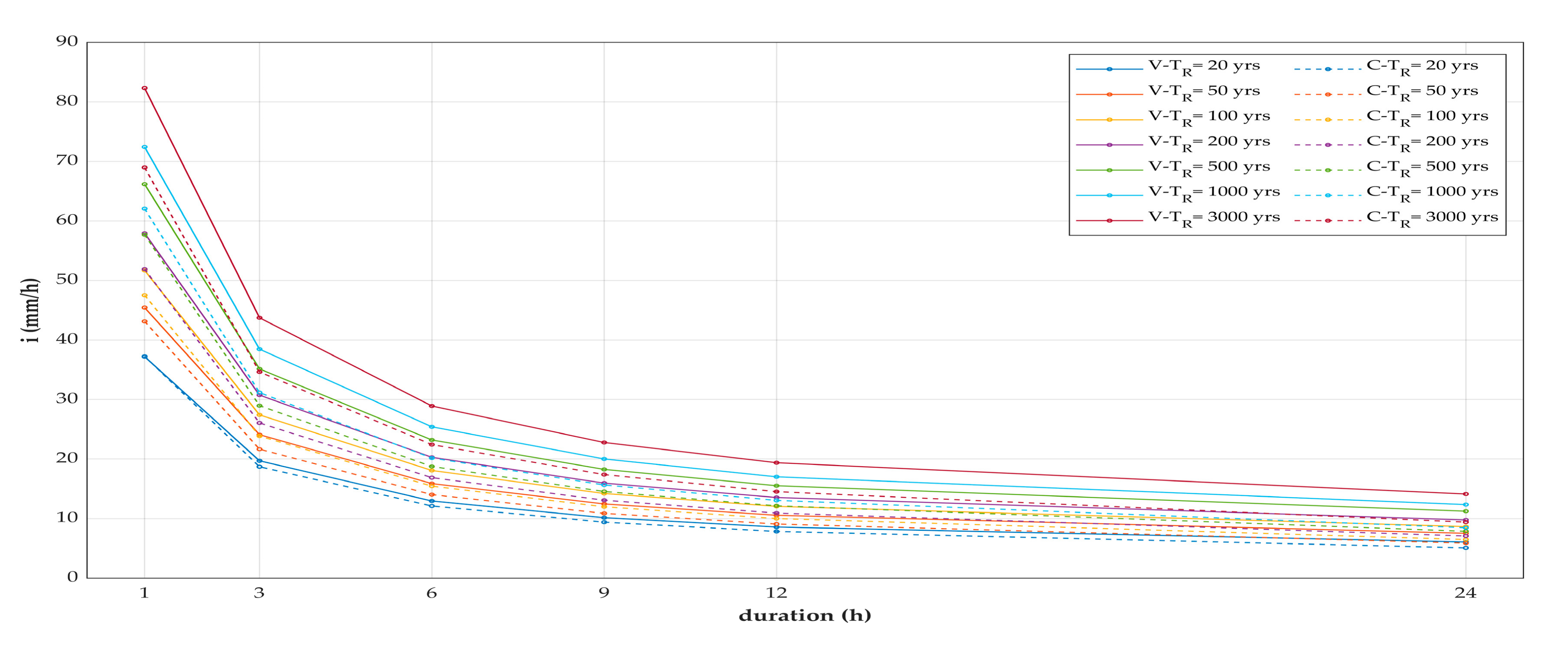
The intensity–duration–area–frequency (IDAF) curves are derived for different return periods, both using CMORPH observations and VAPI regionalization procedure. In the former case, IDAFs were modelled with Gumbel probability distribution, which resulted to fit best the sample. In the latter approach, the areal reduction factor (ARF) has been applied to rainfall intensity to convert from punctual to areal precipitation. The IDAF curves derived for different return periods and with both methods are shown in Figure 3. The colour of the curves changes for each return period, while the line style varies with the data source, having the continuous line for the curves built with VAPI procedure and the dashed line for satellite-based IDAFs. Moreover, IDAFs related to VAPI regionalization approach are marked with letter V in the legend, while CMORPH-based curves are identified with letter C. The analysis of IDAFs revealed that, for each return period $T_R$, CMORPH-based IDAFs provide lower values of precipitation intensity, with the only exception of $T_R$ = 20 years and duration $d$ = 1 h. This general tendency to underestimate rainfall intensity, however, varies with the return period: for low return periods, IDAF curves built with the two approaches are almost overlapping, but the more the return period increases, the more the curves distance increases.

4.3. Peak Flow and Spillway Dimension

The flow peak discharges are computed by the mean of the rational formula (Equation (9)), for fixed durations and return periods. The rainfall intensity that appears in Equation (9) is derived from IDAF curves, built both with CMORPH observations and with the VAPI regionalization procedure. The design peak is found setting the duration of the rainfall event equal to the concentration time of the catchment, which resulted to be $t_c$ = 9 h, and for a 3000-year return period [44]. Nevertheless, as lower return periods are usually needed for the design of other components of the dam and for other kind of dams (e.g., concrete dams) [44], the peak discharges are computed also for the return periods of 20, 50, 100, 200, 500, and 1000 years.

The results are presented in

Table 6. Peak flow computed from CMORPH-based IDAF curves.

$\mathit{d}$ (hours)	$\mathit{Q}$ (m3/s)
	${\mathit{T}}_{\mathit{R}}\mathbf{=}\mathbf{20}$ (years)	${\mathit{T}}_{\mathit{R}}\mathbf{=}\mathbf{50}$ (years)	${\mathit{T}}_{\mathit{R}}\mathbf{=}\mathbf{100}$ (years)	${\mathit{T}}_{\mathit{R}}\mathbf{=}\mathbf{200}$ (years)	${\mathit{T}}_{\mathit{R}}=500$ (years)	${\mathit{T}}_{\mathit{R}}\mathbf{=}\mathbf{1000}$ (years)	${\mathit{T}}_{\mathit{R}}\mathbf{=}\mathbf{3000}$ (years)
1	1866.2	2160.2	2380.5	2600.0	2889.6	3108.5	3455.3
3	937.0	1084.6	1195.3	1305.5	1450.9	1560.8	1734.9
6	606.7	702.3	773.9	845.3	939.4	1010.6	1123.3
9	470.5	544.6	600.1	655.5	728.5	783.7	871.1
12	392.8	454.7	501.1	547.3	608.2	654.3	727.3
24	254.3	294.4	324.4	354.3	393.8	423.6	470.9

and

Table 7. Peak flow computed from VAPI-based IDAF curves.

$\mathit{d}$ (hours)	$\mathit{Q}$ (m3/s)
	${\mathit{T}}_{\mathit{R}}\mathbf{=}\mathbf{20}$ (years)	${\mathit{T}}_{\mathit{R}}\mathbf{=}\mathbf{50}$ (years)	${\mathit{T}}_{\mathit{R}}\mathbf{=}\mathbf{100}$ (years)	${\mathit{T}}_{\mathit{R}}\mathbf{=}\mathbf{200}$ (years)	${\mathit{T}}_{\mathit{R}}\mathbf{=}\mathbf{500}$ (years)	${\mathit{T}}_{\mathit{R}}\mathbf{=}\mathbf{1000}$ (years)	${\mathit{T}}_{\mathit{R}}\mathbf{=}\mathbf{3000}$ (years)
1	1862.9	2276.3	2589.0	2901.7	3315.1	3627.8	3940.5
3	986.8	1206.9	1373.4	1540.0	1760.1	1926.6	2093.1
6	649.1	795.2	905.7	1016.2	1162.4	1272.9	1383.4
9	508.4	624.1	711.6	799.1	914.8	1002.3	1089.9
12	429.7	528.7	603.5	678.4	777.4	852.2	927.1
24	303.4	377.2	433.1	489.0	562.8	618.7	674.5

, respectively. The flow peaks values obtained confirmed that, in general, using satellite-based IDAF curves leads to an underestimation with respect to the regionalization approach. The only exception is represented by the 20-years return period and 1-h duration event, for which CMORPH-based rainfall intensity overestimates the flow peak.

These outcomes are more evident observing

Table 8. Mean Bias Error between peak discharges estimated with CMORPH data and VAPI project.

$\mathit{d}$ (hours)	$\mathit{M}\mathit{B}{\mathit{E}}_{\mathit{Q}}$ (%)
	${\mathit{T}}_{\mathit{R}}\mathbf{=}\mathbf{20}$ (years)	${\mathit{T}}_{\mathit{R}}\mathbf{=}\mathbf{50}$ (years)	${\mathit{T}}_{\mathit{R}}\mathbf{=}\mathbf{100}$ (years)	${\mathit{T}}_{\mathit{R}}\mathbf{=}\mathbf{200}$ (years)	${\mathit{T}}_{\mathit{R}}\mathbf{=}\mathbf{500}$ (years)	${\mathit{T}}_{\mathit{R}}\mathbf{=}\mathbf{1000}$ (years)	${\mathit{T}}_{\mathit{R}}\mathbf{=}\mathbf{3000}$ (years)
1	0.2	−5.1	−8.1	−10.4	−12.8	−14.3	−15.6
3	−5.0	−10.1	−13.0	−15.2	−17.6	−19.0	−20.2
6	−6.5	−11.7	−14.6	−16.8	−19.2	−20.6	−21.8
9	−7.5	−12.7	−15.7	−18.0	−20.4	−21.8	−23.0
12	−8.6	−14.0	−17.0	−19.3	−21.8	−23.2	−24.5
24	−16.2	−22.0	−25.1	−27.5	−30.0	−31.5	−32.8

, where the mean bias error ($MB{E}_Q$) is computed for each flow peak referred to a specific duration and return period. MBE is computed considering the discharges derived with the regionalization approach as the benchmark. Looking at Table 8 it can be noticed that, for a fixed $T_R$, the $MB{E}_Q$ associated to the peak discharge increases (in absolute terms) when rainfall duration grows. On the other hand, for the same duration $d$, the error increases for higher return periods. The lowest (absolute) error is obtained for 20-years return period and one-hour duration rainfall event ($MB{E}_Q$= 0.18). Unsurprisingly, the highest bias is found for 3000-years return period and 24-h duration event.

The spillway length is computed using Equation (12) and adopting the 3000-years return period flow peak as the design discharge. It is therefore evaluated employing both the CMORPH and the VAPI-based discharges. The maximum head over the weir crest $H$ is set equal to 2.65 m and the flow coefficient $\mu$ for the maximum head is 0.485. The resulting length of the spillway, as expected, is higher when using the design peak given by the regionalization approach, since the design discharge is greater for VAPI than for satellite-based IDAFs. The corresponding lengths of the spillway are $L_C$ = 94 m for the satellite-based design discharge and $L_V$ = 124 m for the VAPI-based design peak, with a difference of 30 m between the two approaches.

5. Discussion

CMORPH performances across the globe have been extensively studied in the past years, with different technique, i.e., point–pixel [33,35], pixel–pixel [22,23], using different statistics and different spatial and temporal resolution of the data set. The results found are thus site specific, nevertheless some major conclusions can be drawn. As CMORPH is based on passive microwave (PMW) satellite information, its estimates are influenced by topography, climatology, complexity of the terrain e proximity to water bodies, as enlighted, for instance, by Tian and Peters-Lidard [68], Kidd [69] and Stampoulis [67]. Moreover, CMORPH was found to perform better during warm seasons rather than in cold ones, with an underestimation of precipitation [68,69], as PMW estimates suffer for snow and ice contaminations [67,68]. This tendency was confirmed in different parts of the globe, such as in the South-East of United States of America, where CMORPH had higher probability of detection (POD) values, higher correlation and poorer root squared mean error (RMSE) [70], over the Amazon basin, where it better detects rainfall in summer [71], and over continental Europe [67]. The satellite data set was also found to perform differently according to rainfall intensity, with increasing underestimation for higher rainfall intensity [12,67]. To this regard, Marra et al. [12], when analysing CMORPH skills in deriving IDF curves, found that satellite performance varies with climate: for an area with Mediterranean climate, satellite underestimates rain rate at different durations; where the climate is arid, CMORPH tends to overestimate precipitation at the low return periods and tend to converge to the rain gauge estimate when return period increases; for a basin with semi-arid climate, however, satellite underestimates rainfall rain rate for low return periods and tend to converge to the rain gauge-based intensity when return period increases.

Due to the high variability of CMORPH performance with terrain complexity, proximity to water bodies and climate, a quantitative comparison of the evaluation indexes computed in this work and the same metrics found in other works, with different case studies, cannot be made. To the authors’ knowledge, there are two works which involved the evaluation of CMORPH performance in Sicily, one carried out by Lo Conti [22] et al. and the other by Stampoulis [67]. In the former, the authors compute several evaluation metrics varying the temporal aggregation of the satellite data set, adopting the pixel–pixel comparison method. Their results show that all the indexes improve with increasing aggregation time and CMORPH performed best in the central part of Sicily, in terms of correlation coefficient (CC), as it is the furthest area from the Mediterranean Sea. For the daily scale, the authors provide average values over Sicily for the evaluation indexes. The values they obtained, i.e., POD and FAR around 0.45, CC slightly below 0.6, confirmed our results.

In the latter study, Stampoulis et al. [67] employed daily satellite observations and evaluated them against rain gauge data. It resulted that both for the warm and the cold season, the correlation coefficient of the central-eastern part of the island is around 0.6, confirming, also in this case, our findings.

The rainfall intensity values provided by the satellite-based intensity–duration–area–frequency curves differ from the corresponding values given by the VAPI project (Figure 3). The differences between the two curves, for the same duration, grow with increasing return period and, for same return period, grow with increasing duration of the rainfall event. One of the factors responsible for the differences with increasing return period is the different length of time series employed to build IDAF curves, as already found also by Marra et al. [12]. The statistical analysis of the VAPI project was conducted with the regionalization procedure, which ensures a robust estimation for high return periods. Conversely, CMORPH provides time series with 22 years of data due to the fact that this rainfall product is available only starting from 1998. Therefore, it is clear that the higher is the return period of the estimation, the more the estimation is affected by uncertainties and results should be handled with caution.

When comparing the IDAF curves obtained with the two methods (Figure 3), it should also be noted that they are obtained employing two different probability distributions, which could cause differences in the rainfall intensity values obtained.

Despite the uncertainties related to the high return periods estimates, the satellite-based IDAF curves provide similar results to the VAPI-based curves at the low return periods, especially for short duration events. CMORPH could be, therefore, successfully employed for the design of low return period structures in ungauged catchments. On the other hand, for the design of hydraulic structures with high return period, as in this case for the spillway of a dam, caution is needed when satellite observations are employed for the statistical analysis of hydrological data. For the case study, for instance, the error in the peak discharge computation is −23.7% for 3000 years of return period, which determines a considerable variation, i.e., 30 m, in the design length of the spillway.

CMORPH observations could be employed to identify the design storm and, thus, the design flow peak together with a corrective coefficient, which operates to adjust the estimated flow peak value. As this method should be used in ungauged areas, it should be possible to compute the corrective coefficients without the comparison between regionalization studies and satellite observations. This study represents a pivotal work, future research should investigate more case studies, with different topography and climate to establish, if possible, a general relationship or a range of variation for the corrective coefficient, which allows for the correct evaluation of the design discharge. Moreover, satellite data will increase their length over time as their main limit is their availability from 1998 only. Over time a more robust time series will be available and a more comprehensive comparison with precipitation from rain gauges will be possible.

6. Conclusions

Satellite precipitation products could be an alternative valuable source of hydrological data to design hydraulic structures in remote and ungauged areas. In this paper, we use CMORPH rainfall estimates to derive design peak flows for different return periods and we compare them with the corresponding quantities computed from the VAPI regionalization project, used in ungauged areas in Italy. The design peak flows are computed throughout the rational method: the design storm is identified throughout the intensity–duration–area–frequency (IDAF) curves, built for both satellite observations and applying the VAPI method. To assess weakness and potential of the satellite products, the design flow is estimated from the design storm. Then, to quantify the effects of the use of satellite data for design purposes, we provide an applicative example for the calculation of the design length of a spillway of a dam. The study is applied to the Pietrarossa catchment, in southern Italy, where a rockfill dam is located and a regionalization study, i.e., VAPI, is available. A prior evaluation of CMORPH estimates performance against the rain gauge observations for the case study is also conducted, using both categorical and continuous statistical metrics. Our findings showed that the satellite data set correlates poorly with rain gauges for the 30-min temporal scale, but its performance increase with increasing temporal aggregation, reaching an average correlation coefficient of 0.65. The skills in detecting rainfall also improve, reaching an average probability of detection equal to 0.43. Our findings are in line with previous studies conducted in Sicily.

Results also revealed that CMORPH observations tend to underestimate precipitation intensity for each duration and each return period, with the exception of the 1-h duration and 20-years return period rainfall event, for which using satellite data slightly overestimates rainfall intensity. The storm design underestimation in turns implies the underestimation of design peak flows, which increases with growing of return period and event duration. The main factors responsible for these differences are to be found in the different length of hydrological time series employed and in the different probability distribution adopted to describe rainfall intensities. We therefore suggest to use with caution rainfall from satellite to design hydraulic structures as the uncertainty is high especially for high return periods. For instance, in the applicative example provided, using satellite-based design storm led to an underestimation of the design peak discharge that increases with return period, ranging from 7.5% for 20-years return period to 23% for 3000-years return period. The underestimation of the design discharge in turns determines the underestimation of the spillway length equal to 30 m, which cannot be neglected.

Despite the uncertainties in the estimation of design storms at high return periods, CMORPH performed well at low return periods and durations. It could be thus adopted for hydraulic structures characterized by low return period.

The caveats of this work are to be found in the limited length of satellite records, as they are available only from 1998. As CMORPH performance varies with terrain complexity, proximity to water bodies and climate, the site choice can affect results. To untangle the latter limit, future studies could be aimed at investigating several catchments, with different climate and topography. A further development could be the definition of mathematical relationships or range values for a corrective coefficient to be applied to the CMORPH estimates, in order to be able to successfully employ the satellite data sets for the design of high return period structures in ungauged areas.

References

- Biscarini, C.; Di Francesco, S.; Ridolfi, E.; Manciola, P. On the simulation of floods in a narrow bending valley: The malpasset dam break case study. Water 2016, 8, 545. [Google Scholar] [CrossRef] [Green Version]
- ICOLD-International Commission On Large Dams. Dam Failures Statistical Analysis; ICOLD: Paris, France, 1995. [Google Scholar]
- Amarnath, C.R.; Thatikonda, S. Study on backwater effect due to Polavaram Dam Project under different return periods. Water 2020, 12, 576. [Google Scholar] [CrossRef] [Green Version]
- De Michele, C.; Salvadori, G.; Canossi, M.; Petaccia, A.; Rosso, R. Bivariate statistical approach to check adequacy of dam spillway. J. Hydrol. Eng. 2005, 10. [Google Scholar] [CrossRef]
- Domínguez, M.R.; Arganis, J.M.L. Validation of methods to estimate design discharge flow rates for dam spillways with large regulating capacity. Hydrol. Sci. J. 2012, 57. [Google Scholar] [CrossRef] [Green Version]
- Reed, D.; Stewart, E. Dam safety: An evaluation of some procedures for design flood estimation. Hydrol. Sci. J. 1991, 36, 487–490. [Google Scholar] [CrossRef]
- Sordo-Ward, A.; Garrote, L.; Martín-Carrasco, F.; Dolores Bejarano, M. Extreme flood abatement in large dams with fixed-crest spillways. J. Hydrol. 2012, 466–467. [Google Scholar] [CrossRef] [Green Version]
- Grimaldi, S.; Petroselli, A.; Serinaldi, F. Design hydrograph estimation in small and ungauged watersheds: Continuous simulation method versus event-based approach. Hydrol. Process. 2012, 26. [Google Scholar] [CrossRef]
- Cameron, D.; Beven, K.; Naden, P. Flood frequency estimation by continuous simulation under climate change (with uncertainty). Hydrol. Earth Syst. Sci. 2000, 4. [Google Scholar] [CrossRef]
- Blazkova, S.; Beven, K. Flood frequency estimation by continuous simulation of subcatchment rainfalls and discharges with the aim of improving dam safety assessment in a large basin in the Czech Republic. J. Hydrol. 2004, 292. [Google Scholar] [CrossRef]
- Efstratiadis, A.; Koussis, A.D.; Koutsoyiannis, D.; Mamassis, N. Flood design recipes vs. reality: Can predictions for ungauged basins be trusted? Nat. Hazards Earth Syst. Sci. 2014, 14. [Google Scholar] [CrossRef] [Green Version]
- Marra, F.; Morin, E.; Peleg, N.; Mei, Y.; Anagnostou, E.N. Intensity-duration-frequency curves from remote sensing rainfall estimates: Comparing satellite and weather radar over the eastern Mediterranean. Hydrol. Earth Syst. Sci. 2017, 21. [Google Scholar] [CrossRef] [Green Version]
- Walker, D.; Forsythe, N.; Parkin, G.; Gowing, J. Filling the observational void: Scientific value and quantitative validation of hydrometeorological data from a community-based monitoring programme. J. Hydrol. 2016, 538, 713–725. [Google Scholar] [CrossRef] [Green Version]
- Dai, Q.; Bray, M.; Zhuo, L.; Islam, T.; Han, D. A Scheme for Rain Gauge Network Design Based on Remotely Sensed Rainfall Measurements. J. Hydrometeorol. 2017, 18, 363–379. [Google Scholar] [CrossRef]
- Narbondo, S.; Gorgoglione, A.; Crisci, M.; Chreties, C. Enhancing physical similarity approach to predict runoff in ungauged watersheds in sub-tropical regions. Water 2020, 12, 528. [Google Scholar] [CrossRef] [Green Version]
- Joyce, R.J.; Janowiak, J.E.; Arkin, P.A.; Xie, P. CMORPH: A method that produces global precipitation estimates from passive microwave and infrared data at high spatial and temporal resolution. J. Hydrometeorol. 2004. [Google Scholar] [CrossRef]
- Hsu, K.L.; Gao, X.; Sorooshian, S.; Gupta, H.V. Precipitation estimation from remotely sensed information using artificial neural networks. J. Appl. Meteorol. 1997, 36, 1176–1190. [Google Scholar] [CrossRef]
- Huffman, G.J.; Adler, R.F.; Bolvin, D.T.; Gu, G.; Nelkin, E.J.; Bowman, K.P.; Hong, Y.; Stocker, E.F.; Wolff, D.B. The TRMM Multisatellite Precipitation Analysis (TMPA): Quasi-global, multiyear, combined-sensor precipitation estimates at fine scales. J. Hydrometeorol. 2007, 8, 38–55. [Google Scholar] [CrossRef]
- Funk, C.; Peterson, P.; Landsfeld, M.; Pedreros, D.; Verdin, J.; Shukla, S.; Husak, G.; Rowland, J.; Harrison, L.; Hoell, A.; et al. The climate hazards infrared precipitation with stations—A new environmental record for monitoring extremes. Sci. Data 2015, 2. [Google Scholar] [CrossRef] [Green Version]
- Stampoulis, D.; Anagnostou, E.N.; Nikolopoulos, E.I. Assessment of high-resolution satellite-based rainfall estimates over the mediterranean during heavy precipitation events. J. Hydrometeorol. 2013, 14. [Google Scholar] [CrossRef]
- Mazzoleni, M.; Brandimarte, L.; Amaranto, A. Evaluating precipitation datasets for large-scale distributed hydrological modelling. J. Hydrol. 2019. [Google Scholar] [CrossRef] [Green Version]
- Lo Conti, F.; Hsu, K.L.; Noto, L.V.; Sorooshian, S. Evaluation and comparison of satellite precipitation estimates with reference to a local area in the Mediterranean Sea. Atmos. Res. 2014. [Google Scholar] [CrossRef] [Green Version]
- Duan, Z.; Liu, J.; Tuo, Y.; Chiogna, G.; Disse, M. Evaluation of eight high spatial resolution gridded precipitation products in Adige Basin (Italy) at multiple temporal and spatial scales. Sci. Total Environ. 2016. [Google Scholar] [CrossRef] [PubMed] [Green Version]
- Ombadi, M.; Nguyen, P.; Sorooshian, S.; Hsu, K.L. Developing Intensity-Duration-Frequency (IDF) Curves From Satellite-Based Precipitation: Methodology and Evaluation. Water Resour. Res. 2018, 54. [Google Scholar] [CrossRef]
- Cannarozzo, M.; D’Asaro, F.; Ferro, V. Regional rainfall and flood frequency analysis for Sicily using the two component extreme value distribution. Hydrol. Sci. J. 1995, 40. [Google Scholar] [CrossRef] [Green Version]
- Berga, L.; Buil, J.M.; Bofill, E.; Cea, J.C.D.; Perez, J.A.G.; Mañueco, G.; Polimon, J.; Soriano, A.; Yagüe, J. (Eds.) Dams and Reservoirs, Societies and Environment in the 21st Century, Two Volume Set; CRC Press: Boca Raton, FL, USA, 2006. [Google Scholar]
- Xie, P.; Joyce, R.; Wu, S.; Yoo, S.H.; Yarosh, Y.; Sun, F.; Lin, R. Reprocessed, bias-corrected CMORPH global high-resolution precipitation estimates from 1998. J. Hydrometeorol. 2017. [Google Scholar] [CrossRef]
- Xie, P.; Xiong, A.Y. A conceptual model for constructing high-resolution gauge-satellite merged precipitation analyses. J. Geophys. Res. Atmos. 2011. [Google Scholar] [CrossRef]
- Sapiano, M.R.P.; Arkin, P.A. An intercomparison and validation of high-resolution satellite precipitation estimates with 3-hourly gauge data. J. Hydrometeorol. 2009, 10, 149–166. [Google Scholar] [CrossRef]
- Requena, A.I.; Mediero, L.; Garrote, L. A bivariate return period based on copulas for hydrologic dam design: Accounting for reservoir routing in risk estimation. Hydrol. Earth Syst. Sci. 2013, 17, 3023–3038. [Google Scholar] [CrossRef] [Green Version]
- Ferrari, E.; Versace, P. La Valutazione Delle Piene in Italia; Gruppo Nazionale per la Difesa dalle Catastrofi Idrogeologiche; Consiglio Nazionale delle Ricerche: Rome, Italy, 1994. [Google Scholar]
- Bhatti, H.A.; Rientjes, T.; Haile, A.T.; Habib, E.; Verhoef, W. Evaluation of bias correction method for satellite-based rainfall data. Sensors 2016, 16, 884. [Google Scholar] [CrossRef] [Green Version]
- Gumindoga, W.; Rientjes, T.H.M.; Haile, A.T.; Makurira, H.; Reggiani, P. Performance evaluation of CMORPH satellite precipitation product in the Zambezi Basin. Int. J. Remote Sens. 2019, 40. [Google Scholar] [CrossRef]
- Gumindoga, W.; Rientjes, T.H.M.; Haile, A.T.; Makurira, H.; Reggiani, P. Performance of bias-correction schemes for CMORPH rainfall estimates in the Zambezi River basin. Hydrol. Earth Syst. Sci. 2019, 23. [Google Scholar] [CrossRef] [Green Version]
- Zhang, C.; Chen, X.; Shao, H.; Chen, S.; Liu, T.; Chen, C.; Ding, Q.; Du, H. Evaluation and intercomparison of high-resolution satellite precipitation estimates-GPM, TRMM, and CMORPH in the Tianshan Mountain Area. Remote Sens. 2018, 10, 543. [Google Scholar] [CrossRef] [Green Version]
- Hughes, D.A. Comparison of satellite rainfall data with observations from gauging station networks. J. Hydrol. 2006, 327. [Google Scholar] [CrossRef]
- Lopez, V.; Napolitano, F.; Russo, F. Calibration of a rainfall-runoff model using radar and raingauge data. Adv. Geosci. 2005, 2. [Google Scholar] [CrossRef] [Green Version]
- Russo, F.; Napolitano, F.; Gorgucci, E. Rainfall monitoring systems over an urban area: The city of Rome. Hydrol. Process. 2005, 19, 1007–1019. [Google Scholar] [CrossRef]
- Panthou, G.; Vischel, T.; Lebel, T.; Quantin, G.; Molinié, G. Characterizing the space–time structure of rainfall in the Sahel with a view to estimating IDAF curves. Hydrol. Earth Syst. Sci. Discuss. 2014, 11. [Google Scholar] [CrossRef]
- Caporali, E.; Cavigli, E.; Petrucci, A. The index rainfall in the regional frequency analysis of extreme events in Tuscany (Italy). Environmetrics 2008, 19. [Google Scholar] [CrossRef]
- Forestieri, A.; Lo Conti, F.; Blenkinsop, S.; Cannarozzo, M.; Fowler, H.J.; Noto, L.V. Regional frequency analysis of extreme rainfall in Sicily (Italy). Int. J. Climatol. 2018, 38. [Google Scholar] [CrossRef]
- Ferro, V.; Porto, P. Regional analysis of rainfall-depth-duration equation for South Italy. J. Hydrol. Eng. 1999. [Google Scholar] [CrossRef]
- Bonaccorso, B.; Aronica, G.T. Estimating Temporal Changes in Extreme Rainfall in Sicily Region (Italy). Water Resour. Manag. 2016, 30. [Google Scholar] [CrossRef]
- Ministero delle Infrastrutture e dei Trasporti. Norme Tecniche per la Progettazione e la Costruzione Degli Sbarramenti di Ritenuta (Dighe e Traverse); Ministero delle Infrastrutture e dei Trasporti: Rome, Italy, 2014. [Google Scholar]
- Langousis, A.; Kaleris, V. Theoretical framework to estimate spatial rainfall averages conditional on river discharges and point rainfall measurements from a single location: An application to western Greece. Hydrol. Earth Syst. Sci. 2013, 17. [Google Scholar] [CrossRef] [Green Version]
- Mineo, C.; Ridolfi, E.; Napolitano, F.; Russo, F. The areal reduction factor: A new analytical expression for the Lazio Region in central Italy. J. Hydrol. 2018, 560. [Google Scholar] [CrossRef]
- Mineo, C.; Ridolfi, E.; Neri, A.; Russo, F. Areal reduction factor: The effect of the return period. AIP Conf. Proc. 2019, 2116. [Google Scholar] [CrossRef] [Green Version]
- Svensson, C.; Jones, D.A. Review of methods for deriving areal reduction factors. J. Flood Risk Manag. 2010, 3. [Google Scholar] [CrossRef] [Green Version]
- Koutsoyiannis, D.; Xanthopoulos, T. Hydrology Engineering, 3rd ed.; Technical University of Athens: Athens, Greece, 1999. [Google Scholar]
- Thiessen, A.H. Precipitation averages for large areas. Mon. Weather Rev. 1911, 7, 1082–1089. [Google Scholar] [CrossRef]
- Chow, V.T.; Maidment, D.R.; Mays, L.W. Applied Hydrology; McGraw-Hill Book Company: New York, NY, USA, 1988. [Google Scholar]
- De Luca, D.L.; Galasso, L. Stationary and non-stationary frameworks for extreme rainfall time series in southern Italy. Water 2018, 10, 477. [Google Scholar] [CrossRef] [Green Version]
- Koutsoyiannis, D.; Kozonis, D.; Manetas, A. A mathematical framework for studying rainfall intensity-duration-frequency relationships. J. Hydrol. 1998, 206. [Google Scholar] [CrossRef]
- Shrestha, A.; Babel, M.S.; Weesakul, S.; Vojinovic, Z. Developing Intensity-Duration-Frequency (IDF) curves under climate change uncertainty: The case of Bangkok, Thailand. Water 2017, 9, 145. [Google Scholar] [CrossRef] [Green Version]
- Papalexiou, S.M.; Koutsoyiannis, D.; Makropoulos, C. How extreme is extreme? An assessment of daily rainfall distribution tails. Hydrol. Earth Syst. Sci. 2013, 17. [Google Scholar] [CrossRef] [Green Version]
- Marra, F.; Nikolopoulos, E.I.; Anagnostou, E.N.; Bárdossy, A.; Morin, E. Precipitation frequency analysis from remotely sensed datasets: A focused review. J. Hydrol. 2019, 574. [Google Scholar] [CrossRef]
- Bernard, M.M. Formulas for Rainfall Intensities of Long Duration. Trans. Am. Soc. Civ. Eng. 1932, 96, 592–606. [Google Scholar]
- Pagliara, S.; Viti, C. Discussion of “Rainfall Intensity-Duration-Frequency Formula for India” by Umesh C. Kothyari and Ramachandra J. Garde (February, 1992, Vol. 118, No. 2). J. Hydraul. Eng. 1993, 119. [Google Scholar] [CrossRef]
- Asare-Kyei, D.; Forkuor, G.; Venus, V. Modeling flood hazard zones at the sub-district level with the rational model integrated with GIS and remote sensing approaches. Water 2015, 7, 3531–3564. [Google Scholar] [CrossRef] [Green Version]
- McCuen, R.H. Uncertainty analyses of watershed time parameters. J. Hydrol. Eng. 2009, 14. [Google Scholar] [CrossRef]
- Giandotti, M. Previsione delle piene e delle magre dei corsi d’acqua. Ist. Poligr. Stato 1934, 8, 107–117. [Google Scholar]
- Kirpich, Z.P. Time of concentration of small agricultural watersheds. Civ. Eng. 1940, 10, 362. [Google Scholar]
- NRCS (National Research Conservation Service). Ponds—Planning, Design, Construction; NRCS: Washington, DC, USA, 1997. [Google Scholar]
- Young, C.B.; McEnroe, B.M.; Rome, A.C. Empirical Determination of Rational Method Runoff Coefficients. J. Hydrol. Eng. 2009, 14. [Google Scholar] [CrossRef]
- Grimaldi, S.; Petroselli, A. Do we still need the Rational Formula? An alternative empirical procedure for peak discharge estimation in small and ungauged basins. Hydrol. Sci. J. 2015, 60. [Google Scholar] [CrossRef]
- De Benedetti, S. Diga in Materiali Sciolti Sul Fiume Margherito. Master’s Thesis, La Sapienza Università di Roma, Roma, Italy, 1985. [Google Scholar]
- Stampoulis, D.; Anagnostou, E. Evaluation of global satellite rainfall products over Continental Europe. J. Hydrometeorol. 2012, 13. [Google Scholar] [CrossRef]
- Tian, Y.; Peters-Lidard, C.D. A global map of uncertainties in satellite-based precipitation measurements. Geophys. Res. Lett. 2010, 37. [Google Scholar] [CrossRef]
- Kidd, C.; Bauer, P.; Turk, J.; Huffman, G.J.; Joyce, R.; Hsu, K.L.; Braithwaite, D. Intercomparison of high-resolution precipitation products over Northwest Europe. J. Hydrometeorol. 2012, 13. [Google Scholar] [CrossRef] [Green Version]
- Tian, Y.; Peters-Lidard, C.D.; Choudhury, B.J.; Garcia, M. Multitemporal analysis of TRMM-based satellite precipitation products for land data assimilation applications. J. Hydrometeorol. 2007, 8. [Google Scholar] [CrossRef]
- Pereira Filho, A.J.; Carbone, R.E.; Janowiak, J.E.; Arkin, P.; Joyce, R.; Hallak, R.; Ramos, C.G.M. Satellite rainfall estimates over South America—Possible applicability to the water management of large watersheds. J. Am. Water Resour. Assoc. 2010, 46. [Google Scholar] [CrossRef]
Figure 1.
Case study: (a) catchment location (red) in Italy; (b) Pietrarossa catchment map.
Figure 2.
Scatter plots of 30-min and daily observations of rain gauges and CMORPH. The blue points stand for the daily observations, the black line represents the bisect, the red continuous line stands for the interpolant of the daily observations and the red dashed line is the interpolant of the 30-min observations. Each scatter plot is referred to a station: (a) Aidone; (b) Caltagirone; (c) Caltanissetta; (d) Enna; (e) Gela; (f) Mazzarino; (g) Mazzarrone; (h) Mineo; (i) Piazza Armerina; (l) Riesi.