Interaction among Controlling Factors on Riverine DIN Export in Small Mountainous Rivers of Taiwan: Inseparable Human-Landscape System

Abstract

Increasing anthropogenic nitrogen (N) emission via different pathways has shown prominent impact on aquatic ecosystems for decades, but the effects of interaction among climate-, landscape- and human-associated variables on riverine DIN (dissolved inorganic nitrogen, mainly NO₃⁻ and NH₄⁺) export are unclear. In this study, the data of 43 watersheds with a wide range of climate-, landscape- and human-associated gradients across Taiwan were evaluated with partial redundancy analysis (pRDA) to examine their interactive controls on riverine DIN export. Results show that the annual riverine DIN export in Taiwan is approximately 3100 kg-N km⁻² yr⁻¹, spanning from 230 kg-N km⁻² yr⁻¹ in less disturbed watersheds (eastern and central Taiwan) to 10,000 kg-N km⁻² yr⁻¹ in watersheds with intensive human intervention (southwestern and northern Taiwan). NO₃⁻ is generally the single dominant form of DIN, while NH₄⁺ renders significance in disturbed watersheds. Nearly all environmental variables display a positive correlation with DIN export, except for landscape setting variables (e.g., slope, area, channel length), which show a negative relationship. In terms of seasonal pattern, climate and human-landscape variables are related to NO₃⁻ export independently in the wet season, yet in the dry season climate-human variables jointly dominate NO₃⁻ export. Meanwhile, human-landscape (LH) variables (λ₁ of LH > 0.60) control NH₄⁺ exports in both seasons, and human-associated (H) variables (λ₁ of H = 0.13) have a minor effect on NH₄⁺ exports in dry season. Precisely, the contribution of controlling variables on DIN export vary with species and seasons, indicating water quality management could be time-dependent, which should be taken into consideration for designing mitigation strategies.

1. Introduction

Reactive nitrogen, a vital and essential nutrient for organisms and ecosystems, plays a key role in maintaining biodiversity and functions of ecosystems [1,2]. Over the past half century, the rapid increasing anthropogenic N emissions inevitably accelerated N deposition into the biosphere [3], and consequently exceeded the N-requirement for terrestrial ecosystems [4]. Studies show that N emissions and depositions have been declining in Europe and the U.S. since 2000, East and South Asia, in contrast, have become the hot spots of pollutant emissions due to population growth and intense agricultural activities [5,6]. Regions located near the emission source of East Asia receive excessive N deposition under favorable climatic conditions, such as the East Asian monsoon that blows directly to Taiwan with abundant rainfall [7]. The overloaded dissolved inorganic nitrogen (DIN) (majorly NO₃⁻, and NH₄⁺) led to eutrophication and harmful algal blooms which deteriorated water quality and caused damages in aquatic communities [8]. However, the DIN exports, particularly for seasonal changes, in subtropical mountainous watersheds are still unclear.

Many studies have demonstrated that even a mild replacement of natural vegetation with agricultural land use within watersheds would have significant impacts on hydrochemical processes [9,10], especially for DIN export from non-point pollution sources [11,12,13]. Landscape features such as slope, soil type/moisture, channel length, watershed area and relief may also regulate water quality [14]. In addition, climatic factors play a principal role in nutrient cycling in the era of warming climate and increasing extreme events. A warmer temperature will accelerate biogeochemical processes that would alter enzyme reactions, e.g., nitrification and denitrification, via microbial activities [15]. The torrential rainfall caused by synoptic weather, such as thunderstorms and tropical cyclones during summer, can bring approximately 30% to 50% of annual precipitation, such that a considerable amount of DIN will be flushed out, as evidenced in Taiwan [11,12]. However, the effects of the independent and interactive relationship among landscape patterns, climatic factors and anthropogenic disturbance are still not clear on riverine DIN export [16].

Previous analyses widely used linear or non-linear regression models to estimate the DIN export, but failed to separate the collinearity among variables, which might violate the statistical independent assumption [17]. To tackle the issues of collinearity, a series of well-developed methods, namely, principal components analysis (PCA), redundancy analysis (RDA) and partial RDA (pRDA), have been utilized to clarify the relative importance of independent variables and their interactive effects on dependent variables [18,19]. In this study, we apply PCA and pRDA to evaluate the contribution of climatic-, landscape- and human-associated variables and their interactions on DIN export based on 43 island-wide watersheds in Taiwan. This synthesis can help to disentangle the intertwined effects of these fundamental environmental factors on the behaviors of nutrient fluxes. Specifically, the objectives of this study are to (1) quantify riverine DIN export in subtropical watersheds in Taiwan, (2) explore the interplay of human disturbance, climatic factors and landscape characteristics on riverine NO₃⁻ and NH₄⁺ exports, respectively, and (3) figure out the spatial and seasonal variation of the controlling factors’ influences on DIN exports.

2. Materials and Methods

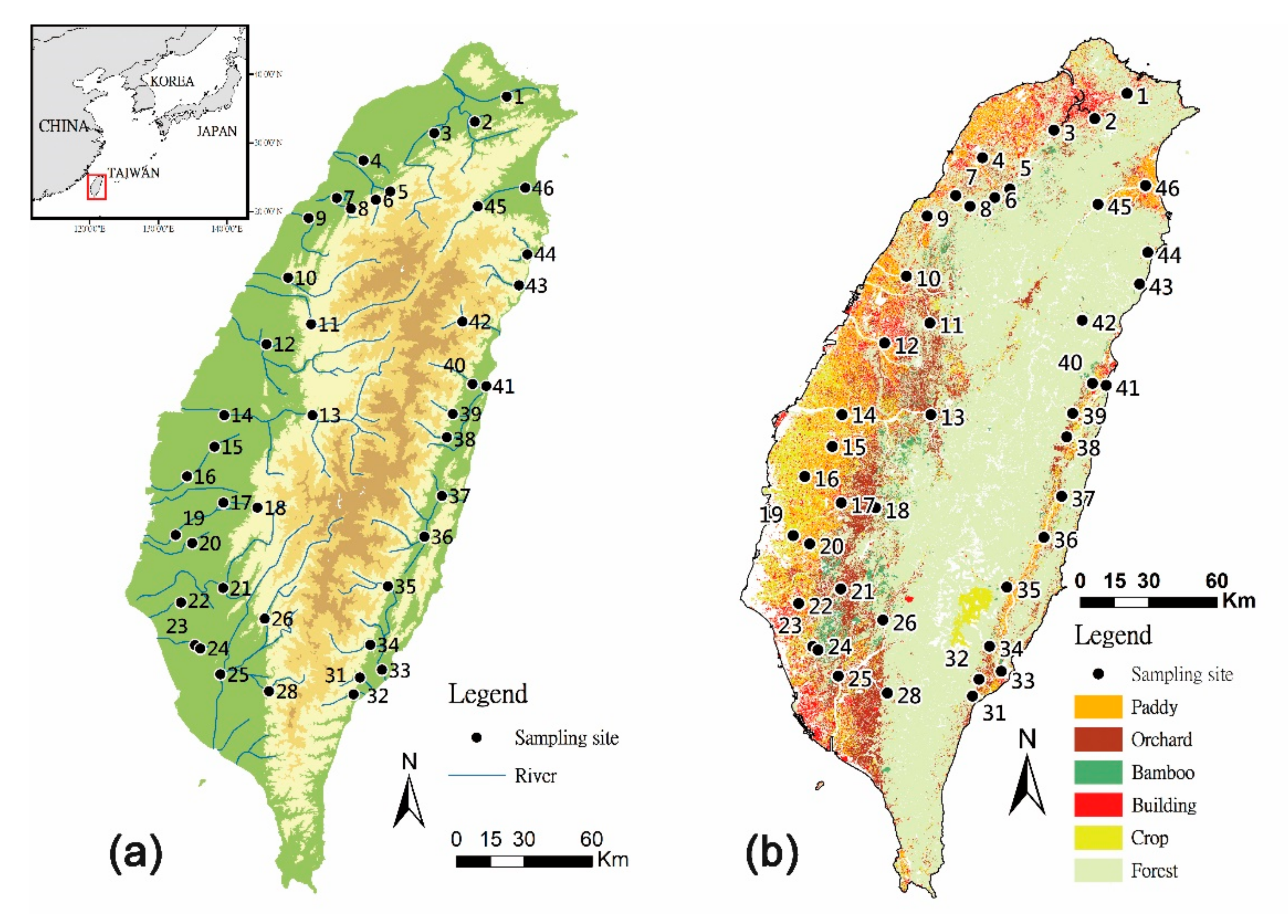
2.1. Study Site

Taiwan, located in the northwest Pacific Ocean, is a tropical/subtropical mountainous island in the East Asian monsoon climate zone. Elevation ranges from sea level to approximately 4000 m in a short horizontal distance (<75 km). The Tropic of Cancer crosses the central part of Taiwan, which divides the island into tropical monsoon climate in the south and subtropical monsoon climate in the north. The mean annual temperature (MAT) is 22 °C across the island, ranging from 15.0 °C/18.2 °C in the north/south in January to 28.7 °C/28.4 °C in July, and the MAT decreases with increasing altitude [20]. The mean annual precipitation (MAP) is 2500 mm for the entire island but shows high spatial variability ranging from less than 1500 mm in southwest Taiwan to over 4000 mm in the mountains of northeastern Taiwan [20]. There are more than 75% of MAP falls in the humid summer (May to October), while winter‒spring (November to April) is a relatively dry period.

Natural forests, plantation and bamboo forests cover 60% of the land, while farmlands and urbanized areas occupy 29% and 11%, respectively (Figure 1). The dominant vegetation types and land cover of Taiwan change from mixed and conifer forests at the mid and high elevation (>2000 m a.s.l.), evergreen broadleaf forests at the low and mid elevation (200−2000 m a.s.l.) to urban, buildup area and farmland on coastal plains (<800 m a.s.l.) (Figure 1). In this study, in order to estimate island-wide watershed DIN export, our sampling scheme covers a total of 43 sites. Individual watershed represented by each site can be as small as 82 km² and as large as 2969 km², and as a whole, they occupy more than 70% of the island and distribute evenly across Taiwan (Figure 1). Twenty-nine of the 43 watersheds are majorly covered by natural forest (>70% of forest cover), while 14 of the 43 are situated in the transition between mountain and plain regions where agricultural land cover and buildup area account for 10–65% and 0–18%, respectively (Figure 1 and Table S1). The average slope of the watersheds varies from 8% to 76%.

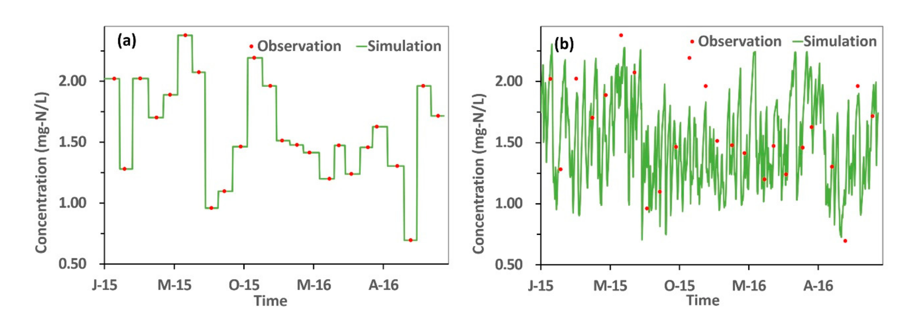
2.2. DIN Sampling and Streamflow Simulation

A monthly sampling scheme was conducted at all sampling sites (watersheds) during 2015–2016. Each route would be finished within 2 days. Stream water samples were collected by plunging a 1-L PE (polyethylene) bucket into stream, and the water was immediately filtered through 0.7 μm filters. A 15 mL subsample of filtrate was frozen on-site in liquid nitrogen and kept frozen until laboratory analysis at National Taiwan University. Nitrate, nitrite and ammonium content were analyzed using ion chromatography (IC) using a Dionex ICS−1500 (Thermo Fisher Scientific Inc.^® Sunnyvale, CA, USA) with a detection limit of 0.2, 0.2, and 0.4 μM, respectively. Our DIN calculation includes NO₂⁻, NO₃⁻ and NH₄⁺. Among them, nitrite is easily oxidized to nitrate and accounts for a small fraction (<5.0%). Therefore, we mainly analyzed and discussed NO₃⁻ and NH₄⁺.

Streamflow was acquired from the water level stations maintained by the Water Resource Agency (www.wra.gov.tw). The water level records were converted to streamflow via an individual rating curve and cross section approach. For some periods of missing records and ungauged sites, a hydrologic model (HBV, the Hydrologiska Byråns Vattenbalansavdelning model [21]) was used to fill the data gaps [22]. The historical observed daily streamflow was utilized to train the parameter set to fit low, normal and extreme values of simulated streamflow using the performance measure of NSE (Nash-Sutcliffe efficiency coefficient) [23]. The calibrated parameter set was then applied to the watersheds using their own climatic inputs and terrain information to simulate their daily streamflow during 2015–2016.

2.3. Export Estimation

Based on the discrete NO₃⁻ and NH₄⁺ concentration and continuous streamflow rates, individual NO₃⁻ and NH₄⁺ export of the 43 sites were then estimated using an R software package, loadflex, which provides several common methods (e.g., interpolations, regressions and composite method) for export estimation [24]. The composite method synthesizing rectangular interpolation and regression models is applied for export estimation. The mean values of two export methods in 2015 and 2016 were used as export results for further analysis. The rectangular interpolation has usually been used for studies on solute and sediment exports, where horizontal lines are drawn through observations in a plot of concentrations against time, and each horizontal line is connected to the next by a vertical line midway between successive observations [25]. The regression approach is a longstanding interpolation in estimating watershed solute exports (Figure 2). It often requires less data than other models if the data can span over the range of predictors instead of the full time period of interest [26]. A simple regression equation based on observed nutrient concentrations and concurrent streamflow (Q) with an exponent function is used to represent the hydrological influence on transport as Equation (1) below:

$$\mathrm{EXPORT}=\mathrm{m}{{\displaystyle \sum }}_{\mathrm{j}=1}^{\mathrm{T}}{\mathrm{Q}}_{\mathrm{j}}{\mathrm{C}}_{\mathrm{j}}=\mathrm{m}{{\displaystyle \sum }}_{\mathrm{j}=1}^{\mathrm{T}}{\mathrm{Q}}_{\mathrm{j}}{\mathrm{e}}^{{\mathrm{a}}_0+{\mathrm{a}}_1\ln \mathrm{Q}},$$

(1)

where Q_j [mm d⁻¹] is the daily streamflow rate on j-th day; C_j [mg-N L⁻¹] is an estimated concentration of NO₃⁻ and NH₄⁺ on the j-th day, m is the conversion factor to convert the calculated values into a specific unit [kg-N km⁻² yr⁻¹], and a₀ and a₁ are regressive coefficients. Coefficient a₀ is generally highly associated with the mean of observed nutrient concentration, and a₁ indicates the hydrological influence. A larger coefficient, a₁ (>0), indicates enhanced concentration with increasing streamflow, whereas a smaller value reflects the dilution effect because concentration decreases with the increase of discharge percentage. From Equation (1), we can estimate the concentration and export for non-measured days by introducing continuous daily streamflow [27]. According to the hydrologic seasonality, we summarized the daily export from May to October as wet season export and the summation of other daily exports as dry season export.

2.4. Variation Partitioning: PCA, RDA and pRDA

To tackle collinearity issues, many researchers have used principal components analysis (PCA) to reduce a number of correlated variables into a set of uncorrelated variables, which reserves its total variance and uncovers its hidden patterns [28]. In addition, in order to realize the relative importance of different explanatory variables and their interactive effects, direct gradient analysis such as redundancy analysis (RDA) and its successive partial constrained ordinations, i.e., partial RDA (pRDA) have been commonly proposed [18,19]. This allows researchers to explore the relationships between predictor variables and dependent variables by removing the intertwined effects among them [29]. However, most previous studies utilized PCA or RDA methods focusing on the relationship between biological phenomena and environmental influence, and there are only a few studies on water quality (e.g., [30]). Therefore, exploring the likely collinear controlling factors and their internal relationships to riverine DIN transport based on PCA and RDA will be valuable.

In order to interpret the spatial and temporal patterns of riverine NO₃⁻ and NH₄⁺ export and unravel the dependency among controlling factors, i.e., the human disturbance, climatic factors and landscape settings (

Table 1. Definition of different variables used in the three dimensions. Abbre. = abbreviation.

Dimension	Variables	Abbre.	Definition
Climatic Factors	Rainfall (mm)	RDry	Rainfall in dry season of the year
		RWet	Rainfall in wet season of the year
	Streamflow (mm)	SFDry	Discharge rate in dry season of the year
		SFWet	Discharge rate in wet season of the year
	Temperature (°C)	T	The degree of hotness or coldness of environment
Landscape Settings	Channel length (km)	CL	Total length of the stream channel
	Longest channel length (km)	LCL	The length of the longest stream channel in watershed
	Relief	Rel	The difference between the highest and lowest elevations in watershed
	Area (km2)	A	Drainage area of watershed
	Slope (%)	SLP100	The average slope in the 100 m buffer zone
		SLP200	The average slope in the 200 m buffer zone
		SLP500	The average slope in the 500 m buffer zone
		SLP1000	The average slope in the 1000 m buffer zone
		SLP2000	The average slope in the 2000 m buffer zone
		SLP	The average slope in watershed
	Drainage density(km−1)	DD	Total channel length over drainage area
	L/G (m)		The ratio of median flow path length to median flow path gradient
Human Disturbances	Population density (population km−2)	PD100	Population density in the 100 m buffer zone
		PD200	Population density in the 200 m buffer zone
		PD500	Population density in the 500 m buffer zone
		PD1000	Population density in the 1000 m buffer zone
		PD2000	Population density in the 2000 m buffer zone
		PD	Population density in watershed
	Buildup (%)	BD100	The percentage of buildup area in the 100 m buffer zone
		BD200	The percentage of buildup area in the 200 m buffer zone
		BD500	The percentage of buildup area in the 500 m buffer zone
		BD1000	The percentage of buildup area in the 1000 m buffer zone
		BD2000	The percentage of buildup area in the 2000 m buffer zone
		BD	The percentage of the buildup area in watershed
	Agriculture (%)	AGR100	The percentage of agriculture in the 100 m buffer zone
		AGR200	The percentage of agriculture in the 200 m buffer zone
		AGR500	The percentage of agriculture in the 500 m buffer zone
		AGR1000	The percentage of agriculture in the 1000 m buffer zone
		AGR2000	The percentage of agriculture in the 2000 m buffer zone
		AGR	The percentage of the agriculture in the watershed

), the whole analysis was carried out in three steps [29]: (i) the PCA was applied to find out a set of uncorrelated variables, (ii) detailed relations between export and each one of the controlling factors were displayed using a scatterplot matrix, and (iii) the RDA and pRDA were conducted to disentangle the contribution of the major variables.

PCA was applied to reduce redundant information and to transform the original correlated data into another set of uncorrelated variables. The PCA keeps only a few independent sets (patterns) of environmental data that are distinct from each other, which will help to realize the effects of various characteristics of watersheds on NO₃⁻ and NH₄⁺ exports in our study [29,31]. The varimax rotation was selected to better separate divergent groups of variables, as suggested [32]. The environmental variables were centered and standardized in order to approximate normally distributed random errors and then were derived from the PCs via a standardized linear projection which maximizes the variance in the projected space [33]. For a set of observed-dimensional data vectors, {$t_n\}, \mathrm{n}\in \left\{1, \cdots , \mathrm{N}\right\},$ the q principal axes {$w_j\}, \mathrm{j}\in \left\{1, \cdots , \mathrm{q}\right\},$ could be derived as the orthonormal axes onto which the retained variance under projection is maximal. It can be shown that the vectors $w_j$ are given by the q dominant eigenvectors (i.e., those with the largest associated eigenvalues ${\lambda }_j$) of the sample covariance matrix. The outcomes of PCA help us to identify relationships between these variables and determine which variables require further investigation. The variables with loading higher than 0.1 in the first and second PCs were kept for the following RDA and pRDA analysis to constrain the ordination of environmental variables and to avoid the collinearity problem [31,34].

Moreover, we know water quality is regulated by riparian zones along the river and stream networks, but what needs to be clarified is spatially to what extent their individual effect is [35]. Here, we delineated the buffer zones of 100, 200, 500, 1000 and 2000 m along the stream network using the buffer tool in ArcGIS v.10.7. (ESRI Inc., Redlands, CA, USA) The environmental variables within the entire watershed and five buffer zones were also retrieved as previous studies suggested [30,36,37]. The land cover/land use data were acquired from the Ministry of the Interior of Taiwan (Figure 1b; https://www.moi.gov.tw), and the digital elevation model (DEM) data were derived from the open data platform in Taiwan (https://data.gov.tw/), which were provided as input for calculations of landscape settings and human disturbance variables (Table 1).

The RDA and pRDA were further applied to quantify the individual effect and integrative contribution among human disturbance, climatic factors and landscape setting on riverine NO₃⁻ and NH₄⁺ exports [18]. RDA extends the algorithm of PCA with a response matrix Y (with n objects and p variables) by an explanatory matrix X (with n objects and m variables). First, RDA produces a matrix of fitted values $\hat{\mathrm{Y}}$ through Equation (2),

$$\hat{\mathrm{Y}}=\mathrm{X}{\left[\mathrm{X}\prime \mathrm{X}\right]}^{-1} \mathrm{X}\prime \mathrm{Y},$$

(2)

and second, runs a PCA based on $\hat{\mathrm{Y}}$ [38].

For pRDA, the additional explanatory variables, called covariables, are assembled in matrix W; the linear effects of the explanatory variables in X on the response variables in Y are adjusted for the effects of the covariables in W [39]. In our study, the total variance of riverine NO₃⁻ and NH₄⁺ exports could be explained by the variables derived from human disturbance, climatic factors and landscape setting, and their individual contribution of NO₃⁻ and NH₄⁺ export can be finally figured out. We further partitioned the total variation of the riverine NO₃⁻ and NH₄⁺ response variables using three steps (

Table 2. Eigenvalues of partial RDA (pRDA) of NO₃⁻ and NH₄⁺ and separate climatic (C), landscape setting (L) and human disturbance (H) and interactive effects among C, L and H.

Environmental Factor	Covariable	λNO3−		λNH4+
		Wet	Dry	Wet	Dry
Unexplained variable		0.27	0.14	0.31	0.21
CLH	None	0.73	0.86	0.69	0.79
C	L&H	0.31	0.27	0.03	0.02
L&H	C	0.44	0.27	0.68	0.77
L	C&H	0.00	0.00	0.05	0.00
C&H	L	0.41	0.74	0.06	0.18
H	C&L	0.07	0.09	0.02	0.13
C&L	H	0.31	0.2	0.08	0.02

). First, canonical ordination with no covariables was used to estimate the total amount of variance explained (as sum of canonical eigenvalues) in the NO₃⁻ and NH₄⁺ export attributed to all explanatory variables, human disturbances (H), climatic factors (C) and landscape setting (L), and the total unexplained variance (1–HCL). Second, the combinations of various covariables were considered to calculate the separate effect of each variable (H, C or L), in which an individual predictor variable was run (e.g., H) with the remaining other two as covariables (e.g., C&L). Third, a series of partial canonical ordinations were used to calculate the unique and interactive effects for each set of predictors (e.g., C&L–H) by considering the interaction term of interest as explanatory (C&L) and excluding the effect of not interest (e.g., H). For more details of calculations, please refer to related studies [19,29].

3. Results

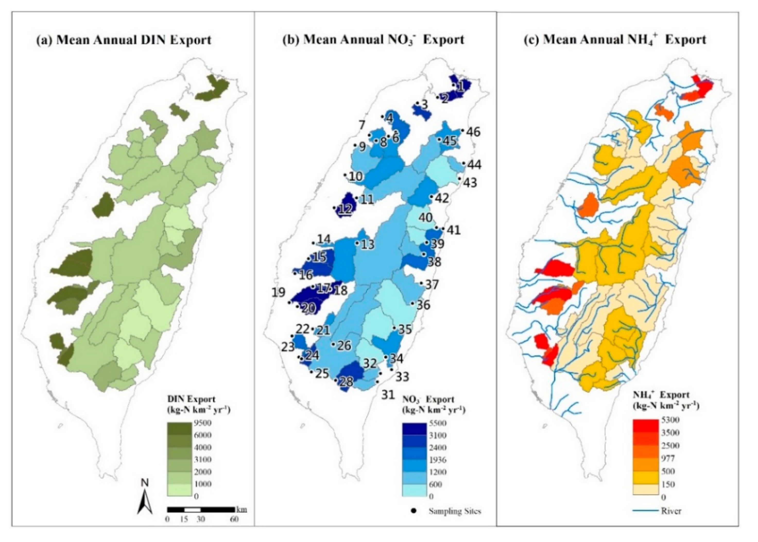
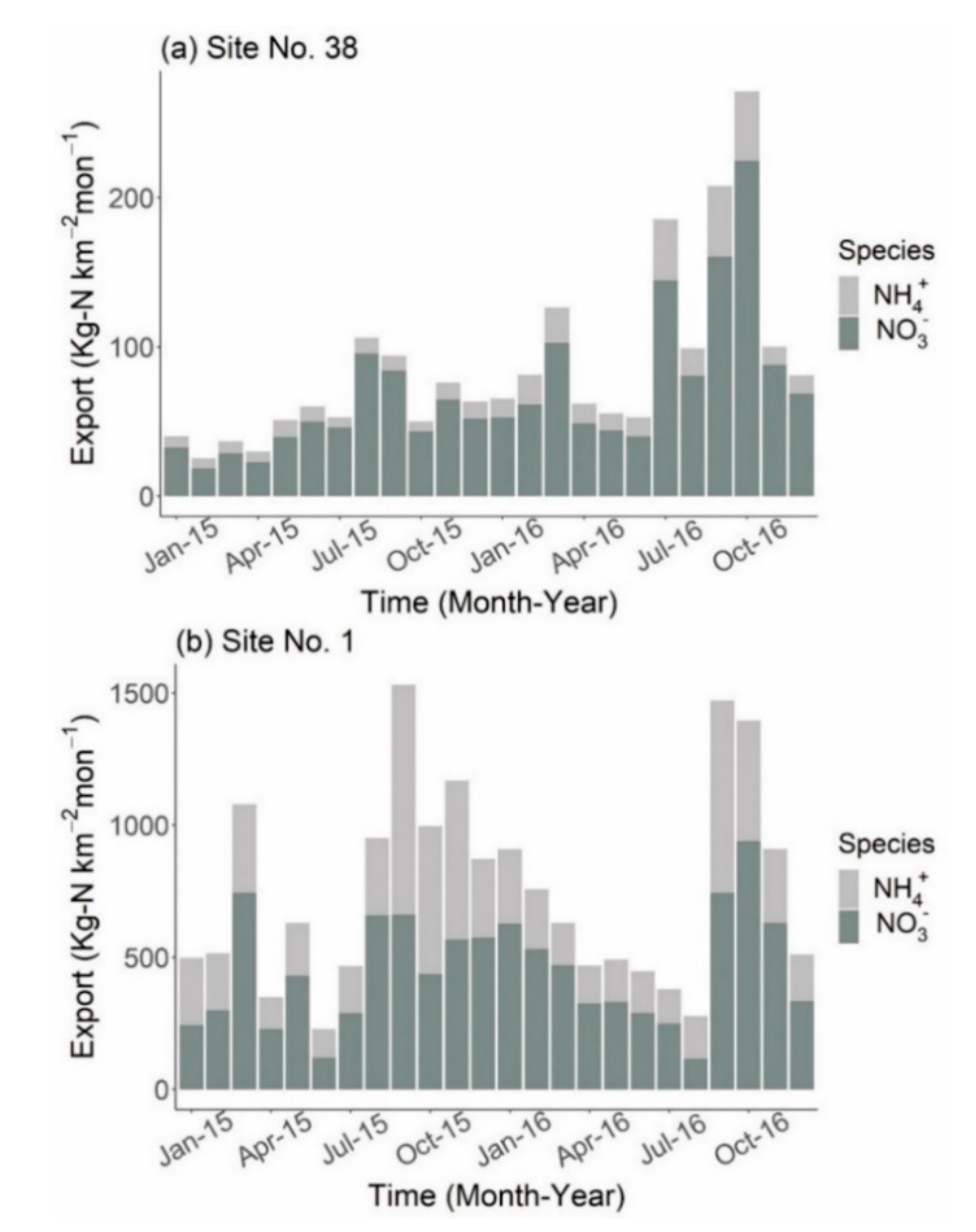
3.1. Riverine DIN Concentration and Export

The mean DIN concentration is 1.66 mg-N L⁻¹, ranging from 0.28 to 8.91 mg-N L⁻¹, while the mean NO₃⁻ concentration is 0.98 mg-N L⁻¹, varying from 0.26 to 2.79 mg-N L⁻¹, and the mean NH₄⁺ concentration is 0.56 mg-N L⁻¹, in the range of 0.01−4.59 mg-N L⁻¹. Generally, the mean NO₃⁻ concentration is higher in the wet season (1.03 mg-N L⁻¹) than in the dry season (0.79 mg-N L⁻¹). In contrast, the mean DIN and NH₄⁺ concentrations have higher values in the dry season (1.82 and 0.95 mg-N L⁻¹) than in the wet season (1.66 and 0.48 mg-N L⁻¹) (

Table 3. Mean estimated seasonal NO₃⁻, NH₄⁺ and dissolved inorganic nitrogen (DIN) concentrations and exports for 43 sampling sites in the study period (unit: mg-N L⁻¹ for conc. and kg-N km⁻² yr⁻¹ for flux).

	Annual		Dry Season		Wet Season
	Conc.	Flux	Conc.	Flux	Conc.	Flux
NO3−
Mean (±SD)	0.98 (±0.59)	1936 (±1363)	0.79 (±0.51)	429 (±520)	1.03 (±0.66)	1507 (±1085)
Min‒Max	0.26−2.79	212−5801	0.14−2.19	7−2917	0.25−3.58	158−4908
NH4+
Mean (±SD)	0.56 (±0.96)	977 (±1456)	0.95 (±1.73)	333 (±551)	0.48 (±0.81)	644 (±950)
Min‒Max	0.01−4.59	9−5757	0.01−9.13	1−2372	0.01−3.81	7−3942
DIN
Mean (±SD)	1.66 (±1.69)	3100 (±2827)	1.82 (±2.07)	798 (±982)	1.66 (±1.74)	2303 (±2041)
Min‒Max	0.28−8.91	227−10,229	0.16−9.74	8−4730	0.28−10.45	185−7527

, Tables S2 and S3). The annual mean DIN export of 43 watersheds island-wide is 3100 kg-N km⁻² yr⁻¹, ranging from 230 to 10,000 kg-N km⁻² yr⁻¹ (Figure 3 and Table 3), in which the highest DIN export (site 16) reaches over 40-fold of the lowest one (site 39; Tables S4 and S5). Generally, watersheds with high DIN, NO₃⁻ and NH₄⁺ concentrations/exports locate in northern and southwestern Taiwan, while watersheds with relatively low DIN, NO₃⁻ and NH₄⁺ concentrations/exports are those in central and eastern Taiwan. However, high NO₃⁻ export does not always correspond to high NH₄⁺ export (e.g., site 41) (Figure 3, Tables S4 and S5). Meanwhile, DIN exports present a significant seasonality that the wet season (from May to October) can contribute over 75% of the annual export on average, and the NO₃⁻ and NH₄⁺ exports during wet and dry seasons also account for 70–80% and 20–30% of annual DIN exports respectively (Tables S4 and S5). However, the contributions of NO₃⁻ and NH₄⁺ for wet and dry seasons to annual DIN export varied among watersheds. For example, the lowest DIN export is 227 kg-N km⁻² yr⁻¹ in site 39, a relatively pristine watershed (87% of forest cover), and the contributions of NO₃⁻ and NH₄⁺ exports in the wet (dry) season to annual DIN export are both 90% (10%). In contrast, the highest DIN export, 10,228 kg-N km⁻² yr⁻¹, appears in site 16, a more disturbed watershed (65% of agricultural land cover), and the contributions of the NO₃⁻ and NH₄⁺ exports in the wet (dry) season to annual DIN export are 85% (15%) and 55% (45%) (Tables S4 and S5).

The compositions of NO₃⁻ and NH₄⁺ between pristine and disturbed watershed (forest cover <50%) varied as well. For instance, in relatively pristine watersheds, such as site 38 (Figure 4a), NO₃⁻ exports were generally higher (~70%) than NH₄⁺ (~20%). On the contrary, NH₄⁺ exports can reach 40% of annual DIN in the higher disturbed watersheds with a smaller drainage area (<1000 km²) and steep slopes (>30%), such as site 1 (Figure 4b). In addition, some watersheds with higher NH₄⁺ exports in lieu of NO₃⁻ are scattered in the plain (slope < 20%) in southwestern Taiwan, such as sites 15, 16 and 22 (Figure 3, Tables S4 and S5).

The average DIN export in 2016 (3460 kg-N km⁻² yr⁻¹) was higher than that in 2015 (2723 kg-N km⁻² yr⁻¹) due to much higher rainfall, 3480 mm in 2016 compared to 2331 mm in 2015 (Tables S4 and S5). The mean NO₃⁻ export in 2016 (2301 kg-N km⁻² yr⁻¹) was higher than in 2015 (1553 kg-N km⁻² yr⁻¹), whereas the mean NH₄⁺ export in 2016 (940 kg-N km⁻² yr⁻¹) was slightly lower than 2015 (1016 kg-N km⁻² yr⁻¹), in which most of the decreased NH₄⁺ exports appeared in watersheds in northern Taiwan, while some NH₄⁺ exports increased in watersheds in southern and eastern Taiwan (Tables S4 and S5).

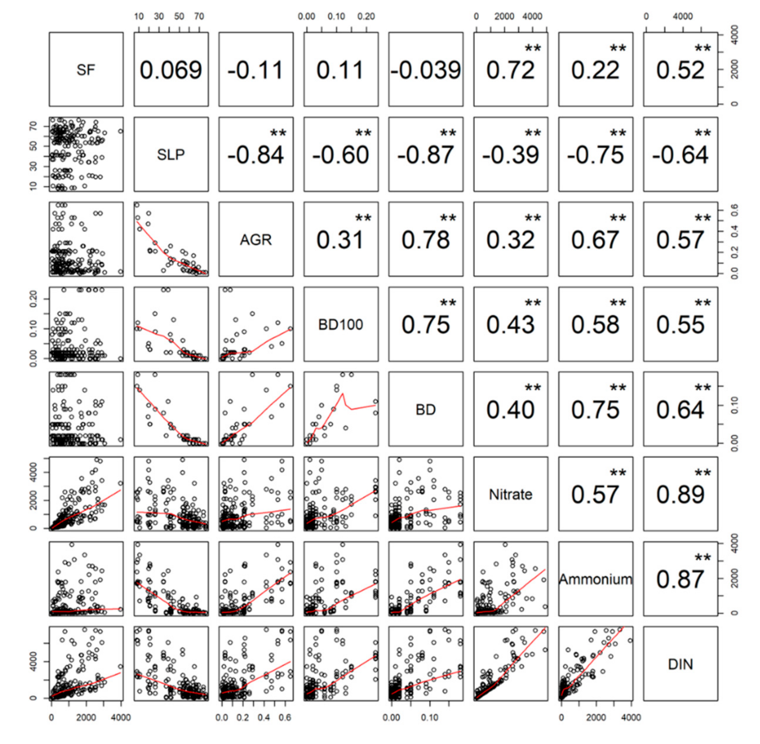
3.2. Scatterplot Matrix

The correlations between nutrient exports and variables at different buffer zones show that significantly higher coefficients are generally found between annual and seasonal nutrient exports and variables at watershed scale (Figures S1–S3), whereas the fraction of buildup area within a 100 m buffer has higher correlations to DIN (r = 0.82, p < 0.01) in the dry season than other variables among different buffer zones (Figure S3). Streamflow, the fraction of agricultural land cover of the entire watershed, buildup area within a 100 m buffer zone and buildup area of the entire watershed show significant positive relationships to DIN export (r = 0.52–0.64, p < 0.01; Figure 5). However, there is a negative relationship found between DIN and slope of entire watershed (r = −0.64, p < 0.01; Figure 5).

Streamflow positively correlates to NO₃⁻ (r = 0.72, p < 0.01) and NH₄⁺ (r = 0.22, p < 0.01; Figure 5). The exports of the two ions also significantly correlate to agriculture, buildup area in a 100 m buffer zone and buildup area within the entire watershed, of which the correlation coefficients are higher in NH₄⁺ (r = 0.58–0.75, p < 0.01; Figure 5) than in NO₃⁻ (r = 0.32–0.43, p < 0.01; Figure 5). However, the slope is negatively significantly related to NO₃⁻ exports (r = −0.39, p < 0.01), NH₄⁺ exports (r = −0.75, p < 0.01), agriculture (r = −0.84, p < 0.01), buildup area within the 100 m buffer zone (r = −0.60, p < 0.01) and buildup area within the entire watershed (r = −0.87, p < 0.01; Figure 5). There are positive correlations among variables of landcover (r = 0.31–0.78, p < 0.01; Figure 5).

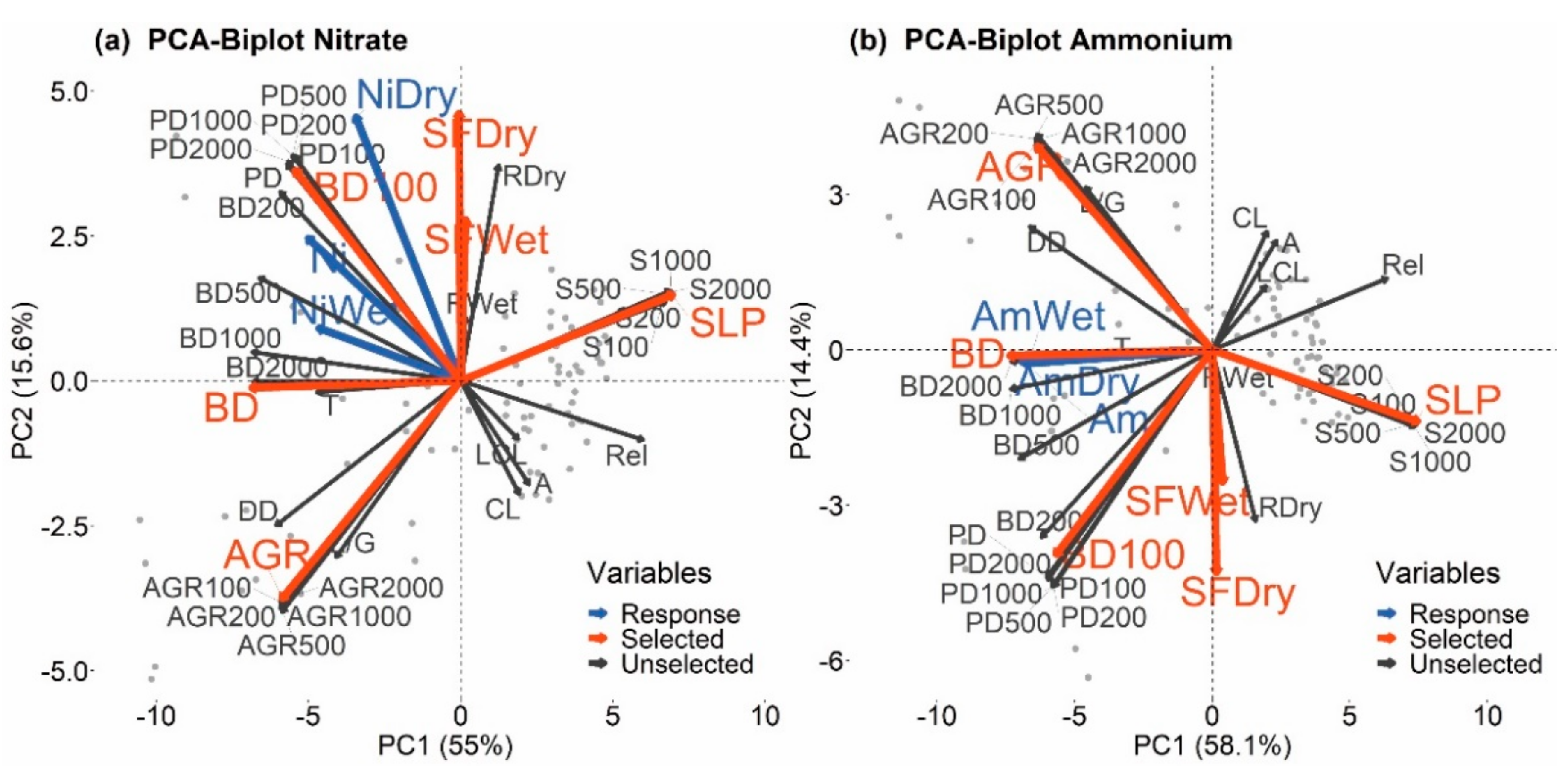
3.3. PCA of Environmental Variables

The first two principal components with eigenvalues > 5.0 are retained, accounting for 70.6% and 72.5% of variances on NO₃⁻ and NH₄⁺ exports, respectively (Figure 6). The combinations of variables within the watershed scale (SF, SLP, AGR, and BD) and buildup area in a 100 m buffer (BD100) can explain much more variances of NO₃⁻ and NH₄⁺ exports than the performance using variables derived from the separate buffer zones (≤60%; Figure S4). Generally, the spatial variability of buildup (BD) and slope (SLP) are the main ingredients of the first PCs for NO₃⁻ and NH₄⁺ (Figure 6). The second PC is associated with seasonal variables, i.e., streamflow (SFWet and SFDry) and rainfall (RWet and RDry) during wet and dry periods. Most environmental variables displayed positive correlations with these two response variables (NO₃⁻ and NH₄⁺), except for landscape setting variables such as area (A), channel length (CL), longest channel length (LCL), relief (R) and slope (SLP), i.e., the opposite direction to NO₃⁻ and NH₄⁺ export (blue lines in Figure 6). During the wet season, the smaller projected angle is between the fraction of BD and NO₃⁻ export (NiWet), indicating high relevance between human impact and the wet season NO₃⁻ export, while during the dry season, NO₃⁻ export relates to the vectors dominated by streamflow and rainfall. However, unlike NO₃⁻ export, NH₄⁺ export is dominated by BD regardless of the different seasons. According to the results derived from PCA, five environmental variables including streamflow, slope, the fraction of agricultural land cover, buildup area within a 100 m buffer zone and buildup area of the entire watershed with higher loading were selected for further analysis.

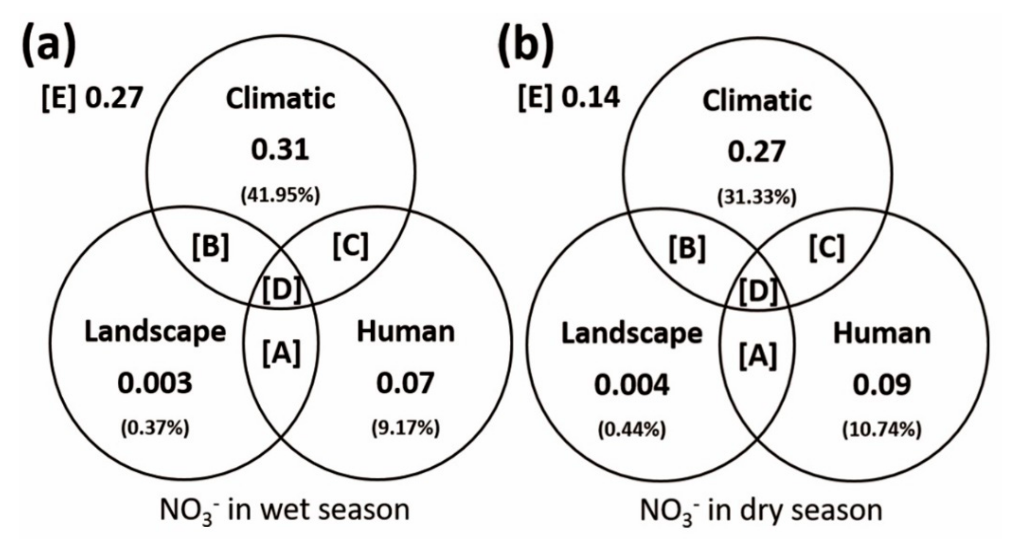
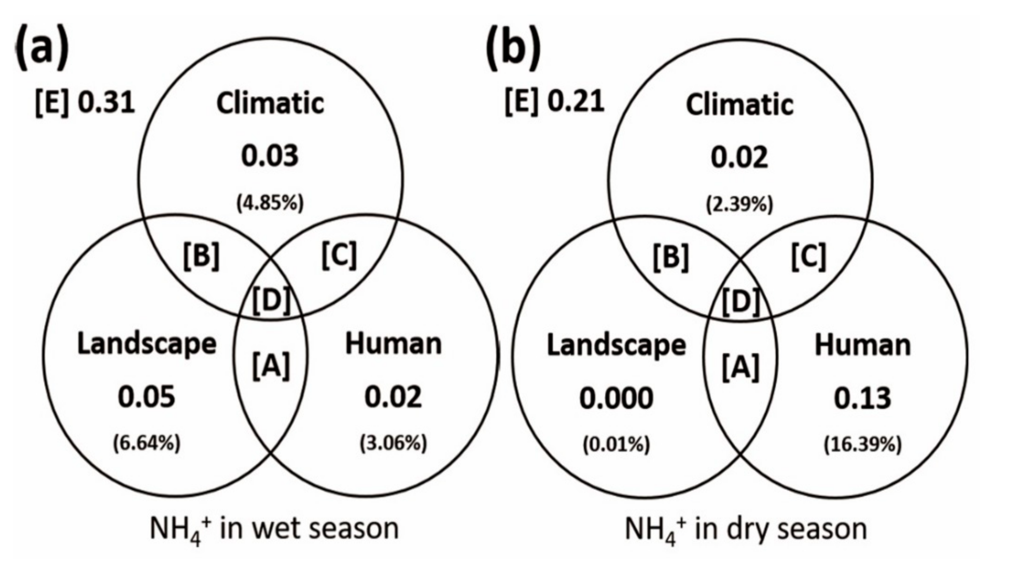
3.4. Variance Partitioning—RDA and pRDA

The RDA model shows that the total variance explained (total inertia) by five selected environmental variables is always higher on NO₃⁻ exports than on NH₄⁺ exports. These predictor variables can explain 86% and 79% of the total variance of NO₃⁻ and NH₄⁺ exports, respectively, in the dry season, but only 73% and 69% in the wet season (

Table 4. The marginal effects (λ₁) and total inertia (total effects) of climatic, landscape setting and human disturbance variables on NO₃⁻ and NH₄⁺ exports based on 43 sampling sites.

Species	NO3−			NH4+
	Annual	Wet	Dry	Annual	Wet	Dry
	λ1	λ1	λ1	λ1	λ1	λ1
Climatic
Streamflow (mm)	0.52 **	0.28 **	0.59 **	0.05 **	0.01 ns	0.02 ns
Landscape setting
Slope (%)	0.15 **	0.32 **	0.12 **	0.56 **	0.64 **	0.61 **
Human disturbance
Agri. (%)	0.11 **	0.31 **	0.01 ns	0.44 **	0.47 **	0.53 **
Buildup_100 m (%)	0.18 **	0.19 **	0.57 **	0.33 **	0.32 **	0.46 **
Buildup (%)	0.16 **	0.26 **	0.21 **	0.57 **	0.58 **	0.73 **
Total inertial	0.74	0.73	0.86	0.68	0.69	0.79

** p < 0.01. ns: not significant.

).

Streamflow reveals the highest marginal effects on NO₃⁻ exports, where marginal effects λ₁ increase from 0.28 in the wet season, 0.52 in annual export, to 0.59 in the dry season. However, the effects of streamflow are low (λ₁ < 0.05) for NH₄⁺ annual and seasonal exports (Table 4). In contrast, slope has lower marginal effects on annual and seasonal NO₃⁻ exports (λ₁ = 0.12–0.32) than on NH₄⁺ exports (λ₁ = 0.56–0.64), and the marginal effects of slope are higher in the wet season (λ₁ = 0.32–0.64) than in the dry season (λ₁ = 0.12–0.61) for nutrient export (Table 4). The anthropogenic factors, including the fraction of agricultural land cover, buildup area within a 100 m buffer and buildup area of the entire watershed, show higher marginal effects on annual and seasonal NH₄⁺ exports (λ₁ = 0.32–0.73) than NO₃⁻ exports (λ₁ = 0.01–0.57), except for fraction of buildup area within a 100 m buffer in the dry season on NO₃⁻ exports (Table 4). Generally, buildup area within a 100 m buffer zone has higher marginal effects on NO₃⁻ exports (λ₁ = 0.18–0.57) than buildup area of entire watershed (λ₁ = 0.16–0.26), although the effect of buildup area within a 100 m buffer is slightly lower (λ₁ = 0.19) than buildup area of entire watershed (λ₁ = 0.26) in the wet season. In the dry season, the effect of buildup area within a 100 m buffer is 2.5 times (λ₁ = 0.57) that of buildup area of entire watershed (λ₁ = 0.21). For NH₄⁺ exports, buildup area of entire watershed has the highest effects (λ₁ = 0.57–0.73) compared with agriculture (λ₁ = 0.44–0.53) and buildup area within a 100 m buffer (λ₁ = 0.32–0.46; Table 4).

For NO₃⁻ exports in pRDA, the lowest (highest) eigenvalue of pure effect on a single variable included is the landscape (climatic) variable in the wet season, 0.003 (0.31), and in the dry season, 0.004 (0.27) (Figure 7). The climatic variable (C) seems to be the dominant factor regarding seasonal NO₃⁻ exports. It is responsible for over 42% and 31% of variance for wet and dry seasonal NO₃⁻ exports (Figure 7). The combination of landscape with human disturbance variables (LH) will contribute a significant effect on NO₃⁻ export in the wet season (0.38 of eigenvalue and 51.59% of explained variance), but decreases substantially in the dry season (0.17 of eigenvalue and 20.00% of explained variance) (Figure 7). While the effects of the combination of climatic with human disturbance variables (CH) increase from 0.04 (5.32% of explained variance) in the wet season (Figure 7a) to 0.38 (44.15% of explained variance) in the dry season (Figure 7b).

For NH₄⁺ exports in pRDA, the eigenvalues of each single variable (pure effect) are lower than 0.05 (Figure 8). The only exception is the pure effect on human disturbance variables in the dry season (H = 0.13), which accounts for 16.4% of explained variance (Figure 8). The dominant effect is the combination of landscape with human disturbance variables (LH) in which eigenvalues reach 0.61 (88.5%) and 0.64 (80.7%) of the total NH₄⁺ export variance in the wet and dry season, respectively (Figure 8). Other interactive effects are much lower than LH in both seasons.

4. Discussion

4.1. Characteristics of DIN Concentrations and Exports in Taiwan

On average, DIN concentration from 43 island-wide watersheds across Taiwan is 1.66 mg-N L⁻¹, and the two main DIN species present a mediated dilution effect with streamflow (Table 3 and Figure S5). The average riverine DIN export reaches 3100 kg-N km⁻² yr⁻¹, which is much greater than the global mean (208 kg-N km⁻² yr⁻¹) [12]. High rainfall and streamflow, N deposition and N fertilizer application for agricultural production at upstream regions can account for the significant nutrients streamflow [11]. The results reveal that DIN export and concentration vary spatially, ranging from 200 kg-N km⁻² yr⁻¹, 0.3 mg-N L⁻¹ in less disturbed watersheds (site 39; Figure 3), to over 10,000 kg-N km⁻² yr⁻¹, 8.8 mg-N L⁻¹ in highly disturbed watersheds (site 16; Figure 3). The spatial DIN surge also indicates that the environmental background actually exports DIN and consequently induces the risk of eutrophication in the downstream. Previous studies suggested that intact forested watersheds demonstrated high N retention capacity but the capacity would collapse with significant land cover conversion [16,40]. In our study, higher NH₄⁺ exports in highly disturbed watersheds with smaller drainage area (<1000 km²) and steep slope (>30%) show that these environmental backgrounds are unfavorable to ammonia oxidation or assimilation due to rapid transport [41]. In addition, most of the watersheds with higher NH₄⁺ exports than NO₃⁻ appear in plain areas where human disturbances are high and sewage systems are deficient [42].

The island-wide DIN estimation reveals that the wet season (May to October) contributes 78% of the annual DIN export, 3100 kg-N km⁻² yr⁻¹, which is consistent with previous findings that hydrological processes control DIN export [43,44]. Because nutrient export and transport is regulated by precipitation and streamflow, this controlling factor is more dominant in the tropics and subtropics [12,45]. The torrential rainfall brought by typhoons during the humid growing summer in Taiwan accounts for 30−50% of the annual precipitation, 2500 mm yr⁻¹ [13,46], and consequently causes vital effects on biogeochemical processes, i.e., a huge amount of nutrients being flushed out from terrestrial ecosystems to aquatic ecosystems. It also explains why the nutrient streamflow in Taiwan is in the leading place worldwide [12].

4.2. Influences of Main Variables and Their Interactive Effects on DIN Export

4.2.1. Climatic Control

In tropical/subtropical mountainous Taiwan, abundant rainfall usually leads to a great amount of net nutrient exports even during the growing summer, which is distinct from the findings in temperate forest ecosystems [11,45,47]. Water is the conveyor of ion movement. In spite of the dilution of NO₃⁻ concentration during flood periods (wet season), the extensive runoff by typhoons flushes over surface and near-surface and leads to greater DIN exports [13].

The relation between export and streamflow (F-Q relation), which definitely shows export change with streamflow, is particularly crucial as regarding nutrient balance and transport, although the F-Q relation, which inevitably incorporates streamflow in the calculation, could likely lead to the “spurious relation”. However, the F-Q relation, which can present the dominance of supply-limited or kinetically-limited under different hydrologic conditions, helps to indicate the nutrient budget balance, and the transported amount is also important. Notably, there are totally different hydrological controls on NO₃⁻ and NH₄⁺ transport. One is that streamflow plays a strong role on NO₃⁻ export (r = 0.72; λ₁ = 0.28–0.59), which is in contrast to a relatively weak relation with NH₄⁺ export (r = 0.22; λ₁ < 0.05). The positive NO₃⁻ streamflow relation indicates the sources are relatively sufficient, as compared to kinetic transport. One possible interpretation is that warmer and more humid conditions (e.g., higher soil moisture) during the wet summer season are favorable for nitrification and promotes NO₃⁻ accumulation and then transports it from the soil to the aquatic system [48,49]. On the contrary, NH₄⁺ is easily converted and emitted to the atmosphere via microbial activities in warm and humid conditions [15,50], which has lower retention in soil capacity compared to NO₃⁻. Whether NH₄⁺ is source-limited casts a shadow of doubt on hydrologic control on NH₄⁺ transport.

4.2.2. The Consideration of Landscape and Buffer Zone

Streams receive nutrients from aquatic ecosystems and adjacent terrestrial landscapes, such that landscape configuration at watershed- or buffer zone-scale has important influences on stream water quality, ecological process and biodiversity. Watersheds with steeper slopes usually export more nutrients [51], yet our results surprisingly show that slope is negatively related to NO₃⁻ and NH₄⁺ exports (Figure 5). The possible reason is that most upstream watersheds with steep slopes are covered by pristine forests where anthropogenic sources are scarce [10,52]. Studies suggested that elevation might be a suitable parameter to predict water quality [30], but the collinearity between landscape (e.g., elevation or SLP) and human-made land cover (e.g., AGR and BD) from the high, steep montane region to the low, flat plain in Taiwan keeps us from using both simultaneously, even they might have significant contribution on nutrient exports.

Many studies demonstrate the control of land use and landscape on water quality at watershed scale [28,30], but few studies consider the distance from source area to river, i.e., the regulation of the riparian or buffer zone on nutrient movement. Plants and microbial activities within the riparian zone can help to uptake a great quantity of water, nutrients and sediments, mitigating the nutrients export to aquatic ecosystems within the watershed [53,54]. However, the effective buffer distance is uncertain, and it could vary with the elements which are concerned [36,55]. A study conducted in Puerto Rico examined how the landscape pattern changes affected water quality in-stream and found that turbidity and dissolved oxygen responded to land use and land cover (LUC) at watershed scale [35], phosphorus concentration and fecal matter responded to LUC at sub-watershed scale, whereas nitrogen concentrations linked to LUC in riparian buffers of larger watersheds [35]. Another study conducted in the Saginaw Bay of central Michigan investigating 62 catchments with a gradient of disturbed land cover showed that the land use factors within a 100 m buffer zone adjacent to the river could explain much higher (or equal) variance of NO₃⁻ and NH₄⁺ concentrations than those derived from the watershed scale [52]. Conversely, the relationships between total nitrogen exports and land use at the watershed scale were better than riparian buffer zones of 200 and 400 m in highly disturbed rivers in Illinois and Texas [56]. Previous assessments, based upon mountainous background, demonstrated that the buffer zone within a 100 m riparian zone, the buildup area particularly, plays an important role in regulating DIN exports [56,57,58]. In Taiwan, the deficiency of sewage systems in buildup areas located near river networks contributes a significant amount to the DIN exports [42]. The percentage of buildup at the watershed scale highlighted in our study indicates that dispersal non-point sewage sources in the buildup area and scattered agricultural activities would be critical in assessing NH₄⁺ export.

4.2.3. Human Disturbance

The contribution of human activities to DIN exports (including NO₃⁻ and NH₄⁺) from land to water has been underscored due to agricultural activities (e.g., fertilizer application) and urbanization (e.g., domestic wastewater) [52,59]. To meet the ever-increasing demand, agricultural activities, such as high value fruit, montane cabbage and tea plantations, are pervasive in mountainous Taiwan. Consequently, the excessive addition of inorganic N fertilizer and organic manure on the thin soil layer is readily flushed out to aquatic ecosystems downstream during wet season [12,60]. The N retention or removal capacity within watersheds will dramatically decrease if forests are transformed to agricultural areas [61]. However, though the effects of agricultural land on NO₃⁻ and NH₄⁺ exports are statistically significant, their contributions are weaker than previous studies suggested [57,58]. A Canadian study suggested that urban land use has a stronger effect on water quality than agriculture has [14]. Obviously, the importance of agricultural and urban land use on DIN exports is not easy to identify and separate, not only due to the area, but also the “intensity” (e.g., intensive agriculture or dense population) and spatial configuration. For example, the effect of urban areas is minor in Finland, because the population and settlements are mostly scattered so that wastewater can be purified before it flows into main streams [28].

In this study, both NO₃⁻ and NH₄⁺ exports are significantly correlated to AGR and BD, which shows that AGR and BD are important for DIN exports (Figure 5). Notably, higher correlation coefficients of AGR and BD to NH₄⁺ export (r = 0.67–0.75) than those to NO₃⁻ export (r = 0.32–0.40) indicates that land use pattern is more effective to explain the variance of NH₄⁺ export. Conceptually, NH₄⁺ is easier to be taken up by plants and to be oxidized through nitrification and thus NO₃⁻ is the main species of DIN within agriculture-dominated catchments. The intensive urban developments located near stream riparian in Taiwan deteriorates water quality directly and contributes a significant amount to the DIN exports. This phenomenon is reflected by the higher effect of BD100 (buildup area in a 100 m buffer zone) than the BD of the entire watershed on NO₃⁻ export during the dry season (Table 4). Therefore, domestic wastewater inevitably elevates NH₄⁺ export, which indicates a strong intrinsic collinearity with agriculture and buildup area. Such intrinsic collinearity presents an inseparable human-landscape system, and their interplay could not be distinguished perfectly.

4.2.4. Interactive Effects among Variables

It was noticeable that interactive effects between landscape and human variables can explain most variabilities of NO₃⁻ export in the wet season (51.59% of the total variance) and seasonal NH₄⁺ export (both >80% of the total variance). Meanwhile, interactive effects between climatic and human variables explain 44.15% of the total NO₃⁻ export variance in the dry season. Thus, the interactive effect between landscape setting and human disturbance and climatic and human disturbance will result in a high efficiency of prediction regarding NO₃⁻ and NH₄⁺ export in different conditions. One explanatory variable might be partially linked to other variables and altogether would improve or reduce the predictive power in evaluation of NO₃⁻ and NH₄⁺ export [62]. For example, the opposite influences of streamflow and slope might suppress their capability to assess NO₃⁻ and NH₄⁺ exports without eliminating the collinearity between them. The mixed effects of environmental variables also suggest that it is necessary and will be more effective to apply an integrative management strategy [63].

There is a significant change between the controlling interactive effects of NO₃⁻ export in the wet and dry seasons. In the wet season, streamflow and interactive effects between landscape setting and human disturbance might reveal that they are two unique groups controlling the variance of NO₃⁻ export. This might be reasonable because the abundant rainfall during the humid summer will decrease the spatial variability of streamflow across Taiwan, which leads to a weaker relationship between streamflow and the interactive effects of landscape setting and human disturbance. On the contrary, the increase of the interactive effects between climatic and human disturbance might indicate the increasing spatial variability of streamflow in the dry season. Therefore, when we predict NO₃⁻ export in the wet season, both streamflow and the interactive effects between landscape setting and human disturbance cannot be ignored. Furthermore, the strong interactive effects between landscape setting and human disturbance on NH₄⁺ export, indicates that these two groups are the primary control of NH₄⁺ export. Because landscape setting and human disturbance are highly related (Figure 5), the variance explained by them might be similar and it might be difficult to separate their individual effect from both combined.

Some critical variables are not included in this study but might be significant in other regions. Studies found a strong negative relationship between nitrogen content and soil type [14]. However, most watersheds in Taiwan cross various soil substrates and geological units, which challenges us to unambiguously define a specific soil type for each watershed. In addition, long-lasting atmospheric nitrogen deposition could lead to N saturation in temperate forest ecosystems, resulting in net loss of nitrate to streams and consequent acidification of stream water [1,16,64]. A large-scale study indicated that riverine N export could be predicted by atmospheric N deposition rates [65]. Therefore, the influence of interaction between atmospheric deposition, land use and hydroclimate should be considered in following syntheses of DIN responses or developing models for riverine DIN export [66].

5. Conclusions

This work identified the major predictor variables and their interactive effects on DIN, NO₃⁻ and NH₄⁺ exports. Totally, 35 predictor variables among climatic, landscape setting and human disturbance dimensions were applied using PCA and pRDA analysis based upon data derived from 43 watersheds island-wide in Taiwan. Generally, the PCA identified that SF, SLP, AGR, BD and BD100 are the main variables which can mostly explain the variances of DIN, NO₃⁻ and NH₄⁺ exports. Because nutrient export is the product of nutrient concentration and streamflow, streamflow, as expected, is the strongest predictor for NO₃⁻ export (r = 0.72), but not for NH₄⁺ export, due to active biogeochemical processes. Meanwhile, the SLP (r = 0.75) and BD (r = −0.75) are equally best correlated to NH₄ export. Based on the results of the pRDA model, five selected environmental variables can explain NO₃ and NH₄⁺ export promisingly, but with different interactive effects. For NO₃⁻ export in the wet season, the climatic variable and human-landscape variables are independently responsive to most variances, while the dependent climatic-human variables present high marginal effects on NO₃⁻ exports in the dry season. The effective variables shift from human-landscape to climatic-human with seasons showing the mechanistic shift of nutrient transport. For NH₄⁺ export, the residual variances are 0.31 and 0.21 for the wet and dry seasons, respectively, and climatic variables (e.g., streamflow) are not effective variables for NH₄⁺ transport. The human-landscape variables are the major factors to explain the total variance of NH₄⁺ export (over 80%), in both the wet and dry seasons. The shift of interactive effects of variables on nutrient export is important for water quality management at watershed scale and designing mitigation strategies. Inevitably, the effects of intrinsic collinearity in the human-landscape system cannot be clearly separated due to spurious correlation, though the statistical approach provides some cues. For example, paired AGR and BD or SLP and BD are highly collinear but difficult to single out for estimating nutrient export and for interpretation. Nevertheless, with the accumulation of these studies, it is more possible to clarify the interactive effects, which could be of great help in advancing the understanding of DIN export mechanisms and global synthesized assessment.

References

1. Aber, J.; McDowell, W.; Nadelhoffer, K.; Magill, A.; Berntson, G.; Kamakea, M.; McNulty, S.; Currie, W.; Rustad, L.; Fernandez, I. Nitrogen saturation in temperate forest ecosystems: Hypotheses revisited. Bioscience 1998, 48, 921–934. [Google Scholar] [CrossRef]
2. Galloway, J.N.; Dentener, F.J.; Capone, D.G.; Boyer, E.W.; Howarth, R.W.; Seitzinger, S.P.; Asner, G.P.; Cleveland, C.C.; Green, P.; Holland, E.A. Nitrogen cycles: Past, present, and future. Biogeochemistry 2004, 70, 153–226. [Google Scholar] [CrossRef]
3. Seitzinger, S.P.; Mayorga, E.; Bouwman, A.F.; Kroeze, C.; Beusen, A.H.W.; Billen, G.; Van Drecht, G.; Dumont, E.; Fekete, B.M.; Garnier, J.; et al. Global river nutrient export: A scenario analysis of past and future trends. Glob. Biogeochem. Cycle 2010, 24, GB0A08. [Google Scholar] [CrossRef] [Green Version]
4. Rockström, J.; Steffen, W.; Noone, K.; Persson, Å.; Chapin, F.S.; Lambin, E.F.; Lenton, T.M.; Scheffer, M.; Folke, C.; Schellnhuber, H.J. A safe operating space for humanity. Nature 2009, 461, 472–475. [Google Scholar] [CrossRef] [PubMed]
5. Tørseth, K.; Aas, W.; Breivik, K.; Fjæraa, A.M.; Fiebig, M.; Hjellbrekke, A.-G.; Lund Myhre, C.; Solberg, S.; Yttri, K.E. Introduction to the European Monitoring and Evaluation Programme (EMEP) and observed atmospheric composition change during 1972–2009. Atmos. Chem. Phys. 2012, 12, 5447–5481. [Google Scholar] [CrossRef] [Green Version]
6. Vet, R.; Artz, R.S.; Carou, S.; Shaw, M.; Ro, C.-U.; Aas, W.; Baker, A.; Bowersox, V.C.; Dentener, F.; Galy-Lacaux, C. A global assessment of precipitation chemistry and deposition of sulfur, nitrogen, sea salt, base cations, organic acids, acidity and pH, and phosphorus. Atmos. Environ. 2014, 93, 3–100. [Google Scholar] [CrossRef]
7. Chang, K.-H.; Jeng, F.-T.; Tsai, Y.-L.; Lin, P.-L. Modeling of long-range transport on Taiwan’s acid deposition under different weather conditions. Atmos. Environ. 2000, 34, 3281–3295. [Google Scholar] [CrossRef]
8. Conley, D.J.; Paerl, H.W.; Howarth, R.W.; Boesch, D.F.; Seitzinger, S.P.; Havens, K.E.; Lancelot, C.; Likens, G.E. Controlling eutrophication: Nitrogen and phosphorus. Science 2009, 323, 1014–1015. [Google Scholar] [CrossRef]
9. Howarth, R.; Swaney, D.; Billen, G.; Garnier, J.; Hong, B.; Humborg, C.; Johnes, P.; Mörth, C.-M.; Marino, R. Nitrogen fluxes from the landscape are controlled by net anthropogenic nitrogen inputs and by climate. Front. Ecol. Environ. 2012, 10, 37–43. [Google Scholar] [CrossRef] [Green Version]
10. Chang, C.T.; Huang, J.C.; Wang, L.; Shih, Y.T.; Lin, T.C. Shifts in stream hydrochemistry in responses to typhoon and non-typhoon precipitation. Biogeosciences 2018, 15, 2379–2391. [Google Scholar] [CrossRef] [Green Version]
11. Huang, J.-C.; Lee, T.-Y.; Kao, S.-J.; Hsu, S.-C.; Lin, H.-J.; Peng, T.-R. Land use effect and hydrological control on nitrate yield in subtropical mountainous watersheds. Hydrol. Earth Syst. Sci. 2012, 16, 699. [Google Scholar] [CrossRef] [Green Version]
12. Huang, J.-C.; Lee, T.-Y.; Lin, T.-C.; Hein, T.; Lee, L.-C.; Shih, Y.-T.; Kao, S.-J.; Shiah, F.-K.; Lin, N.-H. Effects of different N sources on riverine DIN export and retention in a subtropical high-standing island, Taiwan. Biogeosciences 2016, 13, 1787. [Google Scholar] [CrossRef] [PubMed] [Green Version]
13. Lee, T.-Y.; Huang, J.-C.; Kao, S.-J.; Tung, C.-P. Temporal variation of nitrate and phosphate transport in headwater catchments: The hydrological controls and land use alteration. Biogeosciences 2013, 10, 2617–2632. [Google Scholar] [CrossRef] [Green Version]
14. Sliva, L.; Williams, D.D. Buffer zone versus whole catchment approaches to studying land use impact on river water quality. Water Res. 2001, 35, 3462–3472. [Google Scholar] [CrossRef]
15. Pajares, S.; Bohannan, B.J. Ecology of nitrogen fixing, nitrifying, and denitrifying microorganisms in tropical forest soils. Front. Microbiol. 2016, 7, 1045. [Google Scholar] [CrossRef] [Green Version]
16. Howarth, R.W. An assessment of human influences on fluxes of nitrogen from the terrestrial landscape to the estuaries and continental shelves of the North Atlantic Ocean. Nutr. Cycl. Agroecosyst. 1998, 52, 213–223. [Google Scholar] [CrossRef]
17. Graham, M.H. Confronting multicollinearity in ecological multiple regression. Ecology 2003, 84, 2809–2815. [Google Scholar] [CrossRef] [Green Version]
18. Ter Braak, C.J. CANOCO-a FORTRAN Program. for Canonical Community Ordination by [Partial][Etrended][Canonical] Correspondence Analysis, Principal Components Analysis and Redundancy Analysis (Version 2.1); Wageningen University: Wageningen, The Netherlands, 1988. [Google Scholar]
19. Borcard, D.; Legendre, P.; Drapeau, P. Partialling out the spatial component of ecological variation. Ecology 1992, 73, 1045–1055. [Google Scholar] [CrossRef] [Green Version]
20. Chang, C.-T.; Wang, S.-F.; Vadeboncoeur, M.A.; Lin, T.-C. Relating vegetation dynamics to temperature and precipitation at monthly and annual timescales in Taiwan using MODIS vegetation indices. Int. J. Remote Sens. 2014, 35, 598–620. [Google Scholar] [CrossRef]
21. Parajka, J.; Viglione, A.; Rogger, M.; Salinas, J.L.; Sivapalan, M.; Blöschl, G. Comparative assessment of predictions in ungauged basins–Part 1: Runoff-hydrograph studies. Hydrol. Earth Syst. Sci. 2013, 17, 1783–1795. [Google Scholar] [CrossRef] [Green Version]
22. Huang, J.-C.; Kao, S.-J.; Lin, C.-Y.; Chang, P.-L.; Lee, T.-Y.; Li, M.-H. Effect of subsampling tropical cyclone rainfall on flood hydrograph response in a subtropical mountainous catchment. J. Hydrol. 2011, 409, 248–261. [Google Scholar] [CrossRef]
23. Nash, J.E.; Sutcliffe, J.V. River flow forecasting through conceptual models part I—A discussion of principles. J. Hydrol. 1970, 10, 282–290. [Google Scholar] [CrossRef]
24. Appling, A.P.; Leon, M.C.; McDowell, W.H. Reducing bias and quantifying uncertainty in watershed flux estimates: The R package loadflex. Ecosphere 2015, 6, 1–25. [Google Scholar] [CrossRef]
25. Porterfield, G. Computation of Fluvial-Sediment Discharge; US Government Printing Office: Washington, DC, USA, 1972. [Google Scholar] [CrossRef]
26. Robertson, D.M.; Roerish, E.D. Influence of various water quality sampling strategies on load estimates for small streams. Water Resour. Res. 1999, 35, 3747–3759. [Google Scholar] [CrossRef]
27. Ferguson, R. River loads underestimated by rating curves. Water Resour. Res. 1986, 22, 74–76. [Google Scholar] [CrossRef]
28. Varanka, S.; Luoto, M. Environmental determinants of water quality in boreal rivers based on partitioning methods. River Res. Appl. 2012, 28, 1034–1046. [Google Scholar] [CrossRef]
29. Liu, Q. Variation partitioning by partial redundancy analysis (RDA). Environmetrics 1997, 8, 75–85. [Google Scholar] [CrossRef]
30. Nava-López, M.Z.; Diemont, S.A.; Hall, M.; Ávila-Akerberg, V. Riparian buffer zone and whole watershed influences on river water Quality: Implications for ecosystem services near megacities. Environ. Process. 2016, 3, 277–305. [Google Scholar] [CrossRef]
31. Johnson, R.K.; Furse, M.T.; Hering, D.; Sandin, L. Ecological relationships between stream communities and spatial scale: Implications for designing catchment-level monitoring programmes. Freshw. Biol. 2007, 52, 939–958. [Google Scholar] [CrossRef]
32. Jolliffe, I.T.; Cadima, J. Principal component analysis: A review and recent developments. Philos. Trans. R. Soc. A 2016, 374, 20150202. [Google Scholar] [CrossRef]
33. Hotelling, H. Analysis of a complex of statistical variables into principal components. J. Educ. Psychol. 1933, 24, 417. [Google Scholar] [CrossRef]
34. Sutter, J.M.; Kalivas, J.H. Comparison of forward selection, backward elimination, and generalized simulated annealing for variable selection. Microchem. J. 1993, 47, 60–66. [Google Scholar] [CrossRef]
35. Uriarte, M.; Yackulic, C.B.; Lim, Y.; Arce-Nazario, J.A. Influence of land use on water quality in a tropical landscape: A multi-scale analysis. Landsc. Ecol. 2011, 26, 1151. [Google Scholar] [CrossRef] [Green Version]
36. Nielsen, A.; Trolle, D.; Søndergaard, M.; Lauridsen, T.L.; Bjerring, R.; Olesen, J.E.; Jeppesen, E. Watershed land use effects on lake water quality in Denmark. Ecol. Appl. 2012, 22, 1187–1200. [Google Scholar] [CrossRef] [PubMed]
37. Xiao, R.; Wang, G.; Zhang, Q.; Zhang, Z. Multi-scale analysis of relationship between landscape pattern and urban river water quality in different seasons. Sci. Rep. 2016, 6, 1–10. [Google Scholar] [CrossRef] [PubMed] [Green Version]
38. legendre, P.; legendre, L. Chapter 9—Ordination in reduced space. In Developments in Environmental Modelling; Legendre, P., Legendre, L., Eds.; Elsevier: Amsterdam, The Netherlands, 2012; Volume 24, pp. 425–520. [Google Scholar]
39. Legendre, P.; Oksanen, J.; ter Braak, C.J. Testing the significance of canonical axes in redundancy analysis. Methods Ecol. Evol. 2011, 2, 269–277. [Google Scholar] [CrossRef]
40. Groffman, P.M.; Law, N.L.; Belt, K.T.; Band, L.E.; Fisher, G.T. Nitrogen fluxes and retention in urban watershed ecosystems. Ecosystems 2004, 7, 393–403. [Google Scholar] [CrossRef]
41. Halbfaß, S.; Gebel, M.; Bürger, S. Modelling of long term nitrogen retention in surface waters. Adv. Geosci. 2010, 27, 145–148. [Google Scholar] [CrossRef] [Green Version]
42. Lee, T.-Y.; Shih, Y.-T.; Huang, J.-C.; Kao, S.-J.; Shiah, F.-K.; Liu, K.-K. Speciation and dynamics of dissolved inorganic nitrogen export in the Danshui River, Taiwan. Biogeosciences Discuss. 2014, 11, 5307–5321. [Google Scholar] [CrossRef] [Green Version]
43. He, B.; Kanae, S.; Oki, T.; Hirabayashi, Y.; Yamashiki, Y.; Takara, K. Assessment of global nitrogen pollution in rivers using an integrated biogeochemical modeling framework. Water Res. 2011, 45, 2573–2586. [Google Scholar] [CrossRef]
44. Ohowa, B.; Mwashote, B.; Shimbira, W. Dissolved inorganic nutrient fluxes from two seasonal rivers into Gazi Bay, Kenya. Estuar. Coast. Shelf Sci. 1997, 45, 189–195. [Google Scholar] [CrossRef]
45. Chang, C.-T.; Wang, L.-J.; Huang, J.-C.; Liu, C.-P.; Wang, C.-P.; Lin, N.-H.; Wang, L.; Lin, T.-C. Precipitation controls on nutrient budgets in subtropical and tropical forests and the implications under changing climate. Adv. Water Resour. 2017, 103, 44–50. [Google Scholar] [CrossRef] [Green Version]
46. Chang, C.; Hamburg, S.; Hwong, J.; Lin, N.; Hsueh, M.; Chen, M.; Lin, T.-C. Impacts of tropical cyclones on hydrochemistry of a subtropical forest. Hydrol. Earth Syst. Sci. 2013, 17, 3815. [Google Scholar] [CrossRef] [Green Version]
47. Likens, G.E. Biogeochemistry of a Forested Ecosystem; Springer: Berlin/Heidelberg, Germany, 2013. [Google Scholar] [CrossRef]
48. Goodale, C.L.; Thomas, S.A.; Fredriksen, G.; Elliott, E.M.; Flinn, K.M.; Butler, T.J.; Walter, M.T. Unusual seasonal patterns and inferred processes of nitrogen retention in forested headwaters of the Upper Susquehanna River. Biogeochemistry 2009, 93, 197–218. [Google Scholar] [CrossRef]
49. Ohte, N. Implications of seasonal variation in nitrate export from forested ecosystems: A review from the hydrological perspective of ecosystem dynamics. Ecol. Res. 2012, 27, 657–665. [Google Scholar] [CrossRef]
50. Lladó, S.; López-Mondéjar, R.; Baldrian, P. Forest Soil Bacteria: Diversity, Involvement in Ecosystem Processes, and Response to Global Change. Microbiol. Mol. Biol. Rev. 2017, 81, e00063–16. [Google Scholar] [CrossRef] [Green Version]
51. Richards, C.; Johnson, L.B.; Host, G.E. Landscape-scale influences on stream habitats and biota. Can. J. Fish. Aquat. Sci. 1996, 53, 295–311. [Google Scholar] [CrossRef]
52. Johnson, L.; Richards, C.; Host, G.; Arthur, J. Landscape influences on water chemistry in Midwestern stream ecosystems. Freshw. Biol. 1997, 37, 193–208. [Google Scholar] [CrossRef]
53. Craig, L.S.; Palmer, M.A.; Richardson, D.C.; Filoso, S.; Bernhardt, E.S.; Bledsoe, B.P.; Doyle, M.W.; Groffman, P.M.; Hassett, B.A.; Kaushal, S.S. Stream restoration strategies for reducing river nitrogen loads. Front. Ecol. Environ. 2008, 6, 529–538. [Google Scholar] [CrossRef] [Green Version]
54. Kaushal, S.S.; Groffman, P.M.; Mayer, P.M.; Striz, E.; Gold, A.J. Effects of stream restoration on denitrification in an urbanizing watershed. Ecol. Appl. 2008, 18, 789–804. [Google Scholar] [CrossRef] [Green Version]
55. Gergel, S.E.; Turner, M.G.; Kratz, T.K. Dissolved organic carbon as an indicator of the scale of watershed influence on lakes and rivers. Ecol. Appl. 1999, 9, 1377–1390. [Google Scholar] [CrossRef]
56. Hunsaker, C.T.; Levine, D.A. Hierarchical approaches to the study of water quality in rivers. Bioscience 1995, 45, 193–203. [Google Scholar] [CrossRef]
57. Meynendonckx, J.; Heuvelmans, G.; Muys, B.; Feyen, J. Effects of watershed and riparian zone characteristics on nutrient concentrations in the River Scheldt Basin. Hydrol. Earth Syst. Sci. 2006, 10, 913–922. [Google Scholar] [CrossRef] [Green Version]
58. Tong, S.T.; Chen, W. Modeling the relationship between land use and surface water quality. J. Environ. Manag. 2002, 66, 377–393. [Google Scholar] [CrossRef] [PubMed]
59. Basnyat, P.; Teeter, L.D.; Flynn, K.M.; Lockaby, B.G. Relationships between landscape characteristics and nonpoint source pollution inputs to coastal estuaries. Environ. Manag. 1999, 23, 539–549. [Google Scholar] [CrossRef]
60. Chang, M.; McCullough, J.D.; Granillo, A.B. Effects of land use and topography on some water quality variables in forested east Texas 1. J. Am. Water Resour. Assoc. 1983, 19, 191–196. [Google Scholar] [CrossRef]
61. Shih, Y.-T.; Lee, T.-Y.; Huang, J.-C.; Kao, S.-J. Apportioning riverine DIN load to export coefficients of land uses in an urbanized watershed. Sci. Total Environ. 2016, 560, 1–11. [Google Scholar] [CrossRef]
62. Hough-Snee, N.; Roper, B.; Wheaton, J.; Lokteff, R. Riparian vegetation communities of the American Pacific Northwest are tied to multi-scale environmental filters. River Res. Appl. 2015, 31, 1151–1165. [Google Scholar] [CrossRef]
63. Aschonitis, V.; Feld, C.; Castaldelli, G.; Turin, P.; Visonà, E.; Fano, E.A. Environmental stressor gradients hierarchically regulate macrozoobenthic community turnover in lotic systems of Northern Italy. Hydrobiologia 2016, 765, 131–147. [Google Scholar] [CrossRef]
64. Aber, J.D.; Nadelhoffer, K.J.; Steudler, P.; Melillo, J.M. Nitrogen saturation in northern forest ecosystems. Bioscience 1989, 39, 378–286. [Google Scholar] [CrossRef]
65. Howarth, R.W.; Sharpley, A.; Walker, D. Sources of nutrient pollution to coastal waters in the United States: Implications for achieving coastal water quality goals. Estuaries 2002, 25, 656–676. [Google Scholar] [CrossRef]
66. Huang, H.; Chen, D.; Zhang, B.; Zeng, L.; Dahlgren, R.A. Modeling and forecasting riverine dissolved inorganic nitrogen export using anthropogenic nitrogen inputs, hydroclimate, and land-use change. J. Hydrol. 2014, 517, 95–104. [Google Scholar] [CrossRef] [Green Version]
Figure 1. The geographical location of 43 sampling sites (a) and land cover map of Taiwan (b).
Water 12 02981 g001
Figure 2. The model-fitted NO3- concentration of site no.1 for an unmeasured time sequence based on (a) a rectangular interpolation and (b) a simple linear regression model using functions in the loadflex package. The red points and green line stand for observations and concentration predictions, respectively.
Water 12 02981 g002
Figure 3. The spatial patterns of DIN (a), NO3 (b) and NH4+ (c) exports of 43 watersheds. The numbers in panel (b) indicate the sampling sites.
Water 12 02981 g003
Figure 4. The monthly NO3 and NH4+ exports in site no. 38 (a) and no. 1 (b) during the study period.
Water 12 02981 g004
Figure 5. Scatterplot matrix among relative streamflow [SF; mm], slope at watershed scale [SLP; %], the proportion of agriculture at watershed scale [AGR; %], the proportion of buildup in 100 m buffer zone [BD100; %], the proportion of buildup at watershed scale [BD; %], NO3, NH4+, and DIN exports based on all sampling sites. The asterisk indicates that the correlation is statistically significant (p-value: ** < 0.01), and the red lines indicate smooth transition regressions.
Water 12 02981 g005
Figure 6. Principal components analysis of environmental variables for 43 catchments (gray dots) for NO3 (a) and NH4+ export (b). Red-labeled variables are main components for PC1 and PC2. Blue-labeled variables indicate annual nitrate (Ni), dry season nitrate (NiDry) and wet season nitrate export (NiWet) in (a) and annual ammonium (Am), dry season ammonium (AmDry) and wet season ammonium export (AmWet) in (b).
Water 12 02981 g006
Figure 7. Variance decomposition (conditional effects) of NO3 exports in wet (a) and dry (b) seasons in 43 watersheds. Each circle and the intersections indicate the individual effect of climatic [C], landscape (L) and human disturbance (H) variables and their interactive effects on NO3 export from pRDA, including the shared variance of landscape setting and human disturbance (LH) [A], landscape setting and climatic variables (LC) [B], climatic variables and human disturbance (CH) [C], among three variables (CLH) [D], and residual variance [E]. In Panel (a): [A] = 0.38 (51.59%); [B] = −0.002 (−0.29%); [C] = 0.04 (5.32%); [D] = −0.06 (−8.09%). In Panel (b): [A] = 0.17 (20.00%); [B] = −0.004 (−0.43%); [C] = 0.38 (44.15%); [D] = −0.05 (−6.22%). The percentage of explained variation of variables is equal to the eigenvalue divided by total inertia.
Water 12 02981 g007
Figure 8. Variance decomposition (conditional effects) of NH4+ exports in wet (a) and dry (b) seasons in 43 watersheds. Each circle and the intersections indicate the individual effect of climatic [C], landscape (L) and human disturbance (H) variables and their interactive effects on NH4+ export from pRDA, including the shared variance of landscape setting and human disturbance (LH) [A], landscape setting and climatic variables (LC) [B], climatic variables and human disturbance (CH) [C], among three variables (CLH) [D], and residual variance [E]. In Panel (a): [A] = 0.61 (88.54%); [B] = −0.004 (−0.56%); [C] = 0.001 (0.09%); [D] = −0.02 (−2.62%). In Panel (b): [A] = 0.64 (80.70%); [B] = 0.001 (0.08%); [C] = 0.03 (4.10%); [D] = −0.03 (−3.67%). The percentage of explained variation of variables is equal to the eigenvalue divided by total inertia.
Water 12 02981 g008