Using High-Frequency Water Vapor Isotopic Measurements as a Novel Method to Partition Daily Evapotranspiration in an Oak Woodland

Abstract

Partitioning evapotranspiration (ET) into its constituent fluxes (transpiration (T) and evaporation (E)) is important for understanding water use efficiency in forests and other ecosystems. Recent advancements in cavity ringdown spectrometers (CRDS) have made collecting high-resolution water isotope data possible in remote locations, but this technology has rarely been utilized for partitioning ET in forests and other natural systems. To understand how the CRDS can be integrated with more traditional techniques, we combined stable isotope, eddy covariance, and sap flux techniques to partition ET in an oak woodland using continuous water vapor CRDS measurements and monthly soil and twig samples processed using isotope ratio mass spectrometry (IRMS). Furthermore, we wanted to compare the efficacy of δ²H versus δ¹⁸O within the stable isotope method for partitioning ET. We determined that average daytime vapor pressure deficit and soil moisture could successfully predict the relative isotopic compositions of soil (δ_e) and xylem (δ_t) water, respectively. Contrary to past studies, δ²H and δ¹⁸O performed similarly, indicating CRDS can increase the utility of δ¹⁸O in stable isotope studies. However, we found a 41–49% overestimation of the contribution of T to ET (f_T) when utilizing the stable isotope technique compared to traditional techniques (reduced to 4–12% when corrected for bias), suggesting there may be a systematic bias to the Craig-Gordon Model in natural systems.

1. Introduction

Evapotranspiration (ET) is an important process in the terrestrial hydrological cycle that accounts for evaporation (E) from the soil, open water, and canopy-intercepted water and transpired (T) water from vegetation. ET constitutes a large percentage of the water cycle in most environments, and up to 95% in arid environments, deeming it an important water flux at a variety of spatial scales [1,2]. An improved understanding of ET partitioning and the contribution of T to ET (f_T) is necessary for refined water resource management and quantification of vegetative responses to climate change and alterations to the carbon cycle. For instance, complex dynamics exist between carbon fluxes and precipitation at multiple scales, and the water-use efficiency of plants varies with ecosystem aridity and vegetation cover [3,4]. Partitioning of ET is necessary because T is seen as a desirable aspect of the water cycle that allows vegetation to grow, while water that is evaporated is generally seen as being “lost” from the system.

Stable isotope methods are a rapidly developing field for ET partitioning, which has a high potential for advancement beyond longstanding methods, such as water balance [5] and direct ET measures compared with direct measures of T [6,7,8]. In a recent review paper [9], 52 studies were discussed that partitioned ET using at least two different techniques, including eddy covariance, sap flow, and/or stable isotopes of either δ²H or δ¹⁸O obtained from periodic water samples that were analyzed for isotopic composition using isotope ratio mass spectrometry (IRMS). Of these 52 studies, 30 were in field and row crops, 13 were in orchards or vineyards, and only nine studies were in naturally vegetated areas, such as forests or shrublands. Of the nine studies discussed that took place in natural areas [9], six studies used a combination of eddy covariance and sap flow to partition ET, and one study used stable isotopes in combination with a model, but no study used the combination of stable isotopes, eddy covariance, and sap flow altogether. Only one study to date has used this particular combination [8], and this was in an olive (Olea europaea) orchard in Morocco. Furthermore, within the stable isotope method, one study in winter wheat (Triticum aestivum) found that this method could adequately partition ET using δ²H, but not for δ¹⁸O [10]. The reasons for discrepancies between δ²H and δ¹⁸O have been explored [11] and are mainly due to the equilibrium enrichment factor (α*) of δ²H being more sensitive to evaporative enrichment from liquid water to water vapor than that of δ¹⁸O.

Some studies have found that eddy covariance (EC) measurements performed well when compared to traditional methods for measuring ET, such as the catchment water balance and the Bowen ratio energy balance, respectively [5,6], but T has also been reported to be underestimated by sap flow, likely due to issues with scaling up T from ring-porous tree species (Quercus and Acer, for example) and accurately capturing the EC tower footprint [12]. Nighttime transpiration has been noted as an important factor in ET studies [13], and the traditional heat dissipation equation assumes that flows reach zero every night [14,15]. In systems where vapor pressure deficit (VPD) remains high throughout the night, and adequate soil moisture is present, nighttime flows can introduce a significant amount of error in T estimation. Furthermore, some studies have reported diurnal and seasonal differences between EC measurements and other techniques, such as stable isotopes [8], while others have found the estimates to be similar [6].

The use of stable isotopes in ecohydrology research has made significant progress since the inception of mass spectrometry in the 1960s and 1970s [16]. Initial experiments in ET partitioning-related research specifically date back to the 1990s with Jean-Pierre Brunel being among the first to fully utilize the technique [17,18,19]. These older experiments manually trapped atmospheric water vapor for 2–4 h at a time, and this same method is still used for collecting water vapor in more recent studies as well [8,10]. Early work from Brunel [18] that has been expanded upon adequately captures isotopic composition at short temporal scales, but the need for higher resolution, more convenient approaches for sampling water vapor isotopes is apparent for studies lasting longer than just a few days, or when many measurements are needed continuously throughout a single day. These challenges brought about the use of cavity ringdown spectrometers (CRDS) in the field for high temporal resolution capabilities.

There is good agreement between results from CRDS and IRMS studies [20]. Furthermore, there have been relatively few studies that have used the stable isotope method specifically for extended periods of time in natural ecosystems, as most studies published have been over a single growing season [21]. To the best of our knowledge, our study is the first report of ET partitioning comparisons using sap flux and eddy covariance, along with high-frequency water vapor isotopic methods over multiple seasons at a natural oak woodland site.

In this study within an oak woodland in Texas, USA, our goal was to develop a novel methodology to partition daily ET over an entire growing season using combined IRMS and CRDS approaches. By comparison, sap flux measurements were used to estimate daily transpiration and eddy covariance, and Penman–Monteith models were used to estimate ET. The main objectives were: To use the IRMS stable isotope method with high-frequency water vapor isotopic measurements from CRDS to (1) partition ET in an oak woodland site using stable isotope, sap-flux, and eddy covariance techniques on days where soil and twig sampling provided proxy values for the isotopic compositions of soil (δ_e) and xylem (δ_t) water; (2) to create δ_e and δ_t predictive models for partitioning daily ET on non-sampling days using a combination of monthly field samples, environmental, and micrometeorological data; (3) to compare the efficacy of δ²H and δ¹⁸O in partitioning ET.

2. Materials and Methods

2.1. Site Description

The study site is located within management unit 75 of Lyndon B. Johnson (LBJ) National Grasslands in Wise County, TX, just north of the city of Decatur, TX. It is a core terrestrial site in the National Ecological Observatory Network’s (NEON) Southern Plains domain (D11). LBJ is considered part of the Cross Timbers ecoregion of Texas, and wooded areas consist mostly of mixed oaks (Quercus spp.), elms (Ulmus crassifolia and Ulmus alata), eastern red cedar (Juniperus virginiana), and sugarberry (Celtis laevigata) with a mean canopy height of 3.96 m. The LBJ study site is situated at approximately 250 m above sea level, and the EC tower is located precisely at 33.40123° N, −97.57° W. Dominant tree species in the immediate vicinity of the eddy covariance tower are blackjack oak (Quercus marilandica) and post oak (Quercus stellata).

Soils consist of Keeter very fine sandy loams (1–6 percent slopes) and Duffau-Weatherford Complex (3–8 percent slopes) [22]. The mean annual temperature is 18 °C and peak temperatures usually occur in August, while mean annual precipitation (MAP) is 840 mm·year⁻¹ with a bimodal distribution (rainy seasons in late spring and fall) [23]. Mean annual potential evapotranspiration (PET) and runoff are 1785 mm·year⁻¹ and 8 mm·year⁻¹, respectively [24]. The site has undergone prescribed burning for two consecutive years (2017 and 2018) during spring as a strategy to control the thick understory of greenbrier (Smilax rotundifolia), though the site was not burned at any time during the study period from May 2019 to January 2020. The total period can be divided into the growing/vegetation season (May to the end of October) and the dormancy period (November to January).

2.2. Micrometeorology

At LBJ, NEON operates an EC tower that is fitted with instruments at four different heights in the woodland canopy, with one set of sensors extending above the canopy as well. These instruments include a sonic anemometer, net radiometer, open-path CO₂/H₂O analyzer, as well as tubing that collects vapor at each level and directs it inside a sheltered unit for isotopic analysis on the Picarro™ CRDS.

Actual evapotranspiration (ET_EC) values were converted from the given latent heat flux (λE,$\mathrm{W}·{\mathrm{m}}^{-2}$) values to mass units ($\mathrm{mm}·{\mathrm{day}}^{-1}$) using the latent heat of vaporization of water [25] for every 30 min and then summed over 24 h. Days where there were not at least 40/48 data points available were excluded from the analysis.

The flux footprint area was modeled for May of 2019 using the Flux Footprint Prediction Model (FFP) (found at https://geography.swansea.ac.uk/nkljun/ffp/www/) [26]. Input data for the model include wind speed, wind direction, friction velocity, Obukhov length [27], displacement height, measurement height, and standard deviation of lateral velocity fluctuations after rotation.

Due to EC sensor issues at the beginning of the study, the Penman–Monteith reference evapotranspiration (ET₀; mm·day⁻¹) was calculated to provide ET estimates. The FAO-56 method [28] was utilized at a daily scale. If there were incomplete data (<40 data points per day) for any of the input parameters, then that day was excluded from the analysis. A summary of NEON data products used in this study, along with their associated instrumentation, can be found in Table S1 [23].

2.3. Sap Flow Sensors

To directly measure transpiration in the EC tower footprint, eleven oak trees were fitted with thermal dissipation sap flow sensors [14,15] on 11 May 2019 and ran continually until 31 January 2020. All instrumented trees were either Quercus marilandica or Quercus stellata with a minimum, maximum, and average diameter at breast height (DBH) of 21.5, 54.5, and 32.6 cm, respectively (Table S2). All trees had branches above sensor installation height (~1.3 m) and were not shaded by any nearby tree. Sap flow sensors were custom made in the Moore Ecohydrology Lab at Texas A&M University [14,29]. Data was collected every 30 s and later averaged over 30 min intervals on a CR1000 datalogger (CR1000, Campbell Scientific Inc., Logan, Utah).

The sapwood depth was determined by taking tree cores using an increment borer and partially immersing the fresh cores in a safranin-fucsin dye [30,31,32]. Where the dye clearly moved from the bottom to the top of the core was considered to be actively conducting sapwood. All trees with sensors had a sapwood radius greater than the sensor depth of 2 cm (Table S2) [33]. Sapwood area ranged from 0.022 to 0.149 m², with an average of 0.056 m² per tree.

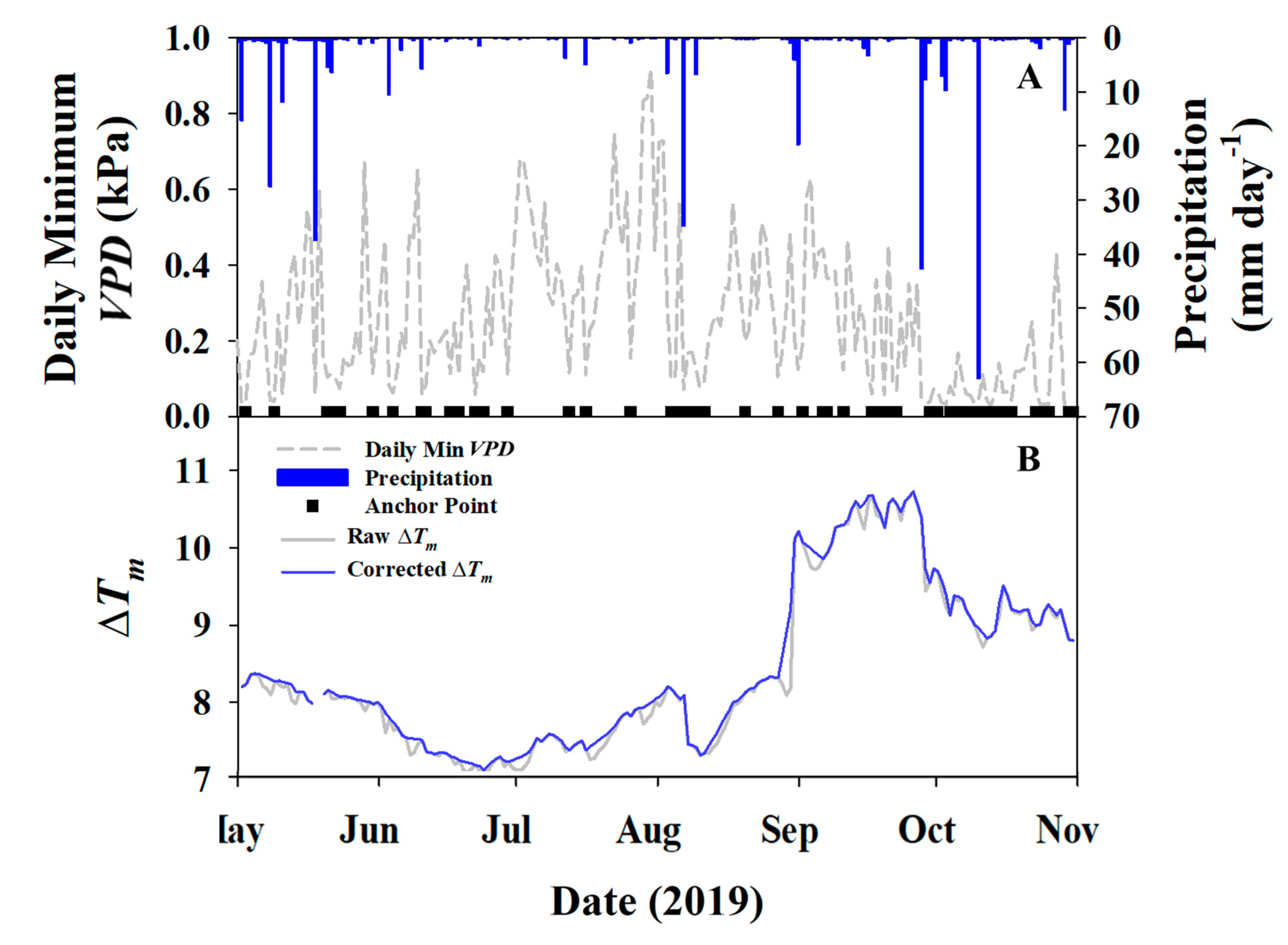
2.3.1. Baseline Corrections

It was determined after initial calculations of VPD and sap flow processing that nighttime flows were occurring at the site. VPD did not reach zero on a nightly basis, and there was not a consistent baseline for $\mathit{∆}{T}_m$ which introduces error into the original thermal dissipation equation. To account for this error and adjust $\mathit{∆}{T}_m$ for nighttime flows, a “baseline smoothing” process was utilized where daily minimum VPD was plotted with daily precipitation (Figure 1A) and days that had <0.1 kPa VPD and zero precipitation were considered days where calculated $\mathit{∆}{T}_m$ was accurate. The $\mathit{∆}{T}_m$ for remaining days were linearly gap-filled to create a smooth baseline. These new $\mathit{∆}{T}_m$ were then used to re-process the sap flow data.

2.3.2. Transpiration Scaling

Scaling up sap flow measurements to the footprint of the EC tower was done using surveys from trees in 29 individual 400 m² vegetation plots [23]. Within the 29 plots, there were 915 live individuals total for which the stem diameter and tree height were recorded. Using DBH, the basal area was then calculated for each individual tree, and an allometric equation was applied to calculate the sapwood area for each individual based on the basal area (y = 0.6075x + 0.0004, R² = 0.92). The total sapwood area per plot was divided by the total plot area to get sapwood area per unit ground area (m² m⁻²) for each plot, and a threshold value of 0.2 m² of sapwood area was used to differentiate between woodland and grassland plots (Figure S1). The average sapwood area per unit ground area for all of the woodland plots ($\overline{x}$ = 0.0012 m² m⁻² ± 0.0006, n = 19) was used to calculate the total sapwood area in the EC tower airshed. Transpiration (mm·day⁻¹) was then calculated by multiplying the average sap-flux density of all sap flow trees (kg m⁻² day⁻¹) by the average sapwood area per unit ground area. This bottom-up approach has been utilized in other studies [5,8] and validated by a review on methods for scaling up T measurements from tree to stand level [34]. It should be noted that this T estimate was based on oak allometry and sap flux, but there were other species present in the plots that may have different sapwood area to basal area ratios. Note that no understory species were included in this T estimate, including any woody vegetation with DBH < 0.5 cm.

2.4. Stable Isotopes

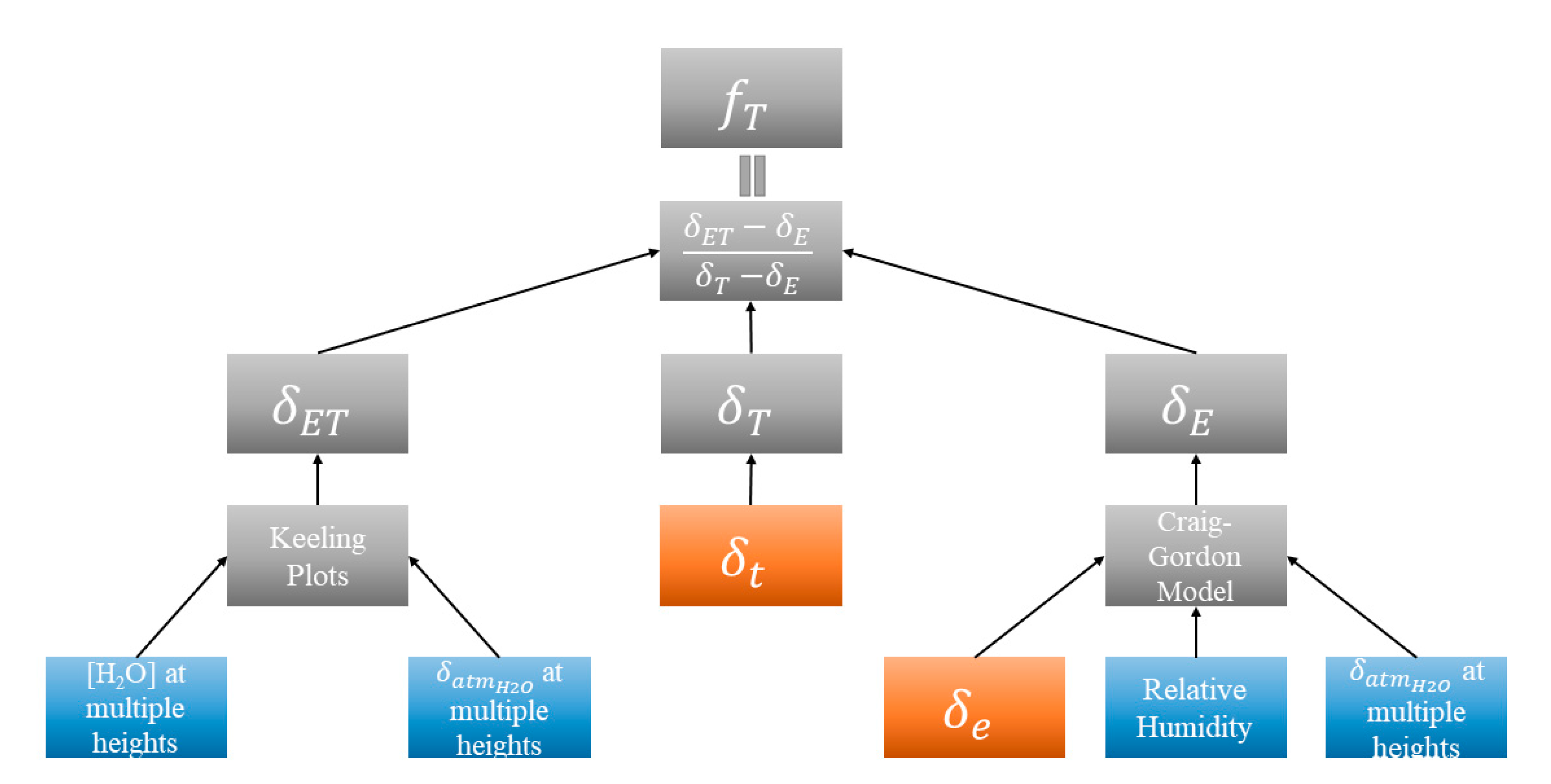
2.4.1. Method Framework

Given ET = E + T, the respective contributions of E and T to ET can be calculated using the isotopic mass balance approach, assuming a two-source model

$${\delta }_{ET}ET={\delta }_{E}E+{\delta }_{T}T$$

(1)

where ${\delta }_{ET}, {\delta }_E, \mathrm{and} {\delta }_T$ are equal to the isotopic composition of evapotranspiration, soil evaporation, and plant transpiration, respectively. The ratio of T to ET can then be calculated as

$$f_T=\frac{T}{ET}=\frac{{\delta }_{ET}-{\delta }_E}{{\delta }_T-{\delta }_E}$$

(2)

To use this method, the isotopic composition of water in three “end members” (i.e., soil, vegetation, and atmosphere) are needed, and the resulting ratios of each can be applied to total ET to get values of the individual components [35,36]. Differences in the isotopic composition of water in vegetation and in soil occur from fractionation during the evaporation process. The soil evaporating front changes with soil texture, soil moisture, and other environmental conditions, but is generally at the surface when the soil is saturated, and between 0.2–0.3 m in depth when the soil is not saturated [37,38,39]. Water is not fractionated during the transpiration process under steady-state conditions, so the isotopic composition of transpired water can be assumed equal to that of the xylem water [18,40,41]. Steady-state conditions are usually met around midday in field conditions [42]. Figure 2 shows the stepwise process for partitioning ET using the stable isotope method.

2.4.2. δ_ET, δ_E, and δ_T

The Keeling plot approach was used for obtaining δ_ET [35]. Measurements of the concentration and isotopic composition of water vapor at varying heights in the woodland canopy are sufficient to fit the linear model used in the Keeling plot approach [43,44,45]. Data for this approach were available from NEON [23]. Water vapor was collected by tubing at five different heights on a 30 min time step in the woodland canopy and circulated into the instrument hut where it was then analyzed for δ¹⁸O and δ²H via cavity ringdown spectroscopy (Picarro L2130-i, Picarro Inc., Santa Clara, CA, USA) in near-real-time. Water vapor concentrations at the same heights were included in the bundled EC data products. Only values from 10:30–14:00 h were used in the analysis.

Values of δ_E were attained from a combination of field samples and the Craig-Gordon Model (CGM) [46]

$${\delta }_E=\frac{{\delta }_e/{\alpha }^{*}-h{\delta }_v-{\epsilon }_{eq}-\left(1-h\right){\epsilon }_k}{\left(1-h\right)+\left(1-h\right){\epsilon }_k/1000}$$

(3)

where δ_e is the isotopic composition of liquid water at the soil evaporating front, α^* is the equilibrium fractionation factor (1.0098 and 1.084 at 20 °C for ¹⁸O and ²H, respectively [47]), h is relative humidity, δ_v is the isotopic composition of the background atmospheric water vapor, α_k is the isotopic fractionation factor (0.9755 and 0.9723 for ²H and ¹⁸O, respectively [48,49]), ε_eq is equal to 1000(1 − 1/α*), and ε_k is equal to 1000 (αk − 1).

Values for δ_T were attained directly through a sampling of twig water under steady-state assumptions, as has been done in other studies [35]. Under this scenario, it is assumed that the isotopic composition of the source water and transpired water are the same (${\delta }_X={\delta }_T$).

2.5. Field Sampling and Sample Analysis

2.5.1. Soil and Twig Sampling

To obtain isotopic values for soil water at the evaporating front (δ_e) and xylem water (δ_t), monthly soil and twig samples were taken. There was a total of nine sampling events during the study period that were carried out approximately every four weeks (Day of Year [DOY] 143, 170, 204, 234, 266, 294, 329, 351 in 2019 and DOY 24 in 2020). Soil samples (n = 4 per sampling day) were collected at midday (between 10:30–14:00 h) every month during the period of the study (May 2019–January 2020) to capture seasonal variability in δ_E. Samples were collected at 0.2 to 0.3 m depth when the soil was unsaturated, and taken from the surface when the soil was saturated. Soil saturation was determined at the site on sampling days before cores were taken. Samples were taken using a hand auger and immediately transferred into 12 mL glass vials and sealed with a cap and parafilm. To prevent evaporation, vials were transported upside down at ~34 °C to a freezer within 8 h. Samples were kept frozen until being processed at the Stable Isotopes for Biosphere Science (SIBS) Laboratory at Texas A&M University.

Twig samples (n = 4 per sampling day) were collected on the same days as soil samples during the same time window to satisfy steady-state conditions for xylem water sampling and to capture seasonal variability in δ_T. Samples were taken using a pole pruner from mature branches on trees containing sap flow sensors and were approximately three to five centimeters in length and less than 19 mm in diameter. The bark was then stripped from the twigs, and the twigs were immediately transferred into 12 mL glass vials and stored in the same manner as the soil samples.

2.5.2. Cryogenic Water Extractions and Analysis

All samples underwent water extractions using a cryogenic (liquid nitrogen) vacuum distillation system. Soil samples were extracted for approximately 75 min and twigs for approximately 55 min. The extracted water was then transferred to scintillation vials via pipet and stored at 34 °C until analysis.

The hydrogen and oxygen isotope analyses were performed using a Thermo Scientific High Temperature Conversion/Elemental Analyzer (TC/EA) coupled to a Conflo IV and a Thermo Scientific Delta V Advantage IRMS at the Stable Isotopes for Biosphere Science Laboratory, Texas A&M University. One micro liter (1 µL) of the sample was injected into TC/EA using a PAL autosampler. The injected sample was converted to H₂ and CO gas by pyrolysis reaction through a glassy carbon tube filled with glassy carbon chips and heated at 1370 °C. The H₂ and CO gas were separated by a 2 m packed gas chromatograph and were analyzed for the hydrogen and oxygen isotope ratios, respectively, in the Delta V Advantage IRMS. One sample was injected three times, and reported values are an average of these triplicate injections ± 0.01‰.

Calibration curves were derived using in-house water standards: SIBS-wA (δ²H = −390.8 ‰, δ¹⁸O = −50.10 ‰) and SIBS-wP (δ²H = −34.1 ‰, δ¹⁸O = −4.60 ‰). Quality control was performed using an in-house water standard, SIBS-wU (δ²H = −120.3 ‰, δ¹⁸O = −15.91 ‰). These in-house standards were calibrated using IAEA standards (VSMOW2, SLAP, and GISP) in 2009 and 2014.

2.6. f_T Analysis for Sampling Days

To determine how f_T compares between the stable isotope method and the residual of ET (ET_EC or ET₀) and T, only data from days when the soil and twig samples were collected (to provide surrogate values for the Keeling plots and CGM) were analyzed initially for the growing season (May–October 2019). Four methods were used to calculate f_T: (1) T/ET_EC, (2) T/ET₀, (3) δ²H-based stable isotope method, and (4) δ¹⁸O-based stable isotope method. This approach was used to provide insight as to how various partitioning methods compare to each other, how δ²H and δ¹⁸O compare within the stable isotope method, as well as how the various methods might change over time and with changes in seasonality. Samples were taken for November 2019 to January 2020 as well; however, it was assumed that f_T would be zero during this time, due to the trees having entered dormancy and the leaves abscising.

2.7. Predictive Model Development

An advantage of our study relative to others like it is the high data resolution and data availability across spatial and temporal scales that are collected by NEON. Due to the high-resolution data that is available throughout the growing season, two models were developed for predicting δ_e and δ_t for all days in the study period based on data from the sampling days. As obtaining soil and twig samples on a daily basis is cumbersome, expensive, and logistically infeasible, this inherently limits the utility of the stable isotope method by limiting the temporal resolution of surrogate values used in the CGM and Keeling plots. However, this barrier may be removed by predicting the isotopic composition of δ_e and δ_t (both δ²H and δ¹⁸O) based on other environmental variables that are easier to measure and do not require on-site presence.

Single and multiple linear regression models were tested using environmental data provided from NEON (air temperature, VPD, soil moisture, precipitation, soil heat flux, net radiation, water vapor concentration, water vapor isotopic composition, wind speed, and relative humidity) to predict the measured isotopic composition of δ_e and δ_t for sampling days during the growing season. Values from the δ_t predictive models were used directly for δ_T in the isotope method for partitioning ET, and values from the δ_e predictive models were used in the CGM to get δ_E. f_T was then determined every day from 11 May to 31 October for both δ²H and δ¹⁸O.

3. Results

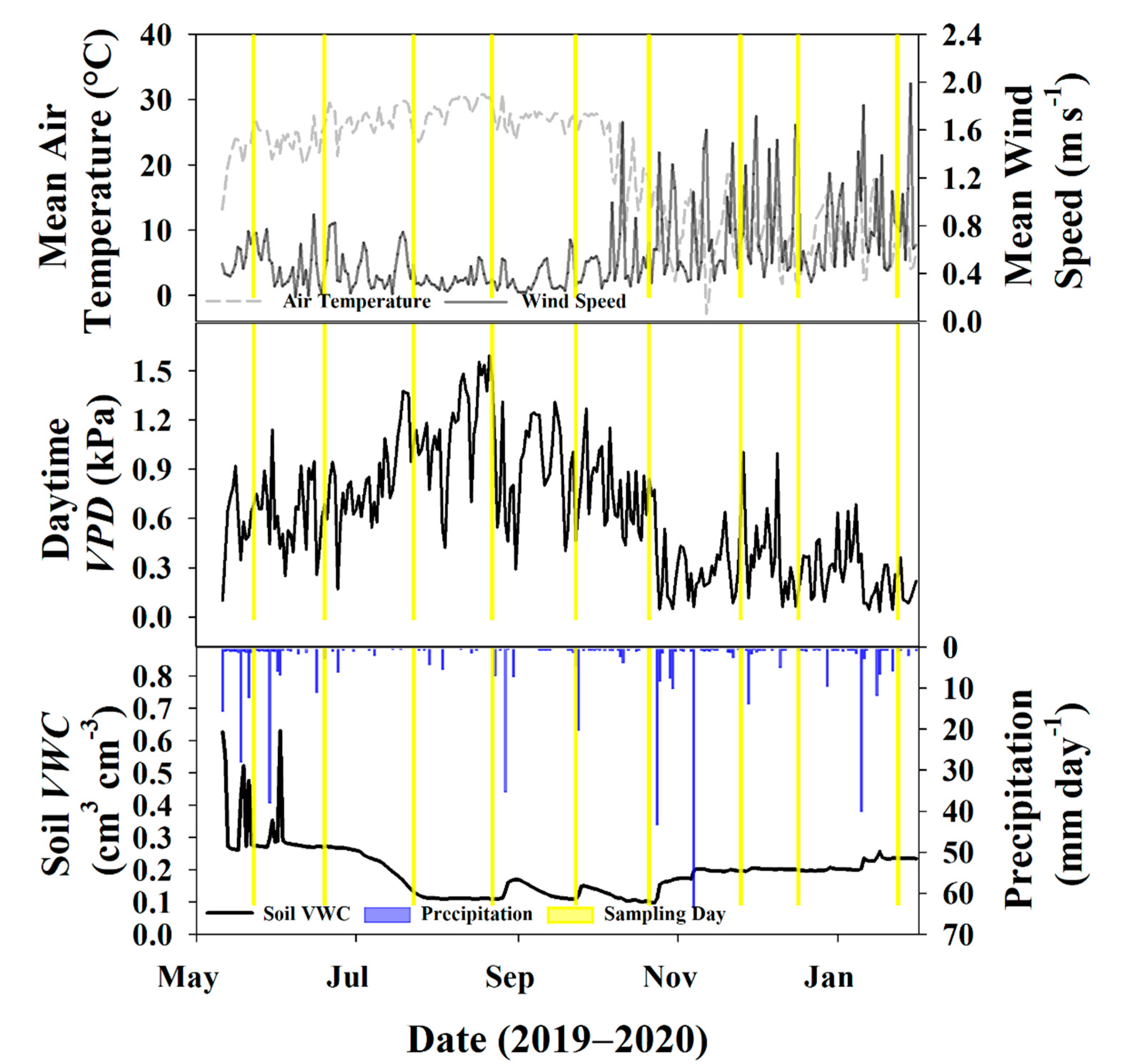
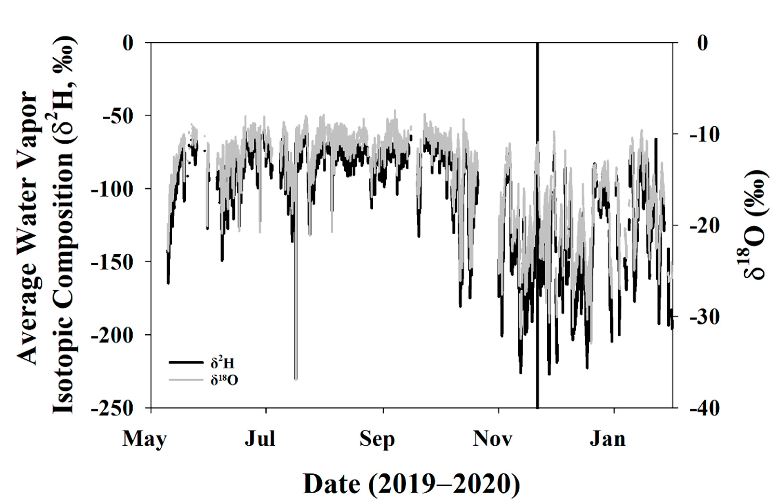
3.1. Environmental Data

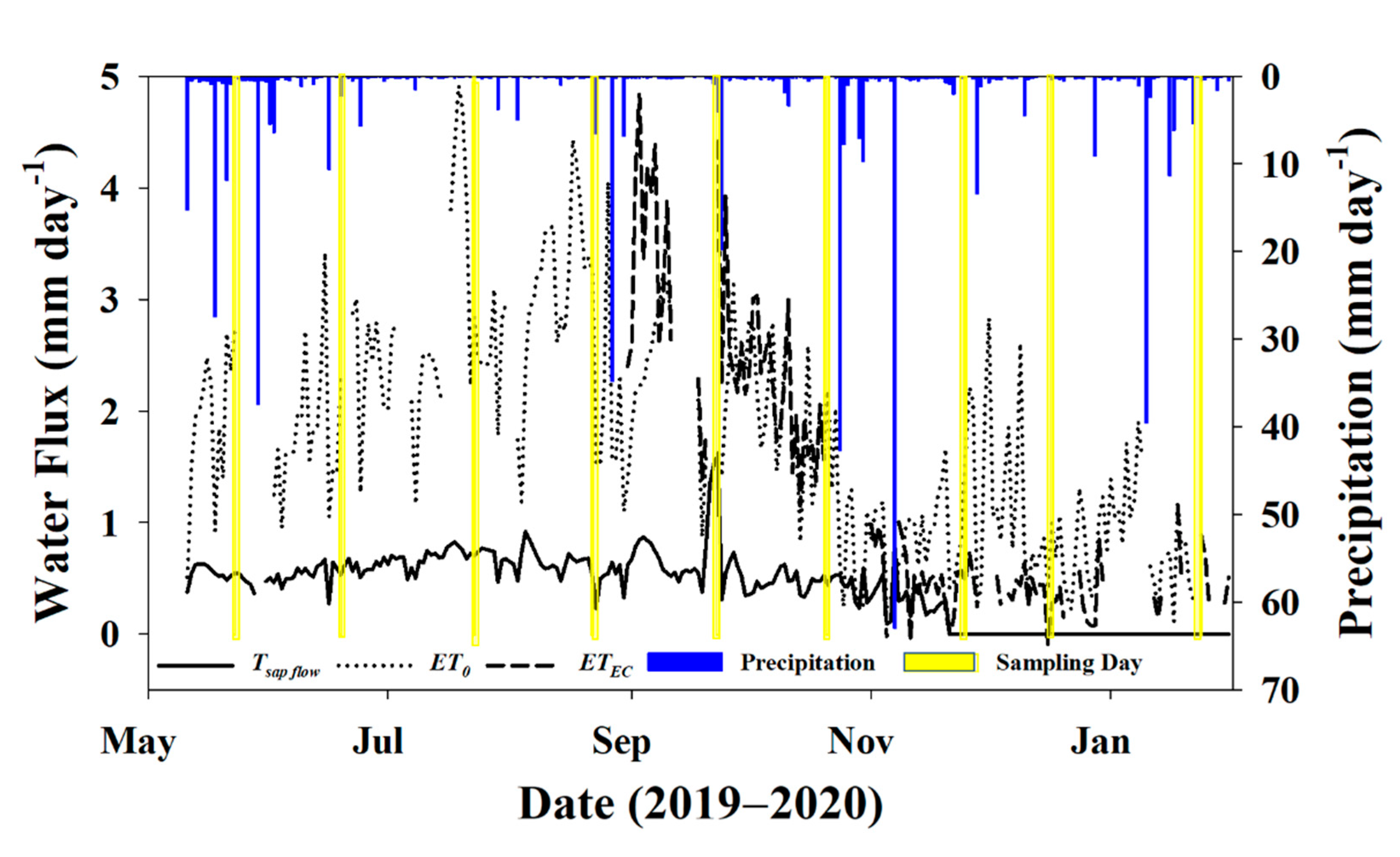
The majority of the growing season was characterized by high air temperature (>20 °C), stable wind speed, high daytime VPD (>0.3 kPa), and low soil moisture (<0.20 cm³ cm⁻³) following storms in May and June (Figure 3). Soil moisture fell consistently between July and September, and this same period experienced the highest daily air temperatures and the least amount of precipitation during the study period. Daytime VPD also reached its maxima in August, indicating peak summer conditions.

However, with the onset of the dormant season at the end of October and the beginning of November, the air temperature dropped markedly, and daily average wind speed showed higher fluctuations without the tree canopy acting as a buffer around the EC tower (Figure 3A). Due to changes with wind speed and air temperature dynamics, daytime VPD also began to drop, relative to growing season conditions (Figure 3B). The beginning of the dormant season was also characterized by a few large rain events that elevated soil moisture levels relative to the summer, and smaller, more frequent rain events maintained these higher levels throughout the end of the study (Figure 3C).

Water vapor isotopes also had distinct characteristics during the growing and dormant seasons. While trees were still transpiring, temperatures were still warm, and wind speeds were stable, average water vapor δ²H and δ¹⁸O was also relatively stable (Figure 4). As trees began to senesce in October and November, resulting in less stomatal conductance, the boundary layer conditions changed, and this is reflected in the higher degree of fluctuations of water vapor isotopes in the dormant season relative to the growing season.

3.2. Water Fluxes

Due to technical issues, actual evapotranspiration (ET_EC) was unreliable for the beginning of the study period (Figure 5). However, there was a moderate agreement for daily evapotranspiration estimated by Penman–Monteith (ET₀) and the eddy covariance method for the remainder of the growing season (2.25 ± 0.89 mm·day⁻¹ and 2.60 ± 0.92 mm·day⁻¹, respectively). The eddy covariance method provided sufficient data 40% of the time from 11 May 2019 to 31 January 2020 (107/265 days in the study period), and ET₀ provided sufficient data 88% of the time (233/265 days).

Total precipitation during the measurement period prior to dormancy (11 May to 31 October 2019) was 315.77 mm, or about 38% of MAP, which was 36% below normal for that time of year based on data from the last 50 years [50]. Total T, ET₀, and ET_EC for this same time period were 102.2 mm (12% of MAP), 391.5 mm (47% of MAP), and 452.4 mm (54% of MAP), respectively, for that partial growing season. Average transpiration for the study period was 0.59 ± 0.18 mm·day⁻¹, and trees were officially deemed dormant on DOY 325 (21 November 2019) based on sap flow data, just before the November sampling event. The average ET₀ and ET_EC for the dormant season (November–January) was 0.94 ± 0.55 and 0.44 ± 0.28 mm·day⁻¹.

3.3. Sampling Days

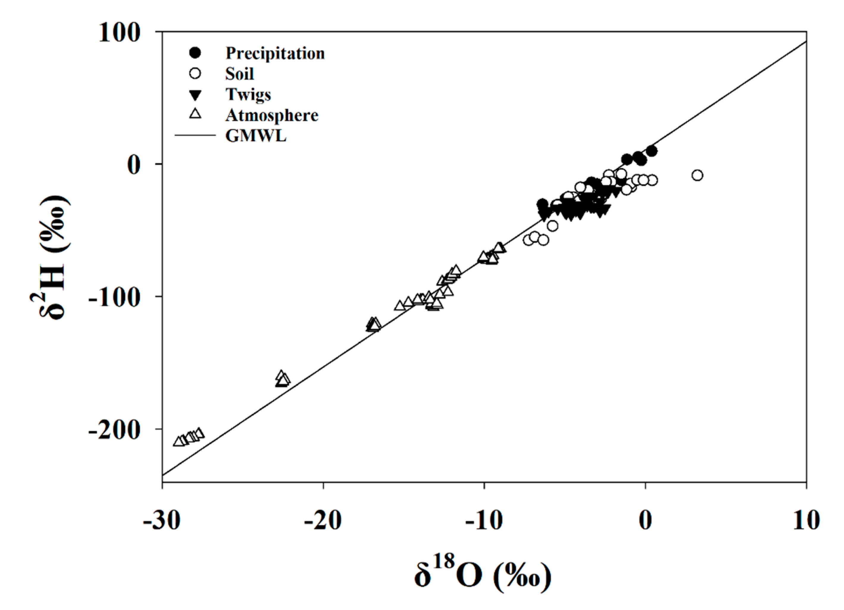
3.3.1. Global Meteoric Water Line and Keeling Plot

The isotopic composition (δ¹⁸O and δ²H) of atmospheric and precipitation samples fell closely along the global meteoric water line (GMWL), as was expected (Figure 6). The soil samples fell to the right of the GMWL, indicating preferential evaporation of lighter isotopologues of water and soil enrichment with the heavier isotopologues. These results indicate the evaporative fractionation of soil water and an appropriate degree of separation between the signals of twig and soil water isotope ratios.

The average of the inverse water concentration between 10:30–14:00 h was used against the isotope ratio (both δ¹⁸O and δ²H) during the same time period to construct turbulent mixing relationships, or Keeling plots. In examining Keeling Plot relationships, we found that the inverse water vapor concentration was closely related to isotopic ratios during all sampling events (p < 0.05) except July (δ²H and δ¹⁸O) and October (δ¹⁸O) with R² ranging up to 0.86 (

Table 1. Descriptive statistics for linear regression (Keeling Plot) analyses for sampling events during the growing season. Sample size (N) is the total of water vapor data from 10:30 to 14:00 at five different heights in the forest canopy for each sampling day. DOY, Day of Year.

Sampling DOY 2019	Stable Isotope	Keeling Plot
		N	Slope	δET	R2	p-Value
143	δ18O	21	−236.37	−1.07	0.71	<0.001
	δ2H	21	−1853.90	−3.37	0.77	<0.001
170	δ18O	29	−97.11	−7.86	0.61	<0.001
	δ2H	29	−864.74	−47.32	0.86	<0.001
204	δ18O	29	109.86	−19.60	0.09	0.11
	δ2H	29	184.18	−112.54	0.02	0.52
234	δ18O	29	103.95	−13.95	0.13	0.05
	δ2H	29	−682.05	−44.91	0.57	<0.001
266	δ18O	16	−368.38	3.03	0.44	0.005
	δ2H	16	−1084.78	−28.37	0.29	0.03
294	δ18O	28	7.11	−13.57	0.03	0.4
	δ2H	28	−331.99	−76.86	0.72	<0.001

). As 1/[H₂O] increased, heavier isotopes tended to decrease. The monthly predictions of δ_ET from Keeling plots varied widely throughout the study period for both H and O.

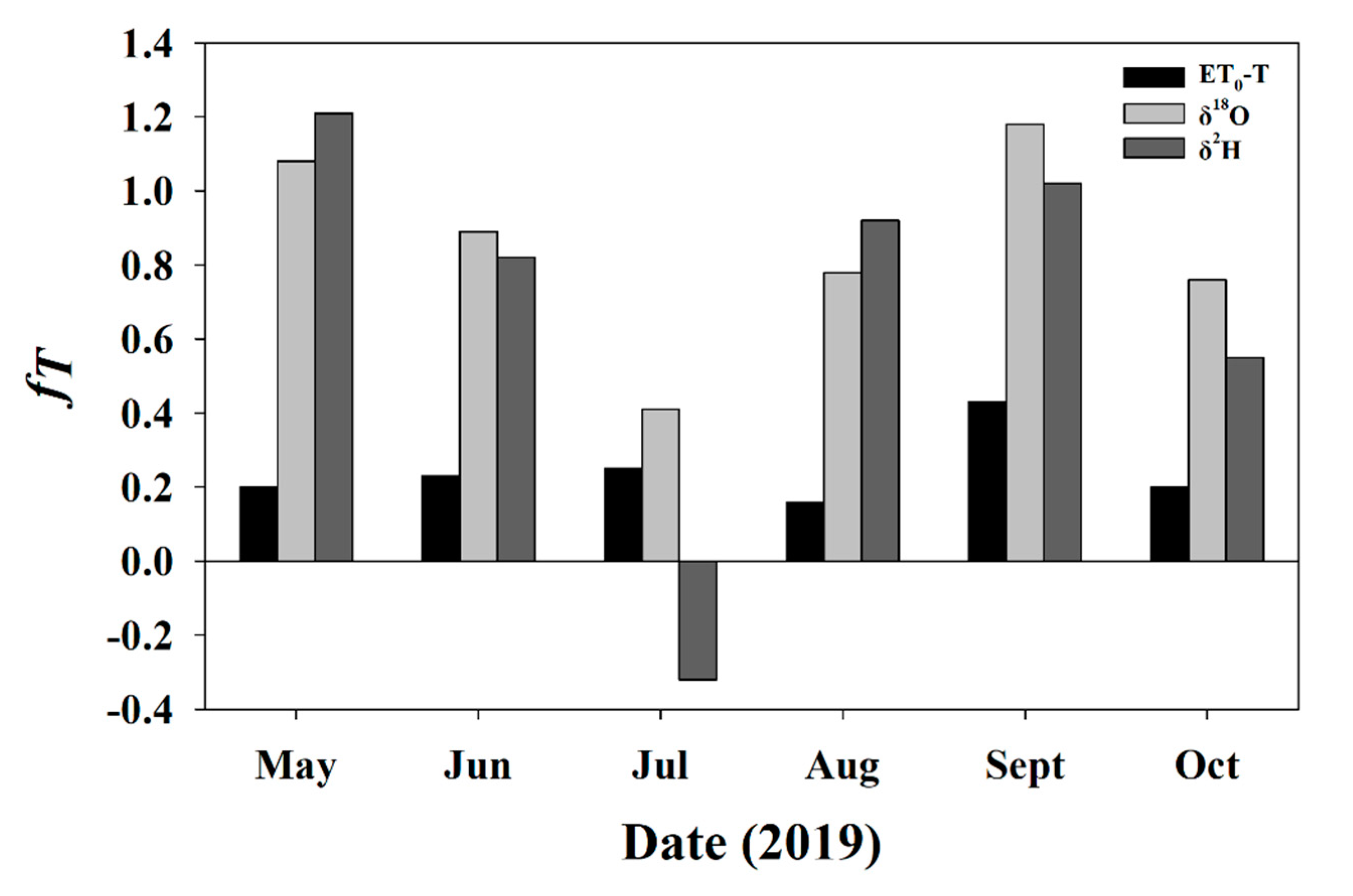
3.3.2. f_T for Soil and Twig Sampling Days

The average f_T calculated from the stable isotope method with data from only sampling days was 0.85 ± 0.27 for δ¹⁸O and 0.7 ± 0.55 for δ²H. On two of the sampling days where the Keeling Plots had significant slopes (May and September) f_T exceeded 100% of total ET for both δ²H and δ¹⁸O. Additionally, the δ²H July sampling event had a f_T < 0, though the Keeling Plot for this event was not significant. The average f_T calculated from ET₀ was substantially lower (0.25 ± 0.1) and never went below 0 or above 1 (Figure 7).

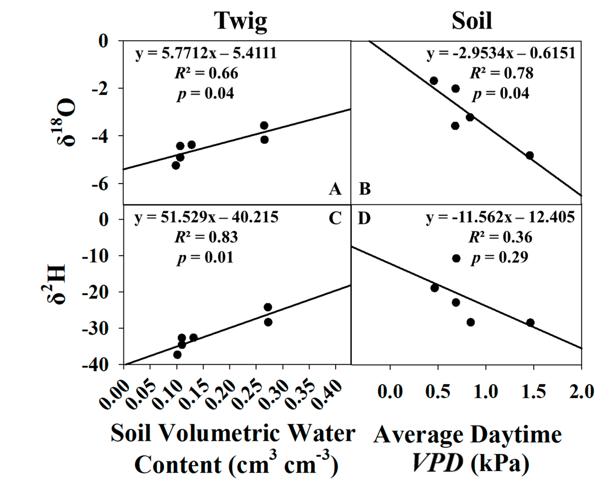
3.4. Predictive Models for Growing Season and Dormant Season Sampling Days

It was determined that average daytime VPD (between 6:00–18:00 h) and average soil moisture at 0.16 m depth were the single best predictors of δ_e and δ_t, respectively (Figure 8). Soil moisture at other depths was tested; however, 0.16 m performed the best and was empirically logical as it is the depth in-between saturated (surface) and unsaturated (0.2 to 0.3 m) sample depths. Equations from Figure 8 were then used to estimate daily values of δ_e and δ_t for use in the stable isotope method to partition ET. All growing season models were significant at the 95% confidence level, with the exception of the δ_e δ²H model. A total of 6 data points were used in the δ_t models, but the July sampling event was excluded from the δ_e models as its Keeling Plot had an insignificant slope (Table 1), and its isotope ratio values were outliers compared to the other five months.

For the dormant season, the same approach was utilized for δ_e and δ_t modeling during the growing season. The additional data from November 2019–January 2020 was added to the four models, and new regressions were conducted. The δ_t models were mostly unaffected and continued to be significant for both δ²H and δ¹⁸O (Figure 9). However, for the δ_e models, the slope of the regression line switched directions, the R² values dropped markedly, and the p-value for the previously significant δ_e δ¹⁸O model jumped to 0.75. Due to these reasons, δ_e and δ_t were not modeled for the dormant season.

3.5. Entire Growing Season

3.5.1. Keeling Plot

To predict δ_ET for the entire growing season, atmospheric isotope data and water vapor concentration data for every day from 11 May 2019 to 31 October 2019 were collected and filtered for data only during 10:30–14:00 for each of the five heights in EC tower. This data was then input into Rstudio and underwent linear regression (Keeling plots/turbulent mixing relationships) for every day there were sufficient data, for both δ¹⁸O and δ²H. Relevant parameters were extracted for each day, including sample size (N), slope, intercept (δ_ET), R², and a p-value, which are reported in Table S3. Of the 164 days in the growing season, there were sufficient EC tower data to construct Keeling plots for 131 days (80%). Of these 131 days with complete data, there were significant slopes for 112 days (86%) using δ²H, and 89 days (68%) using δ¹⁸O. Keeling plots were not constructed for the dormant season, due to issues with δ_e modeling and unstable boundary layer conditions.

3.5.2. Craig-Gordon Model

Of the 164 days in the growing season, the CGM successfully ran for 148 (90%) of days. In this case, δ¹⁸O and δ²H performed equivalently in terms of producing values for δ_E, and the limiting factor for running the CGM was obtaining complete water vapor isotope data from the EC tower and CRDS. Sixteen days (10%) were missing or had incomplete water vapor isotope data. Relative humidity data were complete for the entire season, as well as soil moisture used to predict δ_e.

3.5.3. Daily f_T for Entire Study Period

Days with insignificant Keeling plots (p-value > 0.05) were excluded for f_T using the stable isotope method, along with days having an f_T < 0 or >1.0 for all methods. Day 131 was excluded, due to site setup and disturbance. For the first approach (T/ET_EC), the average f_T was 0.36 ± 0.31, and there was a total of 70 days (43%) with valid and complete data. For the second approach (T/ET₀), the average f_T was 0.28 ± 0.11, and there was a total of 140 days (86%) with valid and complete data. Both δ²H and δ¹⁸O had an average f_T of 0.77 ± 0.20, though there were only valid data for 79 and 56 of the 164 days (48% and 34%), respectively. The results from raw calculated f_T are reported in Figure 10.

On average, f_T calculated from T/ET_EC or T/ET₀ were 41% and 49% lower than those calculated from the stable isotope method. Minimum f_T calculated from the stable isotope method was nearly always greater than the maximum value calculated by traditional methods (T/ET_EC, T/ET₀). To remove this potential systematic bias from the estimates, f_T from the stable isotope method was bias-corrected to ET₀ (Figure 11 left) and ET_EC (Figure 11 right) using the average difference as the trends (direction and slope) were similar, despite the absolute magnitude being different. The average ET₀ bias-corrected stable isotope f_T was 0.40 ± 0.15, and the ET_EC bias-corrected f_T was 0.32 ± 0.15, which are only 4–12% greater than traditional f_T, as opposed to 41–49% before normalization.

4. Discussion

This study demonstrated the utility of using a combination of stable isotopes, sap flux, and eddy covariance techniques to partition ET in an oak woodland and introduces a novel methodology using CRDS water vapor isotopes. The stable isotope technique has benefited from improved technological advancements with cavity ringdown spectroscopy and high-temporal resolution vapor collection systems that work in unison with eddy covariance and sap flux systems. However, the stable isotope method for partitioning ET did not compare favorably with more traditional techniques, such as using the difference of total ET from eddy covariance or ET₀ along with T estimated from sap flow measurements, on any sampling day. There was a 41–49% overestimation of f_T in this system when utilizing the stable isotope technique compared to ET_EC or ET₀ relative to sap-flux-based T. When using the average difference to normalize f_T for either δ¹⁸O or δ²H the overestimation was reduced to 4–12%, which is within the range found from other studies [10]. This suggests that there may be a systematic bias to the CGM, which leads to the overestimation of f_T in natural systems, and this bias should be investigated thoroughly in the future.

When comparing δ¹⁸O and δ²H within the stable isotope method, there was much agreement between the two, which contrasts with results and conclusions from other studies [10,21,32]. Typically, δ²H is utilized over δ¹⁸O, due to its higher degree of sensitivity. However, the high temporal-resolution data provided by the CRDS was able to provide the necessary data resolution for δ¹⁸O to have a similar performance to δ²H. Both δ¹⁸O and δ²H were able to satisfy requirements for the CGM 90% of the time, and δ¹⁸O only slightly underperformed in the Keeling Plot approach when compared to δ²H (68% and 86% of the study period). This may be in part to the more sensitive fractionation coefficient for δ²H relative to δ¹⁸O, which increases the potential for significant results, or there may have been evaporation in soil and twig sample vials during transit from the field to the lab (for IRMS analysis), which could have led to the error. However, these results complement those from the GMWL, indicating that the stable isotope approach can successfully be utilized within the framework provided in this study. The limiting factors in constructing Keeling plots at the daily scale using the CRDS and the EC tower are having a robust data collection system and a field crew that can maintain and repair the instruments in the case of malfunction or failure. While δ²H slightly outperformed δ¹⁸O, which was expected, δ¹⁸O performed more strongly than previous studies have suggested. This indicates that the high temporal-resolution data collected by the CRDS is truly necessary to make this approach viable at the daily scale for both stable isotopes of water.

A severe limiting factor to the utility of the stable isotope approach for partitioning ET, however, is the ability to obtain soil and xylem water samples from the field at fine enough resolutions to examine multi-day or seasonal trends in δ_e and δ_t. For this study, field samples were only feasibly obtained monthly, which limited the data available for partitioning initially to one day per month. However, due to partnership with NEON, a diverse suite of data was available at a much higher resolution, and soil and xylem water were successfully modeled using 30 min VPD and soil moisture data, respectively. This enabled us to partition ET from what was initially only six sampling events, to 79 and 56 days for δ²H and δ¹⁸O, respectively. While this was still only 56% and 48% of all days in the growing season, the stable isotope method was markedly improved by utilizing a combination of modeling and field sampling events. Our model also coincides with results from recent work that established tree water status, driven by soil water potential and atmospheric conditions, was the main reason for source water partitioning and isotopic fractionation during a 7-week lysimeter experiment in Switzerland [51].

While 0.16 m soil depth worked best during the growing season for this study, other depths may work better under different precipitation regimes. For instance, if the soil constantly remained unsaturated during the growing season, then 0.2 to 0.3 m may be more appropriate to model δ_e dynamics. Similarly, under flooded conditions, it would be more appropriate to model δ_e from soil moisture at the surface. While source water for trees was not independently identified during this study, that may be advantageous in the future to verify the assumption that δ_X = δ_T. Furthermore, modeled δ_t in this study was based solely on xylem water from Quercus spp. twig samples. However, these values may change if other species in the tower footprint were sampled instead. A more accurate estimation of both T and δ_t may be achieved by measuring sap flow in additional species and sampling those species for xylem water simultaneously. Steady-state assumptions were justified in this study, due to sampling in the mid-day and afternoon conditions, but there is an increasing body of evidence that in the early morning and evening, steady-state conditions are no longer present. This should be taken into consideration for future work; however, some studies have also shown that f_T calculated both ways is similar at the end of the day [36].

When dormant season data was added to the δ_e and δ_t models, δ_t remained significant as the water inside of the trees were not being utilized during dormancy; however, the δ_e models became unreliable. This suggests that evaporation dynamics during the dormant season are different than during the growing season, and that these dynamics were not successfully captured in the CGM. Furthermore, atmospheric water vapor isotopes at the onset of and during the dormant season are considerably more variable than during the growing season. This is likely due to the physical barrier that leaves give at the top of the canopy, as well as the regulating properties of active transpiration on the boundary layer micrometeorology [52].

It should be noted that forests and woodlands inherently have more variability and heterogeneity when compared to engineered or agricultural systems like croplands, and this may result, in part, account for variance observed in the boundary layer. However, the combination of insignificant δ_e models and sporadic water vapor concentrations just before and after trees lose their leaves suggests that the CGM cannot be utilized during the dormant season in such systems.

While the application of δ_e and δ_t modeling may be used to interpolate between sampling events during the growing season, the utility of the approach is severely limited during the dormant season, due to shifts in boundary layer conditions and evaporation dynamics at the soil surface. Additional experiments with the CGM using high temporal-resolution data collection systems similar to this study are warranted to reconcile discrepancies for CGM performance over changes in seasonality. While in this study, the assumption that T was negligible during the dormant season may be appropriate, this may not be the case in other systems.

5. Conclusions

This study demonstrated a novel methodology for partitioning ET using a combination of the high-resolution stable isotope, sap flux, and eddy covariance techniques over multiple seasons in a natural oak woodland site. To the best of our knowledge, this is the first report of utilizing a CRDS for ET partitioning at this timescale and under these conditions, and only the second report of direct partitioning comparisons between stable isotope derived f_T and f_T from sap flow and eddy covariance. Furthermore, we have developed predictive models for estimating the isotopic composition of the soil (δ_e) and xylem (δ_t) water (both components necessary for the stable isotope-based ET partitioning method) on days when field samples cannot be taken, by utilizing common environmental and micrometeorological data. With the high-frequency data made available through NEON, we found that δ²H and δ¹⁸O produced similar results, where, in the literature, δ²H is typically only utilized. The utility of the stable isotope method for partitioning ET has been markedly improved with the with the integration of high-temporal resolution data collection systems, such as an EC tower coupled with a CRDS, along with field sampling of soil and twigs. However, further refinement of the methodology, particularly in natural systems, is still needed to reconcile potential biases inherent in this approach, and to test the utility of the proposed δ_e and δ_t models under wide-ranging conditions. We recommend that future investigations continue to refine the use of high frequency stable isotope data for novel application in partitioning ET, given the advantages of a single integrated whole-canopy estimation.

References

1. Trenberth Kevin, E.; Smith, L.; Qian, T.; Dai, A.; Fasullo, J. Estimates of the Global Water Budget and Its Annual Cycle Using Observational and Model Data. J. Hydrometeorol. 2007, 8, 758. [Google Scholar] [CrossRef]
2. Wilcox, B.; Breshears, D.; Seyfried, M. Water Balance on Rangelands. Encycl. Water Sci. 2003, 791–794. [Google Scholar] [CrossRef]
3. Good, S.P.; Moore, G.W.; Miralles, D.G. A mesic maximum in biological water use demarcates biome sensitivity to aridity shifts. Nat. Ecol. Evol. 2017, 1, 1883–1888. [Google Scholar] [CrossRef]
4. Helman, D.; Lensky, I.M.; Osem, Y.; Rohatyn, S.; Rotenberg, E.; Yakir, D. A biophysical approach using water deficit factor for daily estimations of evapotranspiration and CO2 uptake in Mediterranean environments. Biogeosciences 2017, 14, 3909–3926. [Google Scholar] [CrossRef] [Green Version]
5. Ford, C.R.; Hubbard, R.M.; Kloeppel, B.D.; Vose, J.M. A comparison of sap flux-based evapotranspiration estimates with catchment-scale water balance. Agric. For. Meteorol. 2007, 145, 176–185. [Google Scholar] [CrossRef]
6. Shi, T.T.; Guan, D.X.; Wu, J.B.; Wang, A.Z.; Jin, C.J.; Han, S.J. Comparison of methods for estimating evapotranspiration rate of dry forest canopy: Eddy covariance, Bowen ratio energy balance, and Penman-Monteith equation. J. Geophys. Res. Atmos. 2008, 113, 15. [Google Scholar] [CrossRef]
7. Tie, Q.; Hu, H.; Tian, F.; Holbrook, N.M. Comparing different methods for determining forest evapotranspiration and its components at multiple temporal scales. Sci. Total Environ. 2018, 633, 12–29. [Google Scholar] [CrossRef] [PubMed]
8. Williams, D.G.; Cable, W.; Hultine, K.; Hoedjes, J.C.B.; Yepez, E.A.; Simonneaux, V.; Er-Raki, S.; Boulet, G.; de Bruin, H.A.R.; Chehbouni, A.; et al. Evapotranspiration components determined by stable isotope, sap flow and eddy covariance techniques. Agric. For. Meteorol. 2004, 125, 241–258. [Google Scholar] [CrossRef]
9. Kool, D.; Agam, N.; Lazarovitch, N.; Heitman, J.L.; Sauer, T.J.; Ben-Gal, A. A review of approaches for evapotranspiration partitioning. Agric. For. Meteorol. 2014, 184, 56–70. [Google Scholar] [CrossRef]
10. Aouade, G.; Ezzahar, J.; Amenzou, N.; Er-Raki, S.; Benkaddour, A.; Khabba, S.; Jarlan, L. Combining stable isotopes, Eddy Covariance system and meteorological measurements for partitioning evapotranspiration, of winter wheat, into soil evaporation and plant transpiration in a semi-arid region. Agric. Water Manag. 2016, 177, 181–192. [Google Scholar] [CrossRef]
11. Xu, Z.; Yang, H.; Liu, F.; An, S.; Cui, J.; Wang, Z.; Liu, S. Partitioning evapotranspiration flux components in a subalpine shrubland based on stable isotopic measurements. Bot. Stud. 2008, 49, 351–361. [Google Scholar]
12. Wilson, K.B.; Hanson, P.J.; Mulholland, P.J.; Baldocchi, D.D.; Wullschleger, S.D. A comparison of methods for determining forest evapotranspiration and its components: Sap-flow, soil water budget, eddy covariance and catchment water balance. Agric. For. Meteorol. 2001, 106, 153–168. [Google Scholar] [CrossRef]
13. Moore, G.W.; Cleverly, J.R.; Owens, M.K. Nocturnal transpiration in riparian Tamarix thickets authenticated by sap flux, eddy covariance and leaf gas exchange measurements. Tree Physiol. 2008, 28, 521–528. [Google Scholar] [CrossRef] [Green Version]
14. Granier, A. Evaluation of transpiration in a Douglas-fir stand by means of sap flow measurements. Tree Physiol. 1987, 3, 309–320. [Google Scholar] [CrossRef] [PubMed]
15. Granier, A. Une nouvelle méthode pour la mesure du flux de sève brute dans le tronc des arbres. Ann. Sci. 1985, 42, 193–200. [Google Scholar] [CrossRef]
16. Nier, A. The development of A high-resolution mass-spectrometer—A reminiscence. J. Am. Soc. Mass Spectrom. 1991, 2, 447–452. [Google Scholar] [CrossRef] [Green Version]
17. Walker, C.D.; Brunel, J.P. Examining evapotranspiration in a semi-arid region using stable isotopes of hydrogen and oxygen. J. Hydrol. 1990, 118, 55–75. [Google Scholar] [CrossRef]
18. Brunel, J.-P.; Walker, G.R.; Kennett-Smith, A.K. Field validation of isotopic procedures for determining sources of water used by plants in a semi-arid environment. J. Hydrol. 1995, 167, 351–368. [Google Scholar] [CrossRef]
19. Brunel, J.P.; Walker, G.R.; Dighton, J.C.; Monteny, B. Use of stable isotopes of water to determine the origin of water used by the vegetation and to partition evapotranspiration. A case study from HAPEX-Sahel. J. Hydrol. 1997, 188, 466–481. [Google Scholar] [CrossRef]
20. Munksgaard, N.C.; Wurster, C.M.; Bird, M.I. Continuous analysis of δ18O and δD values of water by diffusion sampling cavity ring-down spectrometry: A novel sampling device for unattended field monitoring of precipitation, ground and surface waters. Rapid Commun. Mass Spectrom. 2011, 25, 3706–3712. [Google Scholar] [CrossRef] [PubMed]
21. Wei, Z.; Yoshimura, K.; Okazaki, A.; Kim, W.; Liu, Z.; Yokoi, M. Partitioning of evapotranspiration using high-frequency water vapor isotopic measurement over a rice paddy field. Water Resour. Res. 2015, 51, 3716–3729. [Google Scholar] [CrossRef]
22. Soil Survey Staff, NRCS. Web Soil Survey; United States Department of Agriculture: Washington, DC, USA, 2019.
23. NEON. National Ecological Observatory Network; Battelle: Boulder, CO, USA, 2020. [Google Scholar]
24. Michael, W.; Jan, H. Biohydrologic effects of eastern redcedar encroachment into grassland, Oklahoma, USA. Biologia 2013, 68, 1132–1135. [Google Scholar] [CrossRef]
25. Jones, H.G. Plants and Microclimate: A Quantitative Approach to Environmental Plant Physiology; Cambridge University Press: Cambridge, UK, 1992; p. 428. [Google Scholar]
26. Kljun, N.; Calanca, P.; Rotach, M.W.; Schmid, H.P. A simple two-dimensional parameterisation for Flux Footprint Prediction (FFP). Geosci. Model Dev. 2015, 8, 3695–3713. [Google Scholar] [CrossRef] [Green Version]
27. Venkatram, A. Estimating the Monin-Obukhov length in the stable boundary layer for dispersion calculations. Bound. Layer Meteorol. 1980, 19, 481–485. [Google Scholar] [CrossRef]
28. Zotarelli, L.; Dukes, M.D.; Romero, C.C.; Migliaccio, K.W.; Morgan, K.T. Step by Step Calculation of the Penman-Monteith Evapotranspiration (FAO-56 Method); Institute of Food and Agricultural Sciences. University of Florida: Gainesville, FL, USA, 2018. [Google Scholar]
29. Moore, G.W.; Bond, B.J.; Jones, J.A.; Phillips, N.; Meinzer, F.C. Structural and compositional controls on transpiration in 40-and 450-year-old riparian forests in western Oregon, USA. Tree Physiol. 2004, 24, 481–491. [Google Scholar] [CrossRef] [PubMed] [Green Version]
30. Vertessy, R.A.; Watson, F.G.R.; O′Sullivan, S.K. Factors determining relations between stand age and catchment water balance in mountain ash forests. For. Ecol. Manag. 2001, 143, 13–26. [Google Scholar] [CrossRef]
31. McDowell, N.; Barnard, H.; Bond, B.J.; Hinckley, T.; Hubbard, R.M.; Ishii, H.; Köstner, B.; Magnani, F.; Marshall, J.D.; Meinzer, F.C.; et al. Relatsh between Tree Height Leaf Area: Sapwood Area Ratio. Oecologia 2002, 132, 12. [Google Scholar] [CrossRef]
32. Gebauer, T.; Horna, V.; Leuschner, C. Variability in radial sap flux density patterns and sapwood area among seven co-occurring temperate broad-leaved tree species. Tree Physiol. 2008, 28, 1821–1830. [Google Scholar] [CrossRef] [Green Version]
33. Clearwater, M.J.; Goldstein, G.; Holbrook, N.M.; Meinzer, F.C.; Andrade, J.L. Potential errors in measurement of nonuniform sap flow using heat dissipation probes. Tree Physiol. 1999, 19, 681–687. [Google Scholar] [CrossRef] [Green Version]
34. Mackay, D.S.; Ewers, B.E.; Loranty, M.M.; Kruger, E.L. On the representativeness of plot size and location for scaling transpiration from trees to a stand. J. Geophys. Res. Biogeosci. 2010, 115, 14. [Google Scholar] [CrossRef] [Green Version]
35. Xiao, W.; Wei, Z.; Wen, X. Evapotranspiration partitioning at the ecosystem scale using the stable isotope method—A review. Agric. For. Meteorol. 2018, 263, 346–361. [Google Scholar] [CrossRef]
36. Zhang, S.; Wen, X.; Wang, J.; Yu, G.; Sun, X. The use of stable isotopes to partition evapotranspiration fluxes into evaporation and transpiration. Acta Ecol. Sin. 2010, 30, 201–209. [Google Scholar] [CrossRef]
37. Barnes, C.J.; Allison, G.B. Tracing of water movement in the unsaturated zone using stable isotopes of hydrogen and oxygen. J. Hydrol. 1988, 100, 143–176. [Google Scholar] [CrossRef]
38. Sprenger, M.; Leistert, H.; Gimbel, K.; Weiler, M. Illuminating hydrological processes at the soil-vegetation-atmosphere interface with water stable isotopes. Rev. Geophys. 2016, 54, 674–704. [Google Scholar] [CrossRef] [Green Version]
39. Zimmermann, U.; Ehhalt, D.; Muennich, K.O. Soil-Water Movement and Evapotranspiration: Changes in the Isotopic Composition of the Water; International Atomic Energy Agency: Vienna, Austria, 1967. [Google Scholar]
40. Ehleringer, J.R.; Dawson, T.E. Water uptake by plants: Perspectives from stable isotope composition. Plant Cell Environ. 1992, 15, 1073–1082. [Google Scholar] [CrossRef]
41. Yepez, E.A.; Williams, D.G.; Scott, R.L.; Lin, G. Partitioning overstory and understory evapotranspiration in a semiarid savanna woodland from the isotopic composition of water vapor. Agric. For. Meteorol. 2003, 119, 53–68. [Google Scholar] [CrossRef]
42. Flanagan, L.B.; Comstock, J.P.; Ehleringer, J.R. Comparison of Modeled and Observed Environmental Influences on the Stable Oxygen and Hydrogen Isotope Composition of Leaf Water in Phaseolus vulgaris L. Plant Physiol. 1991, 96, 588. [Google Scholar] [CrossRef] [Green Version]
43. Keeling, C.D. The concentration and isotopic abundances of atmospheric carbon dioxide in rural areas. Geochim. Cosmochim. Acta 1958, 13, 322–334. [Google Scholar] [CrossRef]
44. Keeling, C.D. The concentration and isotopic abundances of carbon dioxide in rural and marine air. Geochim. Cosmochim. Acta 1961, 24, 277–298. [Google Scholar] [CrossRef]
45. Yakir, D.; Sternberg, L.d.S.L. The use of stable isotopes to study ecosystem gas exchange. Oecologia 2000, 123, 297–311. [Google Scholar] [CrossRef] [PubMed]
46. Craig, H.; Gordon, L.I. Deuterium and oxygen 18 variations in the ocean and the marine atmosphere. In Proceedings of the Conference on Stable Isotopes in Oceanographic Studies and Paleotemperatures, Spoleto, Italy, 26–30 July 1965; pp. 9–130. [Google Scholar]
47. Majoube, M. Fractionnement en oxygène 18 et en deutérium entre l’eau et sa vapeur. J. De Chim. Phys. 1971, 68, 1423–1436. [Google Scholar] [CrossRef]
48. Cappa, C.D.; Hendricks, M.B.; DePaolo, D.J.; Cohen, R.C. Isotopic fractionation of water during evaporation. J. Geophys. Res. Atmos. 2003, 108, 10. [Google Scholar] [CrossRef]
49. Merlivat, L. Molecular diffusivities of H216O, HD16O, and H218O in gases. J. Chem. Phys. 1978, 69, 2864–2871. [Google Scholar] [CrossRef]
50. Service, N.W. Weather for Decatur; National Oceanic and Atmospheric Administration: College Station, TX, USA, 2020. [Google Scholar]
51. Nehemy, M.F.; Benettin, P.; Asadollahi, M.; Pratt, D.; Rinaldo, A.; McDonnell, J.J. How plant water status drives tree source water partitioning. Hydrol. Earth Syst. Sci. Discuss. 2019, 2019, 1–26. [Google Scholar] [CrossRef]
52. Wilson, K.B.; Hanson, P.J.; Baldocchi, D.D. Factors controlling evaporation and energy partitioning beneath a deciduous forest over an annual cycle. Agric. For. Meteorol. 2000, 102, 83–103. [Google Scholar] [CrossRef]
Figure 1. (A) Daily minimum vapor pressure deficit (dashed lines) and precipitation (blue bars) with days having a true T m marked (black squares); (B) the raw measured average T m and corrected T m portraying baseline smoothing.
Water 12 02967 g001
Figure 2. Conceptual diagram for obtaining fT using the stable isotope method. All δ values represent either δ 2 H or δ 18 O . Blue boxes represent 30 min National Ecological Observatory Network’s (NEON) data, orange boxes represent monthly samples. δ e = isotopic composition of soil water at evaporating front, obtained from soil samples and δ t = isotopic composition of xylem water, obtained from twig samples collected under steady-state conditions.
Water 12 02967 g002
Figure 3. (A) Thirty-minute average air temperature and wind speed recorded from the eddy covariance (EC) tower during the study period; (B) average daytime (6:00–18:00 h) vapor pressure deficit (VPD); (C) and soil volumetric water content (VWC) at 0.16 m depth at soil plot 1 along with daily precipitation totals. Days where there was an isotope sampling event (soil and twigs) are highlighted in yellow.
Water 12 02967 g003
Figure 4. Average isotopic composition of water vapor for the study period. The vertical black line indicates DOY 325 when the trees entered dormancy and leaves abscised.
Water 12 02967 g004
Figure 5. Daily transpiration (Tsap flow), reference evapotranspiration (ET0), actual evapotranspiration (ETEC), and precipitation for the study period. Days where there was an isotope sampling event (soil and twigs) have been highlighted in yellow.
Water 12 02967 g005
Figure 6. δ2H versus δ18O for soil, precipitation, twig, and atmospheric water samples as related to the global meteoric water line (GMWL) for the entire study period.
Water 12 02967 g006
Figure 7. The fractional contribution of transpiration to total evapotranspiration on sampling events during the 2019 growing season calculated using the stable isotope method for both δ2H (dark grey bars) and δ18O (light grey bars), and using the residual of T/ET0 from scaled sap flow measurements (black bars).
Water 12 02967 g007
Figure 8. Linear regressions of δ18O vs. average soil moisture (A) and average daytime VPD (B), δ2H vs. average soil moisture (C), and average daytime VPD (D) for the growing season only.
Water 12 02967 g008
Figure 9. Linear regressions of δ18O vs. average soil moisture (A) and average daytime VPD (B), δ2H vs. average soil moisture (C), and average daytime VPD (D) for the growing season and dormant season combined.
Water 12 02967 g009
Figure 10. Fractional transpiration computed using T/ETEC (closed circles), T/ET0 (open circles) δ2H (open triangles), and δ18O (closed triangles).
Water 12 02967 g010
Figure 11. Stable isotope fT bias-corrected to (left) ET0; (right) ETEC. Data for ETEC before DOY 241 were invalid and excluded from the analysis.
Water 12 02967 g011