
Laboratory Observations of Preferential Flow Paths in Snow Using Upward-Looking Polarimetric Radar and Hyperspectral Imaging


Department of Civil Engineering, Montana State University, Bozeman, MT 59717, USA
*
Author to whom correspondence should be addressed.
Remote Sens. 2022, 14(10), 2297; https://doi.org/10.3390/rs14102297
Submission received: 22 March 2022
/
Revised: 7 May 2022
/
Accepted: 8 May 2022
/
Published: 10 May 2022
(This article belongs to the Special Issue The Cryosphere Observations Based on Using Remote Sensing Techniques)
Abstract
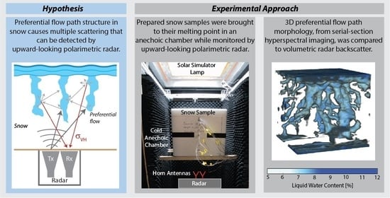
:The infiltration of liquid water in a seasonal snowpack is a complex process that consists of two primary mechanisms: a semi-uniform melting front, or matrix flow, and heterogeneous preferential flow paths. Distinguishing between these two mechanisms is important for monitoring snow melt progression, which is relevant for hydrology and avalanche forecasting. It has been demonstrated that a single co-polarized upward-looking radar can be used to track matrix flow, whereas preferential flow paths have yet to be detected. Here, from within a controlled laboratory environment, a continuous polarimetric upward-looking C-band radar was used to monitor melting snow samples to determine if cross-polarized radar returns are sensitive to the presence and development of preferential flow paths. The experimental dataset consisted of six samples, for which the melting process was interrupted at increasing stages of preferential flow path development. Using a new serial-section hyperspectral imaging method, polarimetric radar returns were compared against the three-dimensional liquid water content distribution and preferential flow path morphology. It was observed that the cross-polarized signal increased by 13.1 dB across these experiments. This comparison showed that the metrics used to characterize the flow path morphology are related to the increase in cross-polarized radar returns spanning the six samples, indicating that the upward-looking polarimetric radar has potential to identify preferential flow paths.
1. Introduction
The initiation of snow melt and the subsequent infiltration of liquid water into a seasonal snowpack are important processes for snow hydrology and avalanche forecasting. The movement of liquid water in a snowpack is generally described as either homogenous matrix flow or heterogenous preferential flow. Homogenous matrix flow describes the slow vertical melting front that initiates at the top of the snowpack and moves vertically downward, semi-uniformly, within the horizontal plane [1]. Preferential flow paths, typically preceding homogenous matrix flow [2], are pathways of concentrated water that can transport large amounts of water vertically through the snowpack [3,4]. When preferential flow paths reach an impermeable layer in the snowpack, such as an ice crust or capillary barrier, water begins to pool and flow laterally [5], which can increase the wet snow avalanche hazard by weakening the snow and lubricating the layer [6]. Observations of preferential flow paths have been predominately made using dye tracers (e.g., [7]), although these types of experiments rely on destructive sampling to visualize a single time step. Although preferential flow paths play a large role in water transport within a snowpack [8], they are challenging to detect and measure.
Non-destructive measurements of snow properties, including wet snow, have been demonstrated using radar, which at longer wavelengths can penetrate through the snow’s volume [9]. For the ground-based radar remote sensing of wet snow, radars have been used in various viewing configurations, including downward-, side-, and upward-looking configurations. Downward-looking radars are limited in wet snow conditions, when the snow surface becomes saturated with water, due to the attenuation and reduced penetration of microwaves [10]. Side-looking radars have been demonstrated to identify preferential flow paths in a natural snowpack by excavating a snowpit and orienting the antennas perpendicular to the snowpit wall [11]; however, this is not a practical method for continuous snow monitoring. A promising configuration for continuous wet snow monitoring has been shown to be the upward-looking radar [12], buried underneath the snowpack, because the attenuation of microwaves does not happen until the melting front reaches the base of the snowpack, and so observations can occur non-destructively over a longer period of time relative to the downward-looking radar at similar wavelengths.
The application of radars in an upward-looking configuration was first demonstrated by Gubler and Hiller [13], which led to additional studies exploring the capability for continuous snowpack monitoring in dry and wet snow conditions. In dry snow, previous retrievals from ground-penetrating radar (GPR) and L-band (1–2 GHz) frequency-modulated continuous wave (FMCW) radar have included the snow height, internal stratigraphy layers, settlement, and density [14,15,16,17,18]. In wet snow conditions, previous retrievals from GPR have included the volumetric liquid water content (LWC) and homogenous matrix flow tracking, as they approached the radar [12].
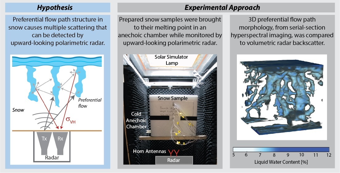
In this previous work, data were primarily collected using a single co-polarized configuration; the radar transmitted and received electromagnetic (EM) waves in the same orientation, either vertical–vertical (VV) or horizontal–horizontal (HH). In this configuration, the co-polarized backscatter (σVV or σHH) is dominated by single scattering returns, which are useful for identifying planar features perpendicular to the antennas that have variations in relative permittivity (), such as the air–snow interface, stratigraphy layers, pooling water on an impermeable layer, and homogenous matrix flow, examples of which are shown in Figure 1a,b. The detection of preferential flow paths has not been demonstrated in the upward-looking configuration, which is likely because the structure and spatial heterogeneity of preferential flow paths do not return a strong and consistent co-polarized signal that can be differentiated from other horizontal layers in the snowpack.
Although not yet having been demonstrated in an upward-looking configuration in wet snow, polarimetric radar data are generally better suited to extract the geometrical structure, shape, and orientation of the target [19], and may have the potential for identifying the presence of preferential flow paths. In addition to co-polarized data, full polarimetric radars include cross-polarized transmit–receive data (i.e., vertical–horizontal (VH) and horizontal–vertical (HV). Cross-polarized backscatter (σVH or σHV) is a result of the incident EM wave being depolarized as a result of multiple scattering events that can occur at the surface due to roughness, or within the volume due to inhomogeneities in the bulk material that contain variations in [20]. Dry snow, consisting of ice and air, has a low , whereas liquid water has a much greater (~88) [21,22]. When preferential flow paths are present, the volume of the snowpack contains large heterogenous variations in , such that multiple scattering events and the subsequent depolarization of an EM wave is probable. The idealized schematic in Figure 1c illustrates the concept behind this hypothesis.
The goal of this study was to test the hypothesis that preferential flow paths within a snow volume can depolarize an incident EM wave, causing an enhanced cross-polarized signal using an upward-looking polarimetric radar. This was tested within a controlled laboratory environment by taking continuous polarimetric radar measurements of prepared snow samples while they were melted from above using a simulated solar lamp. To quantitatively characterize the LWC and morphology of the preferential flow paths, for comparison to the collected radar data, at the end of each experiment, the snow samples were serial-sectioned and LWC maps from hyperspectral imaging were used to create a reconstructed 3D model of the LWC [23].
2. Methods
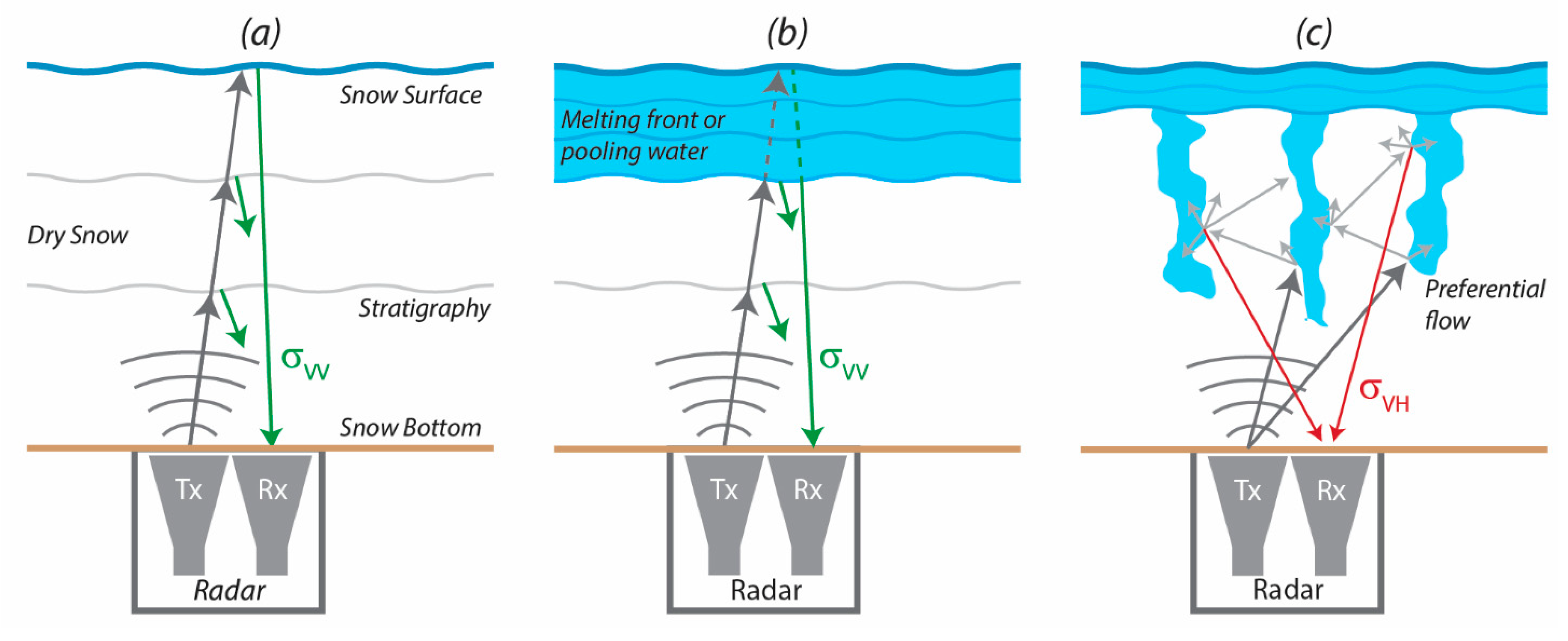
From within a controlled laboratory environment, where prescribed snow structures could be manufactured and characterized, upward-looking polarimetric radar was used to investigate the feasibility of detecting preferential flow paths. Snow samples were prepared and placed underneath a simulated solar lamp to induce melting, while being continuously measured by a C-band (7.29 GHz) radar. The experimental set presented here consisted of six snow samples, each one terminated at progressively increased stages of preferential flow path development. Following termination, the snow samples were near-coincidently serial-sectioned and imaged with a hyperspectral imager before a per-pixel LWC was retrieved across each image using the methodology described in [23]. The stack of serial-section images was reconstructed into a 3D model representing the distribution of LWC within the sample, such that preferential flow paths could be characterized and compared to the radar data. Preferential flow morphology parameters, computed by binarizing the 3D model at different LWC thresholds, were compared against the co- and cross-polarized radar returns integrated over the snow sample volume at the end of the melting experiment (( and ). Additional experimental details are given in Section 2.1, Section 2.2, Section 2.3 and Section 2.4, while an experimental workflow is presented in Figure 2.
2.1. Snow Sample Preparation
Laboratory snow samples were prepared inside of a polystyrene foam container, a material commonly referred to as Styrofoam, because it is nearly invisible to the radar due to its low relative permittivity ( = 1.1). The 42 × 42 × 38 cm (L × W × H) sample container was filled with clean rounded snow grains that were produced in a laboratory snowmaker, similar to the machine described in [24]. The produced snow was stored in a cold room at −10 °C for multiple weeks, which allowed the dendritic crystals to metamorphose into rounded grains of varying sizes. Snow grains were sieved using a 2 mm sieve to create a single homogenous layer within the sample container. The bulk density of the samples, measured by weighing the entire sample, ranged from 370 to 497 kg m−3. The top surface of each sample was scraped with a straight edge to level the snow surface with the top of the sample container. To mitigate edge effects from water flowing down the sides of the sample container along the side walls, the top of the snow sample was shaded along the edge using a piece of polystyrene foam extending 2.5 cm from the sample container side wall. The details for each snow sample are outlined in Table 1.
2.2. Radar Experimental Setup and Raw Data Processing
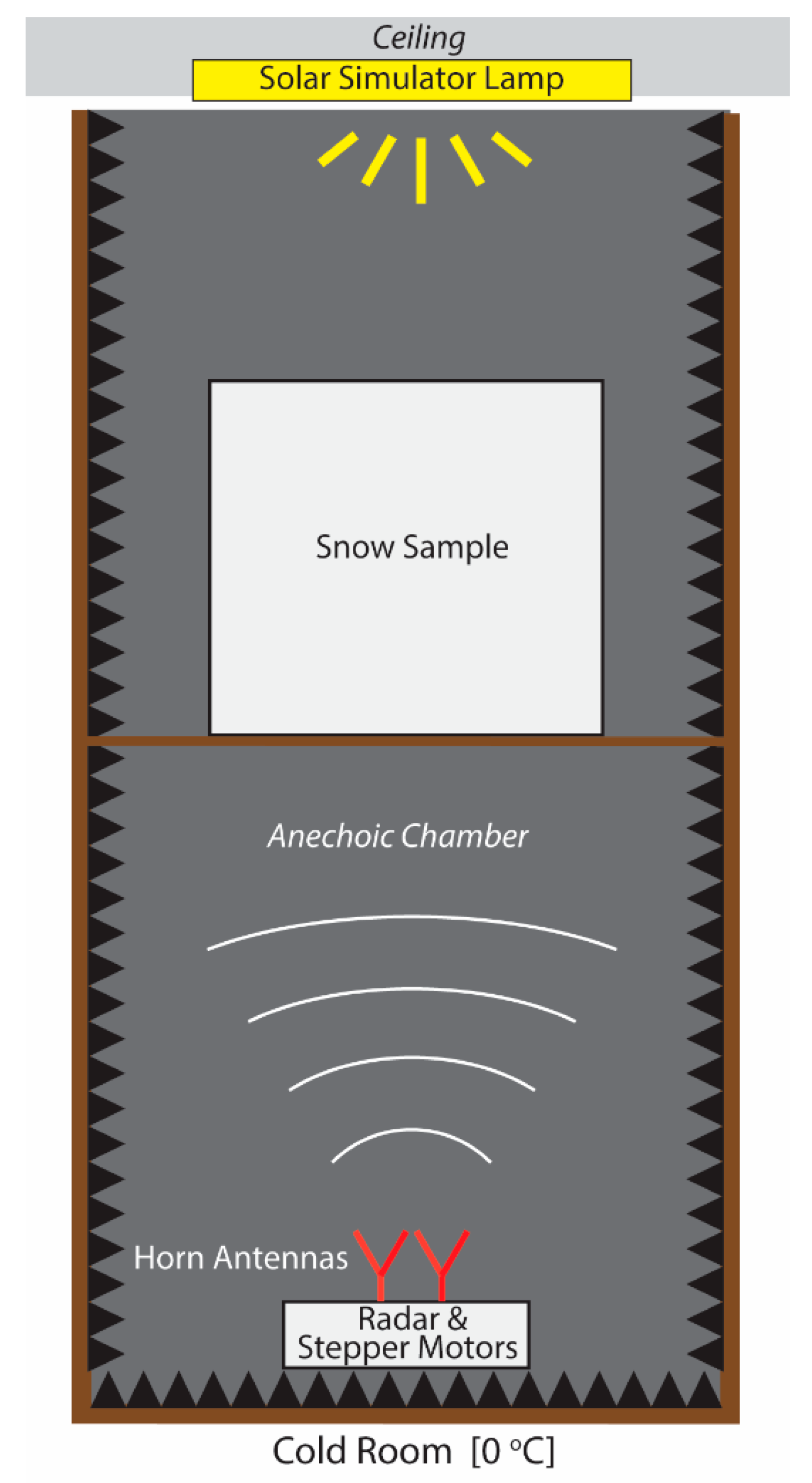
To reduce radar reflections from the walls inside the cold room, each snow sample was placed inside of a custom-built anechoic chamber, represented in Figure 3. The frame of the anechoic chamber was built with plywood, to dimensions of 95 × 95 × 200 cm (L × W × H), and the interior walls were lined with 7.6 cm thick convoluted foam absorbers (Mast Technologies MF32-0002-01) designed to attenuate microwaves at frequencies ranging from 1 GHz to 18 GHz. The top of the anechoic chamber was left open, and the chamber was located underneath a programmable metal halide lamp that simulates the solar spectrum. The shortwave radiation flux of the lamp was set to 900 W m−2, which is a flux commonly observed in spring when seasonal snowpacks undergo melting [25]. Snow samples were placed in the center of the chamber, 41 cm below the solar lamp, on an integrated shelf built into the chamber. The radar was located at the base of the chamber with the antennas pointing upward 75 cm from the bottom of the snow sample.
This study used a SensorLogic Onza ultra-wideband (UWB) radar development kit, which integrates the Novelda XeThru X4 radar technology onto a BeagleBone Black compatible cape. The radar was configured to operate at a center frequency of 7.29 GHz (C-band) with a bandwidth of 1.5 GHz, such that the operating frequency range covered 6.54–8.04 GHz. The radar unit was configured in a quasi-monostatic configuration consisting of two linearly polarized 15 dBi gain horn antennas (WR-137) designed to operate between 5.85 and 8.20 GHz. The far field radiation pattern of the antennas, defined by the Fraunhofer distance [26], was 43 cm, and the bottom of the snow sample was also in this region. To collect four polarimetric measurements (VV, HH, VH, HV), the two antennas were mounted 11 cm apart on a custom-built stepper motor assembly that automatically rotated the antennas through precise 90° rotations between each radar acquisition, such that the antennas were either parallel or orthogonal to each other. During the melt experiment, continuous radar measurements were obtained. At each antenna configuration, twenty radar traces were collected and averaged for that time step. Each polarization measurement and subsequent antenna rotation took 15 s, with all four polarizations collected in approximately 60 s.
Each melt experiment started with the snow sample isothermal at −1 °C, such that the snow sample was dry (i.e., no liquid water) and the cold content was nearly depleted. First, the radar was turned on to collect three full polarimetric measurements of the snow sample in the dry state. Next, the solar lamp was turned on to begin the melting process. By visual inspection of the real-time radar data, melt experiments were terminated at various stages of melt progression to obtain a set of samples that captured a range of preferential flow path sizes and patterns that could be compared to the radar signal.
Post-processing steps were identical for all radar traces. The received signal was normalized to an absolute voltage value between 0 and 1.2 V. To reduce noise, two processing steps were applied; (1) a background signal taken without a snow sample in the anechoic chamber was removed from each radar trace in the frequency domain, and (2) a bandpass filter spanning the frequency range of the radar (5.65–8.04 GHz) was used to remove high and low-frequency noise [27]. Following the processing steps used in [14], a linear time-varying gain was applied to signals to enhance the upper regions of the snow sample that were impacted by radar range loss. For visualization in a radargram format, the processed signal was enveloped using a Hilbert transform [28].
Using a simplified form of the snow radar backscatter model [29], the total radar backscatter received at the antenna for each transmit–receive polarization p and q was decomposed into three components:
where is the backscatter at the air–snow interface at the top of the snow sample, is the backscatter from the snow volume, and is the backscatter at the polystyrene foam–snow interface at the bottom of the snow sample. Of particular interest in this study was the volume component (), because that is where the preferential flow paths develop. To calculate and , the magnitude of the radar signal was integrated over range bins (i.e., fast time) that represented the snow volume. Using the strong co-polarized returns from the top and bottom of the snow samples, the limits of the range bins representing the volume were selected by picking the signal minima following the top and bottom snow surface reflections. Due to the six snow samples having variations in bulk density (370–497 kg m−3), this methodology resulted in the number of range bins to vary by approximately 2 cm (43–47 total range bins) between samples. To not introduce a bias due to the total number of range bins that were integrated, the smallest number of range bins (43 range bins) was used for all samples. In the denser samples, where the number of range bins was larger, the volume range was centered in the middle of the volume, which resulted in at most 2 bins (~1 cm) being excluded on each end.
The characterization of preferential flow paths using the serial-section hyperspectral imaging method, discussed further is Section 2.3, only captured the approximate state of the preferential flow paths within the snow volume at the final time step of the continuous radar measurements. The morphology parameters were compared to and , calculated at the final timestep of the continuous radar measurements, and denoted as and . Of particular interest was the comparison to , given that it would indicate multiple scattering from the presence of preferential flow paths. Since there were no continuous quantifiable preferential flow morphology parameters that could be collected during the melt experiment, the radar data prior to the final time step could only be qualitatively assessed against the final state of the preferential flow paths.
2.3. Serial-Section Hyperspectral Imaging and Data Cube Processing
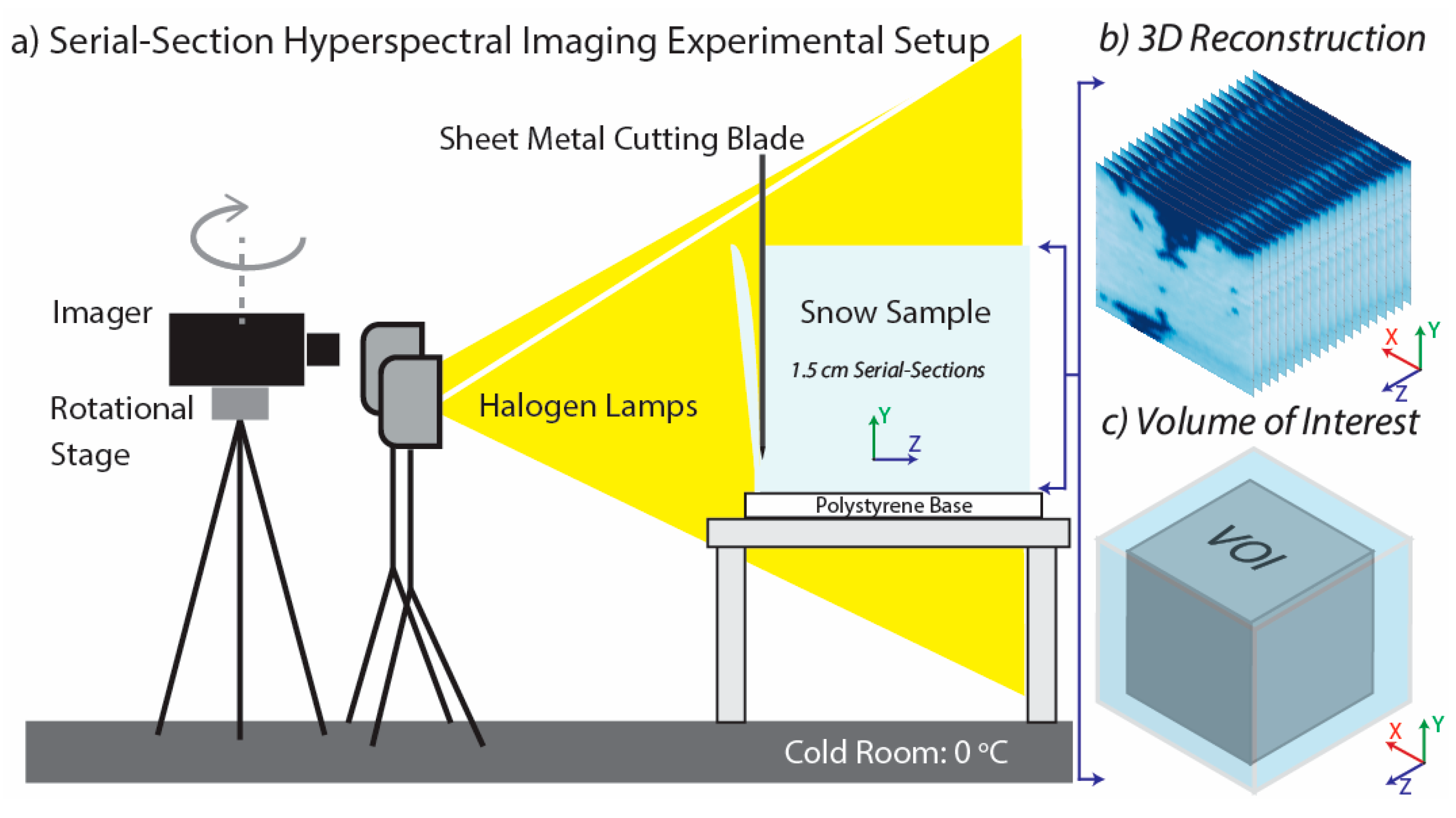
For 3D visualization and quantification of preferential flow paths within the snow volume, each sample was serial-section imaged using a compact hyperspectral imager (Figure 4a). Inside the cold room, set at 0 °C, the sidewalls of the sample container were removed to expose the snow sample. The sample was cut along the vertical profile in ~1.5 cm intervals using a sharpened piece of aluminum sheet metal (60 × 60 cm) that extended beyond the edges of the sample. Following each cut, the snow sample was moved ~1.5 cm towards the imager to maintain a consistent distance between the snow surface and the imager, which maintained a consistent pixel resolution for each image. Each sample was serial-sectioned into 28–33 sections. Following the experimental setup detailed in [30] and briefly described here, each exposed face was illuminated using two diffuse halogen lamps. A Resonon Pika NIR-320 hyperspectral imager was mounted onto a tripod-mounted rotational stage to collect the NIR spectral radiance in each pixel from 900 to 1700 nm. A Spectrolon® 99% reflectance calibration target was placed in the scene of each image to convert each pixel from radiance to bidirectional reflectance.
Following the methodology detailed in [23], the spectral shift in NIR reflectance between ice and liquid water was leveraged to retrieve volumetric LWC on a pixel-by-pixel basis (1.3 mm pixel resolution). Each image contained 315 × 285 (W × H) pixels with LWC values ranging from 0 to 25% LWC and the stack of images was reconstructed into a 3D model with each voxel representing the LWC in the snow sample (Figure 4b). The high pixel resolution in the imaging/cutting plane (x–y, Figure 4) was maintained and each image in the stack was stretched in the cutting direction (z, Figure 4) to represent ~1.5 cm, resulting in a 3D model containing 315 × 315 × 285 voxels (L × W × H) with 2.4 mm3 resolution. A 3D box filter [31], with a filter size of 9, was used to make the edges between voxels continuously smooth.
Within the 3D model, a smaller volume of interest (VOI, gray volume in Figure 4c) was extracted that contained only the preferential flow paths inside the volume of the snow sample and was used to quantify morphology parameters for comparison to the radar signal, discussed further in Section 2.4. In order to only evaluate the contribution from the preferential flow paths, the VOI excluded the top 3.5 cm that included the matrix flow, the bottom 2 cm that included pooling water at the bottom of the sample container, and 3.5 cm from the snow sample edge to remove edge effects. The same VOI dimensions were used for all samples, which contained 262 × 262 × 245 voxels.
2.4. Preferential Flow Morphology
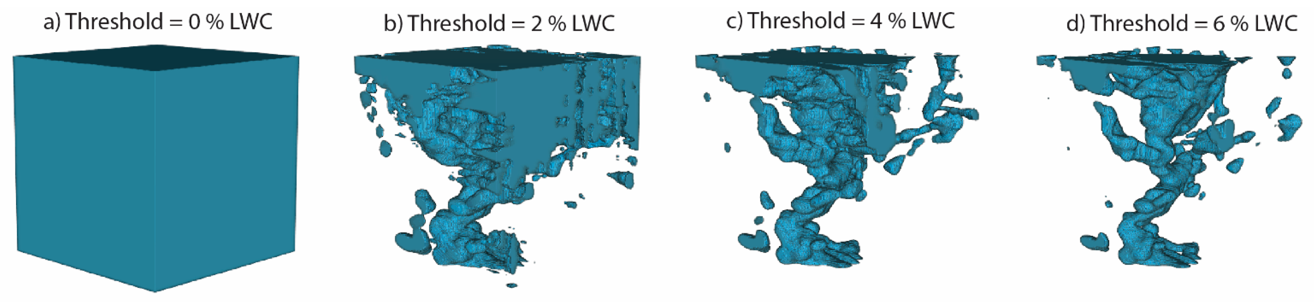
The preferential flow path morphology within the VOI was used as a comparison to and . To calculate morphology parameters, the 3D LWC model had to be in a binarized form, such that the preferential flow paths were represented as objects. Using a LWC threshold, the 3D structure was binarized into an object at 1% steps ranging from 0% to 7% LWC. At a 0% LWC threshold, all voxels were included as part of the object, which resulted in a cube the size of the VOI (Figure 5a). As the threshold was step-wise increased, all voxels containing LWC values of less than the threshold were removed from the object, and the preferential flow paths with higher LWC values were revealed. For example, in Figure 5b–d, the threshold was increased from 2 to 6% LWC, and with each threshold increase, the preferential flow paths became more defined.
Morphology parameters were calculated using the Bruker CT Analyzer (CTAN) software package, an X-ray-computed microtomography (micro-CT) 3D image analysis software. The 2D binarized image stacks were loaded into the program and 3D morphology parameters were computed for each sample at each threshold. The morphology analysis focused on three parameters that quantitatively described the structure of the preferential flow paths: (1) object volume, (2) object surface area, and (3) object separation distance. Object separation is a measure of the mean thickness of open space or cavities that separate the object structures, which is determined by fitting spheres within the open space [32].
3. Results
3.1. Upward-Looking Radar Observations
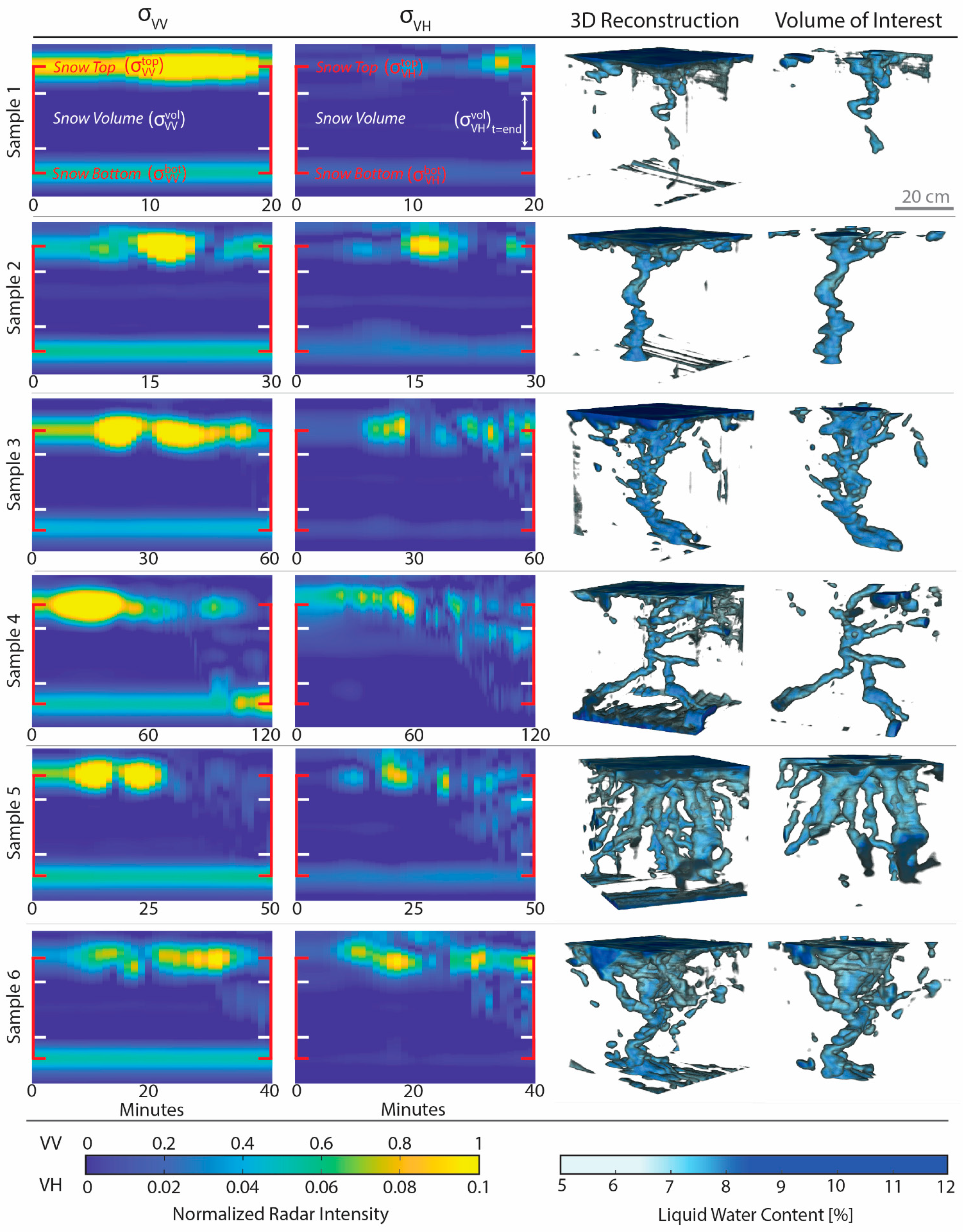
The continuous radar measurements for σVV and σVH are presented in radargrams for each snow sample in columns one and two of Figure 6, respectively, and it is important to note that the color scale for σVV is an order of magnitude greater than σVH. The snow samples were ordered (1–6) in an increasing magnitude of , which are shown in Table 2, and did not consistently correspond to the duration of each experiment. The red tick marks indicate the location of the peak backscatter from the top ( and bottom ( of the snow samples, and the region between the white tick marks represents the limits of the range bins that were integrated to compute the backscatter within the sample volume (). Although σHH and σHV were also collected, they were not presented here, because they were nearly identical to σVV and σVH, given that the radar was in an orthogonal orientation relative to the snow sample.
Generally, and as expected, σVV captured single scattering returns from surfaces that were perpendicular to the antennas, which were the top and bottom surfaces of the snow sample and pooling layers of water. At the start of the experiments, when the snow was dry, σVV detected the top and bottom of the snow sample, with negligible returns within the snow volume (Figure 6, column one). In all samples, melting initiated at the top snow surface at approximately 10 min, which caused to increase due to the introduction of water, increasing . As the melting progressed and water began to percolate through the snow volume, generally began to decrease. In Samples 1–3, remained low relative to and across the duration of each experiment, suggesting minimal single scattering returns from preferential flow paths. Samples 4–6 exhibited higher returns at late stages of the experiment, suggesting an increase in single scattering returns from the increasing preferential flow path cross-sectional area. This was discussed in terms of preferential flow path morphology in Section 4.2. For comparison, and are summarized in Table 2.
In comparison to σVV, σVH had relatively low-magnitude returns at the top and bottom surfaces in dry conditions, which were not present in all samples (e.g., Samples 4–5 at 0 min). As the top of the sample began to melt, as seen in , also increased, although the returns were time-delayed compared to , which was likely due to the returned EM waves being multi-scattered by irregularities in the wet surface. Interestingly, exhibited in all samples at the snow surface and discussed further in Section 4.1, there were periods where faded, while enhanced. As the melting progressed further, enhanced and appeared to track water movement within the snow sample, which supported the hypothesis that the heterogenous nature of preferential flow paths has a depolarizing effect on incident EM waves.
3.2. Liquid Water Content 3D Reconstructions
The 3D LWC reconstructions, shown in Figure 6 (third column), show the main features of water movement through the snow sample. The structures are shown with a 5% LWC threshold; all voxels with LWC < 5% are transparent, and the remaining voxels LWC values are indicated using the color scale. Generally, all samples had a similar structure, including a homogenous matrix flow at the top of the snow surface, preferential flow paths in the snow volume, and varying amounts of pooling water at the bottom of the sample container.
Example VOIs, the portion of the sample used to characterize the structure, are also shown in Figure 6 (fourth column). The VOIs retained the preferential flow path structure, while removing the pooling water at the surface and base of the sample and edge effects. By visual inspection, the preferential flow paths from Samples 1–6 were progressively more complex, which generally coincided with the sample ordering based on the increasing . This result suggests that was sensitive to the development of the preferential flow paths prior to the final time step of the melting experiments, because appeared to correspond with the timing of water percolation in the snow volume.
3.3. Preferential Flow Path Morphology
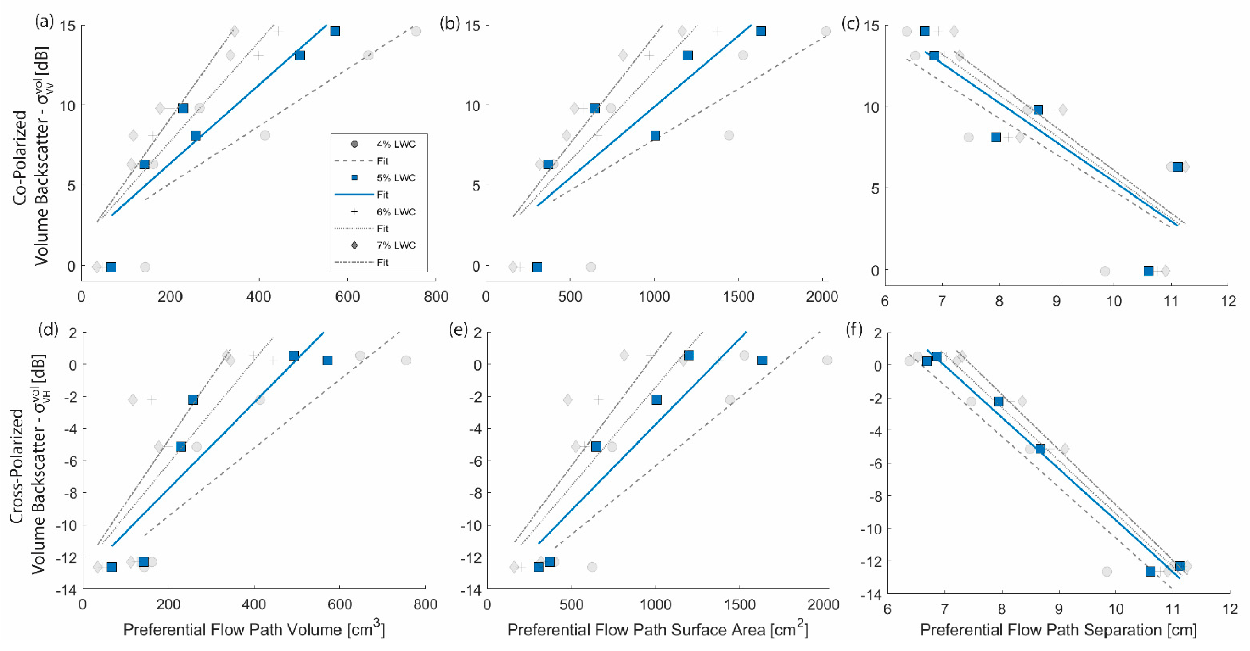
In combination, the 3D LWC models and radar data indicated that the development of preferential flow paths created opportunities for single and multiple scattering, increasing and . The preferential flow path morphology, characterized by volume, surface area, and separation distance, exhibited linear relationships with and at the LWC thresholds between 4 and 7%. At the lower thresholds (1–3%), the flow path structures were not fully resolved (see Figure 5a,b) and R-squared values were low (Table 3). Overall, the morphology parameters for had the best fit (R-squared) at 5% LWC threshold and 7% LWC threshold for . The 5% LWC threshold was represented in blue in Figure 7 and used to visualize the 3D structure in Figure 5.
As shown in Figure 7, the preferential flow volume and surface area had positive trends with and . At each threshold, the volume and surface area had similar trendlines, but shifted to smaller values as the threshold increased and more of the object was removed. These relationships made intuitive sense, because as more preferential flow paths were developed, the likelihood of single and multiple scattering increased. However, the increase in alone could not be used to infer a preferential flow path development because the single scattering returns indicated an increase in the radar cross-section, which could be caused by the matrix or preferential flow. Our data indicated that in combination with , the backscatter could be categorized as preferential flow paths based on multiple scattering returns from the complex structure.
The preferential flow path separation distance had a strong negative relationship with , which indicated that structures that were closer together had a higher likelihood of causing multiple scattering, while structures further apart were less likely to cause multiple scattering and subsequent depolarization. This relationship was also present for , but was notably weaker (Table 3). The trendlines for the separation distance at different LWC thresholds were similar, but shifted to larger separation distances at higher thresholds due to more of the object having been removed.
4. Discussion
4.1. Radar Response from the Top of the Snow Sample
Due to the melt initiation, there was a strong exhibited in all snow samples, which was followed by a period during which weakened, while coincidentally strengthened (Figure 6). In Samples 2–6, this period was then followed by weakening, while strengthened again. To investigate the snow structure and LWC distribution that caused this radar response, the Sample 1 experiment was terminated within this period. Although it was challenging to determine the exact cause of this response by visual inspection of the 3D LWC model in Sample 1, we hypothesized that this time coincided with the period where the top snow layer became sufficiently saturated to overcome capillary forces, and due to gravity began to drain below the snow’s surface [33]. This process had two effects on the radar response: (1) the LWC at the snow surface was reduced, lowering , and, therefore, (2) the underside of the snow surface developed heterogenous distributions of water (Figure 6, Sample 1), similar to surface roughness, and the high variation in increased multiple scattering, strengthening .
4.2. Radar Response from the Snow Volume
Single scattering radar returns typically produce large magnitude peaks and are easy to classify, whereas cross-polarized returns due to multiple scattering within a volume can appear noisy and are challenging to interpret. Here, we discussed volume backscatter in terms of the relative magnitude used in Figure 6, since the co-polarized and cross-polarized return intensity were presented on different scales of normalized intensity. Viewing the co-polarized return intensity on the same scale as the cross-polarized would result in the radargram being over-saturated, due to the large magnitude returns from and . The cross-polarized returns from the experiments presented here generally did not have large magnitude peaks, but rather displayed multiple low-magnitude peaks over the volume region. However, the returns appeared to track the progression of melt toward the bottom of the sample. Although it was not possible to quantify the state of the preferential flow path development within the snow volume during the continuous radar measurements, some qualitative explanations of the volume returns could be determined based on the final 3D LWC model.
In Samples 1 and 2, and were both relatively low, likely due to the preferential flow paths being undeveloped (Sample 1) or in a simple columnar form with no complexities (Sample 2). In Sample 3, was negligible, while tracked the development of the preferential flow paths, which was more complex than Sample 2. This sample was a good example of the cross-polarized radar response being sensitive to complex preferential flow paths, while it was not obvious in the co-polarized returns. In Sample 4, there were unique horizontal preferential flow path features that were not present in other samples, which seemed to be detected by and . Sample 5 had the greatest number of individual preferential flow paths that were spatially distributed in the sample volume, which caused a large , while was small. This result suggested that the spatially distributed preferential flow paths depolarized the incoming radar signal, while the cumulative radar cross-section was not large enough for obvious single scattering returns (). In Sample 6, the returns from and visually looked similar, which could be due to the relatively wide funnel shape that was created by the preferential flow paths that could cause single and multiple scattering returns.
Although had a general increasing trend with the preferential flow path complexity, similar to (Table 2), it would not be possible to solely use this signal to classify the returns as anything other than a horizontal layer of pooling water. Layers containing pooling water in the horizontal plane resulted in strong co-polar returns and negligible cross-polar returns. Conversely, the preferential flow paths resulted in weak co-polar returns and strengthened the cross-polar returns (Figure 6), indicating that the combination of radar returns could be used to classify this process.
4.3. Uncertainties
4.3.1. Polarimetric Radar Measurements
In single antenna (mono-static) polarimetric radars, the system switches between channels to send and receive EM waves in different polarizations, which can introduce cross-talk and gain imbalances between polarization channels. To interpret the data held in polarimetric radar returns, these need to be corrected by using calibration targets because many analysis methods depend on magnitudes and ratios of each polarization [34]. Here, a quasi-monostatic configuration was used that consisted of two antennas wired to separate transmit and receive ports, which minimized cross-talk. Additionally, instead of switching between channels, this radar setup rotated one antenna 90° relative to the other, maintaining an identical gain between polarization measurements. Although a calibration target was not used here, the polarimetric measurements were relative to each other and still represented the polarimetric response observed during the snow melt experiments.
4.3.2. Serial-Sectioning and 3D Reconstruction
Generating the 3D LWC models from serial-section images introduced uncertainties in the spatial distribution of water. To generate the 3D model, each LWC map in the imaging plane (x–y axes in Figure 4) was stretched in the cutting direction (z-axis in Figure 4) to represent ~1.5 cm of depth in the model. This resulted in the resolution of LWC in the x–y axes being 10× higher than in the z-axis, though it allowed for the high-resolution detail of the mapped LWC to be maintained. This approach introduced uncertainty in LWC along the z-axis because the reconstruction assumed that the images are representative of LWC across the 1.5 cm serial-sections. However, this is a reasonable approach, because the penetration of NIR light into snow is approximately 1–2 cm [35].
Under laboratory conditions, the LWC retrieval from NIR hyperspectral imaging had an uncertainty of ~1% LWC by volume [23]. This level of uncertainty could impact the binarized morphology of the preferential flow paths delineated during the LWC thresholding. The incremental threshold changes of 1% LWC, though, resulted in relatively minor changes to the morphology parameters. The exception to this was at the transition from 0% to 1% (dry to the wet snow transition), where there was a large change in binarized morphology (Figure 5). Still, of most relevance to this analysis, the trendlines exhibited in the morphology parameters were maintained across thresholds ranging from 4 to 7%, which indicated that the radar response was dominated by areas of increased LWC.
4.3.3. Morphology Analysis
The LWC thresholding method used in the morphology analysis simplified the actual distribution of LWC in the sample; however, this process was necessary to quantify the preferential flow path morphology. By visual inspection, the preferential flow path morphology was well represented at thresholds between 4 and 7% LWC, which was where trends were found between and the morphology parameters. Although radars operating at C-band are sensitive to lower LWC values (1–3%), there were no morphology trends found, suggesting that larger quantities of water dominated the radar response compared to lower values.
4.4. Outlook for Application in the Field
Radar frequency plays a large role in the measured response from a snowpack. Previous field studies used an upward-looking GPR system, which operates at a lower frequency (0.9 GHz) compared to the C-band (7.29 GHz) radar used here. Due to the long wavelength (~33 cm), GPR systems can penetrate deeper into wet snow, but are less likely to scatter at features smaller than the wavelength. Although not investigated here, it is unlikely that preferential flow paths would cause a similar cross-polarized radar response for GPR. In comparison, the C-band radar has a shallower penetration into wet snow, but the ~5 cm wavelength is more likely to scatter at smaller features, which is better suited for detecting preferential flow paths in the field.
Another important consideration for field application is to recognize the limitations of the laboratory experiments because they represent simplified conditions relative to those found in natural environments. For example, solar diurnal cycles cause a snowpack to go through melt–freeze cycles, where the snowpack is wet during the day and refreezes overnight. This process causes a gradual transition from preferential to matrix flow regimes as spring melting progresses [2], which was not tested in the laboratory. In these transitional conditions, it could be harder to classify which flow regime is present or dominating. Additionally, the complexity of a seasonal snowpack’s stratigraphy is not represented by the homogenous single layer snow volume prepared in a laboratory. Seasonal snowpacks contain stratigraphic layers, ice crusts, and capillary barriers that can impede the vertical movement of water in a preferential flow path, causing pooling or the horizontal diversion of water away from the upward-looking radar. The presence of pooling water causes strong single scattering returns, which would predominately enhance σVV. Detecting a preferential flow would also rely on it developing directly above the radar antenna, which is a function of both the complex radiation exchange and stratigraphic layering.
Still, this work indicated that the upward-looking polarimetric radar could be helpful for identifying structural features within the snow volume that indicate the state of snow melt progression, given that preferential flow typically precedes matrix flow within the snow volume, which would not be possible with a single co-polarized radar. Knowledge of snowmelt progression and structure would be useful for specific applications, for example, differentiating the preferential from matrix flow in avalanche starting zones to inform avalanche forecasting and mitigation efforts. Additionally, if installed at a snow study plot, it could be used to monitor mid-winter melt events and the transition from preferential to matrix flow in spring to inform snowmelt timing.
5. Conclusions
Under controlled laboratory conditions, snow samples were melted by a simulated solar lamp while being continuously measured with an upward-looking polarimetric radar. Six snow samples were analyzed that captured the progression of the preferential flow path development with increasing complexity. Using a new hyperspectral serial-section imaging technique, preferential flow paths were characterized in 3D, such that the morphology could be related to the cross-polarized radar signal. We found that:
- Within a snow volume, the co- and cross-polarized radar responses from an upward-looking UWB (C-band) radar were sensitive to an increasing presence of liquid water, with the cross-polarized signal indicating multiple scattering from water flowing in preferential flow paths.
- A new serial-section hyperspectral imaging method, presented here for the first time, was able to quantify the 3D LWC distribution and preferential flow morphology within a snow sample in high resolution.
- Incremental increases in the development and complexity of the preferential flow paths (Samples 1–6), as defined by morphology parameters, resulted in an overall increase of 14.7 dB in and 13.1 dB in .
- The preferential flow path morphology parameters of object volume and object surface area exhibited linear relationships with and , whereas the object separation distance exhibited a strong linear relationship with only.
This work demonstrated that there is value in having both co-polarized and cross-polarized capabilities in an upward-looking radar installation. A co-polarized radar is only capable of capturing horizontal–perpendicular features in a snowpack; however, structures in other orientations exist, such as preferential flow paths. A cross-polarized radar provides a supplementary dataset that can be used to better classify radar returns.
Author Contributions
Conceptualization, C.D. and K.H.; methodology, C.D.; software, C.D.; validation, C.D.; formal analysis, C.D.; investigation, C.D.; resources, K.H.; data curation, C.D.; writing—original draft preparation, C.D.; writing—review and editing, C.D. and K.H.; visualization, C.D.; supervision, K.H.; project administration, K.H.; funding acquisition, K.H. All authors have read and agreed to the published version of the manuscript.
Funding
This research was funded by the National Aeronautics and Space Administration (NASA), grant number 80NSSC18K0822.
Data Availability Statement
Data available upon request from lead author.
Acknowledgments
The radar and hyperspectral imager used in this study were provided by SensorLogic and McKenzie Skiles, respectively. We would like to thank HP Marshall and Will Tidd for engaging in many conversations about radar. We would also like to thank Ladean McKittrick, McKenzie Skiles, Michael Dvorsak, Evan Schehrer, and Khristian Jones for their assistance in the laboratory. We acknowledge the use of the Subzero Research Laboratory in the Department of Civil Engineering at Montana State University.
Conflicts of Interest
The authors declare no conflict of interest.
References
- Marsh, P.; Woo, M.K. Wetting front advance and freezing of meltwater within a snow cover: 1. Observations in the Canadian Arctic. Water Resour. Res. 1984, 20, 1853–1864. [Google Scholar] [CrossRef]
- Webb, R.; Williams, M.W.; Erickson, T. The spatial and temporal variability of meltwater flow paths: Insights from a grid of over 100 snow lysimeters. Water Resour. Res. 2018, 54, 1146–1160. [Google Scholar] [CrossRef]
- Colbeck, S.C. Water flow through heterogeneous snow. Cold Reg. Sci. Technol. 1979, 1, 37–45. [Google Scholar] [CrossRef]
- Schneebeli, M. Development and stability of preferential flow paths in a layered snowpack. IAHS Publ. Ser. Proc. Rep. Int. Assoc. Hydrol. Sci. 1995, 228, 89–96. [Google Scholar]
- Eiriksson, D.; Whitson, M.; Luce, C.H.; Marshall, H.P.; Bradford, J.; Benner, S.G.; Black, T.; Hetrick, H.; McNamara, J.P. An evaluation of the hydrologic relevance of lateral flow in snow at hillslope and catchment scales. Hydrol. Process. 2013, 27, 640–654. [Google Scholar] [CrossRef]
- Perla, R.I.; Martinelli, M. Forest Service. In Avalanche Handbook; US Department of Agriculture: Washington, DC, USA, 1976. [Google Scholar]
- Williams, M.W.; Erickson, T.A.; Petrzelka, J.L. Visualizing meltwater flow through snow at the centimetre-to-metre scale using a snow guillotine. Hydrol. Process. 2010, 24, 2098–2110. [Google Scholar] [CrossRef]
- Webb, R.W.; Fassnacht, S.R.; Gooseff, M.N. Hydrologic flow path development varies by aspect during spring snowmelt in complex subalpine terrain. Cryosphere 2018, 12, 287–300. [Google Scholar] [CrossRef] [Green Version]
- Marshall, H.-P.; Koh, G. FMCW radars for snow research. Cold Reg. Sci. Technol. 2008, 52, 118–131. [Google Scholar] [CrossRef]
- Marshall, H.P.; Koh, G.; Forster, R.R. Ground-based frequency-modulated continuous wave radar measurements in wet and dry snowpacks, Colorado, USA: An analysis and summary of the 2002–03 NASA CLPX data. Hydrol. Process. 2004, 18, 3609–3622. [Google Scholar] [CrossRef]
- Albert, M.; Koh, G.; Perron, F. Radar investigations of melt pathways in a natural snowpack. Hydrol. Process. 1999, 13, 2991–3000. [Google Scholar] [CrossRef]
- Mitterer, C.; Heilig, A.; Schweizer, J.; Eisen, O. Upward-looking ground-penetrating radar for measuring wet-snow properties. Cold Reg. Sci. Technol. 2011, 69, 129–138. [Google Scholar] [CrossRef]
- Gubler, H.; Hiller, M. The use of microwave FMCW radar in snow and avalanche research. Cold Reg. Sci. Technol. 1984, 9, 109–119. [Google Scholar] [CrossRef]
- Heilig, A.; Schneebeli, M.; Eisen, O. Upward-looking ground-penetrating radar for monitoring snowpack stratigraphy. Cold Reg. Sci. Technol. 2009, 59, 152–162. [Google Scholar] [CrossRef]
- Schmid, L.; Heilig, A.; Mitterer, C.; Schweizer, J.; Maurer, H.; Okorn, R.; Eisen, O. Continuous snowpack monitoring using upward-looking ground-penetrating radar technology. J. Glaciol. 2014, 60, 509–525. [Google Scholar] [CrossRef] [Green Version]
- Heilig, A.; Mitterer, C.; Schmid, L.; Wever, N.; Schweizer, J.; Marshall, H.-P.; Eisen, O. Seasonal and diurnal cycles of liquid water in snow—Measurements and modeling. J. Geophys. Res. Earth Surf. 2015, 120, 2139–2154. [Google Scholar] [CrossRef] [Green Version]
- Heilig, A.; Eisen, O.; Schneebeli, M. Temporal observations of a seasonal snowpack using upward-looking GPR. Hydrol. Process. 2010, 24, 3133–3145. [Google Scholar] [CrossRef]
- Okorn, R.; Georg, B.; Thomas, P.; Achim, H.; Lino, S.; Christoph, M.; Jürg, S.; Olaf, E. Upward-looking L-band FMCW radar for snow cover monitoring. Cold Reg. Sci. Technol. 2014, 103, 31–40. [Google Scholar] [CrossRef] [Green Version]
- Lee, J.-S.; Pottier, E. Polarimetric Radar Imaging: From Basics to Applications; CRC Press: Boca Raton, FL, USA, 2017. [Google Scholar]
- Cloude, S. Polarisation: Applications in Remote Sensing; OUP Oxford: Oxford, UK, 2009. [Google Scholar]
- Matzler, C. Microwave permittivity of dry snow. IEEE Trans. Geosci. Remote Sens. 1996, 34, 573–581. [Google Scholar] [CrossRef]
- Archer, D.G.; Wang, P. The dielectric constant of water and Debye-Hückel limiting law slopes. J. Phys. Chem. Ref. Data 1990, 19, 371–411. [Google Scholar] [CrossRef] [Green Version]
- Donahue, C.; Skiles, S.M.; Hammonds, K. Mapping liquid water content in snow at the millimeter scale: An intercomparison of mixed-phase optical property models using hyperspectral imaging and in situ measurements. Cryosphere 2022, 16, 43–59. [Google Scholar] [CrossRef]
- Schleef, S.; Matthias, J.; Henning, L.; Martin, S. An improved machine to produce nature-identical snow in the laboratory. J. Glaciol. 2014, 60, 94–102. [Google Scholar] [CrossRef] [Green Version]
- Skiles, S.M.; Painter, T. Daily evolution in dust and black carbon content, snow grain size, and snow albedo during snowmelt, Rocky Mountains, Colorado. J. Glaciol. 2017, 63, 118–132. [Google Scholar] [CrossRef] [Green Version]
- Walter, C.H. Traveling Wave Antennas; Dover Publications: New York, NY, USA, 1970. [Google Scholar]
- Shenoi, B.A. Introduction to Digital Signal Processing and Filter Design; John Wiley & Sons: Hoboken, NJ, USA, 2005. [Google Scholar]
- Bracewell, R.N. The Fourier Transform and Its Applications; McGraw-Hill: New York, NY, USA, 1986; Volume 31999. [Google Scholar]
- Ulaby, F.T. Rader remote sensing and surface scattering and emission theory. In Microwave Remote Sensing Active and Passive; Artech House Publishers: Norwood, MA, USA, 1982; pp. 848–902. [Google Scholar]
- Donahue, C.; Skiles, S.M.; Hammonds, K. In situ effective snow grain size mapping using a compact hyperspectral imager. J. Glaciol. 2021, 67, 49–57. [Google Scholar] [CrossRef]
- The MathWorks, Inc. MathWorks, Image Processing Toolbox Reference; The MathWorks, Inc.: Natick, MA, USA, 2022; pp. 1397–1399. [Google Scholar]
- Hildebrand, T.; Rüegsegger, P. A new method for the model-independent assessment of thickness in three-dimensional images. J. Microsc. 1997, 185, 67–75. [Google Scholar] [CrossRef]
- Colbeck, S. A theory of water percolation in snow. J. Glaciol. 1972, 11, 369–385. [Google Scholar] [CrossRef] [Green Version]
- Sarabandi, K.; Ulaby, F.T. A convenient technique for polarimetric calibration of single-antenna radar systems. IEEE Trans. Geosci. Remote Sens. 1990, 28, 1022–1033. [Google Scholar] [CrossRef]
- Nolin, A.W.; Dozier, J. A Hyperspectral Method for Remotely Sensing the Grain Size of Snow. Remote Sens. Environ. 2000, 74, 207–216. [Google Scholar] [CrossRef]
Figure 1.
Idealized schematic of an upward-looking radar configuration in (a) dry snow, (b) melting snow with wetting front, or (c) pooling water preferential flow paths. Single scattering returns are co-polarized (σVV, shown in green), while multiple scattering returns are depolarized and detected with the cross-polarized antenna (σVH, shown in red).

Figure 2.
Laboratory experimental workflow.

Figure 3.
Schematic of laboratory snow melt experiments within an anechoic chamber inside of a cold room with continuous upward-looking polarimetric radar measurements.
Figure 3.
Schematic of laboratory snow melt experiments within an anechoic chamber inside of a cold room with continuous upward-looking polarimetric radar measurements.

Figure 4.
(a) Schematic of serial-section hyperspectral imaging experimental setup inside of cold room. (b) Visualization of a stack of serial-section images reconstructed to represent the 3D distribution of liquid water content in the snow sample. (c) Schematic of the entire volume of the reconstructed snow sample (light blue) and the volume of interest (VOI, gray) within the snow sample volume.

Figure 5.
An example (Sample 6) of binarizing the volume of interest (VOI) using a liquid water content (LWC) threshold equal to (a) 0%, (b) 2%, (c) 4%, and (d) 6%.
Figure 5.
An example (Sample 6) of binarizing the volume of interest (VOI) using a liquid water content (LWC) threshold equal to (a) 0%, (b) 2%, (c) 4%, and (d) 6%.

Figure 6.
The first two columns are the continuous co-polarized and cross-polarized radargram for each melt experiment (Samples 1–6). The snow sample top and bottom are indicated with the red tick marks and the snow sample volume is represented as the area between the white tick marks. For visualization, the color scale for σVV is an order of magnitude greater than σVH. The second two columns are the corresponding 3D reconstruction and volume of interest with the liquid water content threshold set to 5%. Shading was applied to the 3D models to help visualize the structure.

Figure 7.
The morphology parameters, from left to right, preferential flow path volume, preferential flow path surface area, and preferential flow path separation distance derived at liquid water content (%LWC) thresholds ranging from 4 to 7% and plotted versus the (a–c) co- and (d–f) cross-polarized volume component from the final timestep in the melt experiment, and .


Table 1.
Snow sample properties.
| Snow Sample | Density (kg m−3) | Time Under Solar Lamp (min) |
|---|---|---|
| 1 | 497 | 20 |
| 2 | 489 | 30 |
| 3 | 370 | 60 |
| 4 | 399 | 120 |
| 5 | 479 | 50 |
| 6 | 378 | 40 |
Table 2.
Integrated co- and cross-polarized backscatter within the snow sample volume at the final time step of the melt experiment.
Table 2.
Integrated co- and cross-polarized backscatter within the snow sample volume at the final time step of the melt experiment.
| Snow Sample | (dB) | (dB) |
|---|---|---|
| 1 | −0.1 | −12.6 |
| 2 | 6.3 | −12.3 |
| 3 | 9.8 | −5.1 |
| 4 | 8.1 | −2.2 |
| 5 | 13.1 | 0.2 |
| 6 | 14.6 | 0.5 |
Table 3.
Coefficient of determination (R-squared) between the morphology parameters at each liquid water content (LWC) threshold and the co- and cross-polarized volume component at the final timestep in the melt experiment, and . Bold values indicated LWC thresholds that are included in Figure 7.
Table 3.
Coefficient of determination (R-squared) between the morphology parameters at each liquid water content (LWC) threshold and the co- and cross-polarized volume component at the final timestep in the melt experiment, and . Bold values indicated LWC thresholds that are included in Figure 7.
| Co-Polarized | Cross-Polarized | |||||
|---|---|---|---|---|---|---|
| LWC Threshold (%) | Volume | Surface Area | Separation | Volume | Surface Area | Separation |
| 1 | 0.04 | 0.01 | 0.07 | 0.31 | 0.27 | 0.46 |
| 2 | 0.20 | 0.06 | 0.16 | 0.51 | 0.35 | 0.61 |
| 3 | 0.51 | 0.27 | 0.30 | 0.76 | 0.60 | 0.74 |
| 4 | 0.75 | 0.57 | 0.62 | 0.84 | 0.82 | 0.95 |
| 5 | 0.85 | 0.75 | 0.73 | 0.81 | 0.86 | 0.98 |
| 6 | 0.87 | 0.83 | 0.74 | 0.74 | 0.79 | 0.99 |
| 7 | 0.88 | 0.85 | 0.75 | 0.70 | 0.73 | 0.99 |
Publisher’s Note: MDPI stays neutral with regard to jurisdictional claims in published maps and institutional affiliations. |
© 2022 by the authors. Licensee MDPI, Basel, Switzerland. This article is an open access article distributed under the terms and conditions of the Creative Commons Attribution (CC BY) license (https://creativecommons.org/licenses/by/4.0/).
Share and Cite
MDPI and ACS Style
Donahue, C.; Hammonds, K. Laboratory Observations of Preferential Flow Paths in Snow Using Upward-Looking Polarimetric Radar and Hyperspectral Imaging. Remote Sens. 2022, 14, 2297. https://doi.org/10.3390/rs14102297
AMA Style
Donahue C, Hammonds K. Laboratory Observations of Preferential Flow Paths in Snow Using Upward-Looking Polarimetric Radar and Hyperspectral Imaging. Remote Sensing. 2022; 14(10):2297. https://doi.org/10.3390/rs14102297
Chicago/Turabian StyleDonahue, Christopher, and Kevin Hammonds. 2022. "Laboratory Observations of Preferential Flow Paths in Snow Using Upward-Looking Polarimetric Radar and Hyperspectral Imaging" Remote Sensing 14, no. 10: 2297. https://doi.org/10.3390/rs14102297
Note that from the first issue of 2016, this journal uses article numbers instead of page numbers. See further details here.