


Abstract
A leading theoretical expectation for the final stages of planet formation is that disk migration should naturally drive orbits into chains of mean motion resonances (MMRs). In order to explain the dearth of MMR chains observed at Gyr ages (<1%), this picture requires such configurations to destabilize and scramble period ratios following disk dispersal. Strikingly, the only two known stars with three or more planets younger than ≲100 Myr, HR 8799 and V1298 Tau, have been suggested to be in such MMR chains, given the orbits' near-integer period ratios. We incorporate recent transit and radial velocity (RV) observations of the V1298 Tau system, and investigate constraints on the system's orbital architecture imposed by requiring dynamical stability on timescales much shorter than the system's age. We show that the recent RV mass measurement of V1298 Tau b places it within a factor of 2 of the instability limit, and that this allows us to set significantly lower limits on the eccentricity (eb ≤0.17 at 99.7% confidence). Additionally, we rule out a resonant chain configuration for V1298 Tau at ≳99% confidence. Thus, if the ∼23 Myr old V1298 Tau system did form as a resonant chain, it must have undergone instability and rearrangement shortly after disk dispersal. We expect that similar stability constrained characterization of future young multiplanet systems will be valuable in informing planet formation models.
Export citation and abstract BibTeX RIS

Original content from this work may be used under the terms of the Creative Commons Attribution 4.0 licence. Any further distribution of this work must maintain attribution to the author(s) and the title of the work, journal citation and DOI.
1. Introduction
The Kepler mission (Borucki et al. 2010) revealed a broad population of planets smaller than Neptune (≲4 R⊕) in compact orbital configurations (Howard et al. 2012; Petigura et al. 2018). Theoretical studies suggest that planetary systems may have originally formed with higher planetary multiplicity and short lifetimes, and undergone instabilities that rearranged them into more widely spaced and progressively longer-lived configurations (Pu & Wu 2015; Volk & Gladman 2015; Bitsch et al. 2019). Izidoro et al. (2017, 2021) (see also Goldberg & Batygin 2022) additionally argue that dissipative migration in a protoplanetary disk should promote initial formation in chains of mean motion resonances (MMRs) between the planetary orbits, and suggest that subsequent dynamical instabilities could scramble orbital periods, explaining the wide period ratio distribution and dearth of chains of MMRs observed at Gyr ages (Fabrycky et al. 2014; Morrison et al. 2020).
Targeted efforts to find young planetary systems could test this hypothesis by checking whether such systems are preferentially found in resonant chains at early ages. Several such searches are underway, e.g., the Zodiacal Exoplanets in Time survey (Rizzuto et al. 2017) and the Cluster Difference Imaging Photometric Survey (Bouma et al. 2019). Although several young exoplanets have been found, e.g., AU Mic b and c (Plavchan et al. 2020), DS Tuc A b and c (Newton et al. 2019), and K2-33 b (David et al. 2016), there are very few young systems with three or more planets to check for resonant chains.
Intriguingly, for the only two known 3+ planet systems younger than 100 Myr, ∼23 Myr old V1298 Tau (David et al. 2019a, 2019b) and ∼40 Myr old HR8799 (Marois et al. 2008), it has been suggested that both may be in a resonant chain based on their observed period ratios (Wang et al. 2018; Feinstein et al. 2021).
Given that only ∼1% of mature systems with three or more planets are found in MMR chains (Morrison et al. 2020), such a resonant configuration for the youngest multiplanet systems would support the theoretical work of Izidoro et al. (2017), Bitsch et al. (2019), and Izidoro et al. (2021).
However, whether or not these systems are in fact in MMR chains depends on not just the period ratios, but also the planetary masses and orbital eccentricities. While radial velocity (RV) measurements are challenging due to strong activity in the young star V1298 Tau, recent RV measurements by Suárez Mascareño et al. (2021) find a mass for planet b of 0.64 ± 0.19 MJup, and 3σ upper limits for the masses of c and d of 0.24 and 0.31 MJup, respectively. The RV data was taken by the high-resolution spectrographs High Accuracy Radial velocity Planet Searcher-North, the Calar Alto high-Resolution search for M dwarfs with Exoearths with Near-infrared and optical Échelle Spectrographs, the STELLA Echelle Spectrograph, and the High-Efficiency and high Resolution Mercator Échelle Spectrograph between 2019 April and 2020 April (Suárez Mascareño et al. 2021).
The large mass measured for planet b in this compact system implies that many possible orbital configurations would immediately go unstable.
We therefore investigate the constraints imposed by dynamical stability on the masses, orbital parameters, and resonant configuration of the V1298 Tau planets. 1 Our work is informed by the recent RV observations from Suárez Mascareño et al. (2021), and period ratio observations from K2 and TESS transits separated by roughly 6.5 yr (David et al. 2019a; Feinstein et al. 2021). Finally, we discuss the implications of our results for the hypothesis that planets generically form in MMR chains that subsequently destabilize (Izidoro et al. 2017; Bitsch et al. 2019; Izidoro et al. 2021; Goldberg & Batygin 2022).
2. Resonant and Near-resonant Configurations for Planets c and d
The orbital periods of planets c, d, and b (listed in increasing distance from the star, which differs from the order of their discovery) are precisely measured across several transits, with fractional errors ∼10−3 days. The outer planet's (planet e) orbital period is significantly less certain (Pe = 50.29 ± 6.62 days; Feinstein et al. 2021), since only two transits spaced by roughly 6.5 yr have been observed. We ignore planet e in this study due to this uncertainty, and argue in Section 3.5 that for reasonable planet parameters, its omission does not significantly affect our results. We present the known relevant parameters of the V1298 Tau planets in Table 1.
Table 1. V1298 Tau Planet Characteristics
| Planet | Period (days) | Mass (MJup) | Eccentricity |
|---|---|---|---|
| c |

| <0.24 | <0.30 |
| d |

| <31 | <0.20 |
| b |

| 0.64 ± 0.19 | 0.134 ± 0.075 |
Note. Planet periods from Feinstein et al. (2021) with masses and eccentricities from Suárez Mascareño et al. (2021) in descending order of their periods; planet b was discovered first by David et al. (2019b). Note that the period ratio of the first planet pair is consistent with the 3:2 resonance, but the ratio of the next planet pair is interior to the 2:1 resonance; Pb /Pd = 1.946. We leave out the outer planet due to its ambiguous period, justifying this in Section 3.5.
Download table as: ASCIITypeset image
We begin by sampling a wide range of masses, eccentricities and orbital orientations for the inner planets c and d in and near the 3:2 MMR consistent with their observed period ratio ≈1.503, and in the next section explore the constraints imposed by orbital stability in the presence of planet b. Doing the analysis in this two-step process means that our full orbital configurations do not necessarily exactly match all the available orbital period measurements, but greatly clarifies which combinations of parameters are dominantly constrained by stability in the high-dimensional parameter space. Given that Spitzer observations (J. Livingston et al. 2022, in preparation) and further RV analysis (S. Blunt et al. 2022, in preparation) of the system will soon provide new constraints, we defer detailed orbit-fitting to those studies, and provide a framework for incorporating stability requirements.
2.1. Sampling Orbits for Planets c and d near the 3:2 MMR
Planets c and d transited nine and five times during the K2 observations, and four and three times when observed by TESS, roughly 6.5 yr (≈200 orbits) later, respectively. This effectively provides two "instantaneous" measurements of their physically meaningful period ratio: 1.503 ± 0.0001 as measured in 2015 with K2 (David et al. 2019a), and 1.503 ± 0.0005 as measured in 2021 with TESS (Feinstein et al. 2021).
The simplest explanation for the consistent period ratio measurements in the two epochs is that the orbital periods are approximately constant in time, though more general oscillating solutions one might expect near MMRs (see Chapter 8 of Murray & Dermott 1999) are also possible. Most of the techniques for speeding up Markov Chain Monte Carlo parameter estimation methods (e.g., Foreman-Mackey et al. 2013) do not work for sampling the wide and disconnected sets of masses and orbital parameters consistent with two observed period ratios. We therefore opt for a simple rejection sampling approach (e.g., Price-Whelan et al. 2017) where we accept a set of masses and orbital parameters based on the likelihood L of the period ratio passing through the observations: 2

where the ti are the times of the (two) observations, σi the observational uncertainties (assumed Gaussian), pobs are the observed period ratios, and pmodel are the period ratios as determined using the WHFast integrator (Rein & Tamayo 2015) in the REBOUND N-body package (Rein & Liu 2012).
In order to sample a wide range of resonant and near-resonant configurations consistent with the observed period ratios, while reducing the number of parameters and aiding in their interpretation, we exploit analytical models of the planetary dynamics in and near MMRs. In particular, we sample four parameters: the planet pair's total planet–star mass ratio μ = (mc + md )/m⋆, the equilibrium combined eccentricity eforced parameterizing the strength of the 3:2 MMR, the combined free eccentricity efree, measuring how far the planet pair is from the equilibrium value, and the resonant angle ϕ, which measures the azimuthal angle at which conjunctions between the two planets occur, and sets the phase of the period ratio oscillations. The fact that two masses and twelve orbital parameters for the two planets can be approximately distilled into four parameters determining the period ratio evolution is not obvious, so we provide more details in the Appendix. We perform these and all other calculations of resonant parameters in this paper using the open-source celmech package. 3
2.2. Resonant and Near-resonant Configurations
We sampled  and
and  uniformly from 0 to 0.2 (i.e., nearly orbit-crossing), and the total planet–star mass ratio μ log-uniformly. These planets may be significantly inflated (David et al. 2019a), so we adopt a low-mass bound of μ at 3 M⊕ based on measurements of the least dense exoplanet known—Kepler-51b (Steffen et al. 2013; Masuda 2014). For the upper bound, we chose 1 MJup to conservatively account for the RV upper bounds (Suárez Mascareño et al. 2021).
We sampled 60 million configurations, accepting 9693. This posterior size is adequate to explore our parameter space, and is shown in Figure 1, where the dashed histograms are the rejection posteriors. The color-coding and solid histograms incorporate stability constraints and are discussed in Section 3.
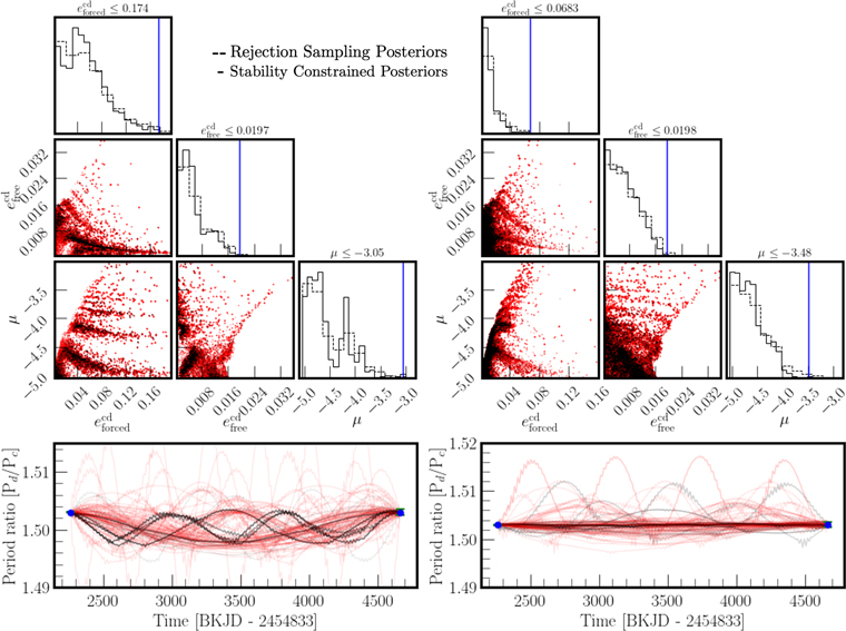
Figure 1. Posterior distribution of orbital configurations for the inner two planets, c and d, based on the two observed period ratios shown in blue in the bottom panels. The left panel shows configurations where the planets are in the 3:2 MMR, and the right panel shows nonresonant configurations. See the end of Section 2.1 for variable definitions. Red configurations go unstable in N-body integrations within ≈225 yr (104 orbits) upon sampling a mass and orbit for planet b from RV observations (Section 3). The dashed histograms trace all of the configurations, while the solid histograms are the stability constrained distributions, i.e., weighted by each configuration's probability of stability as evaluated by the Stability of Orbital Configurations Klassifier (SPOCK; red points have SPOCK probability = 0). The blue solid lines mark the 99.7th percentile upper limit for each parameter. The lower panels show period ratio time series for a 100 random samples, passing through the observations, marked as blue points with their (small) error bars. See the text for discussion.
Download figure:
Standard image High-resolution imageWe divide our configurations into ones that are inside the 3:2 MMR on the left half of Figure 1, and ones that are not (≈78%) on the right (see Appendix A.3 for details). We see that in both the resonant and nonresonant cases, the observed period ratios for planets c and d significantly favor lower masses. In the resonant cases, the forced eccentricities parameterizing the strength of the MMR are higher than in the nonresonance configurations. This reflects the fact that for most of the configurations on the right side of Figure 1, the MMR is weak enough that there is no resonant region at all (Appendix A.3). The oscillations around the equilibrium, parameterized by efree are small in both cases.
We also show the period ratio evolution for a random selection of 100 solutions in the bottom panels with the two observed values in blue. Many of the nonresonant configurations on the right exhibit flat period ratios because the masses and orbital parameters render the MMR weak. For the resonant cases where the MMR is strong, we get finite-amplitude oscillations in the period ratio (the bottom left panel of Figure 1) even if we restrict efree = 0, which by definition should correspond to a configuration at the resonant equilibrium with a constant period ratio. This discrepancy is due to the fact that the analytical MMR model, and its prediction for the location of the resonant equilibrium, is only approximate. Given that the two observations in blue (the bottom panels of Figure 1) are consistent within very narrow error bars (plotted), improved or numerical models would provide a stronger preference for nearly flat period ratio solutions with efree ≈ 0. Since our goal is simply to explore a representative range of resonant and near-resonant configurations for planets c and d in the presence of a massive planet b, we do not pursue this further. A third set of transits for planets c and d would provide a strong and valuable constraint on their resonant configuration, and for whether the period ratio is constant with time.
For the resonant cases (the left side of Figure 1), the configurations most vulnerable to instabilities due to perturbations from other planets are those near the boundaries of the MMR, i.e., near the separatrix (e.g., Rath et al. 2021). The separatrix corresponds to a particular value of efree, or equivalently to the black "cat's-eye" boundary in the plane spanned by ϕ and the period ratio deviation from 1.5 shown in the left panel of Figure 2 (see the Appendix for details). To account for the fact that the size of this resonant region varies with μ and eforced, for each of the resonant configurations, we use celmech to normalize the period ratio deviation by the value at the separatrix so that the MMR boundary for all the resonant configurations plotted in Figure 2 extends from [−1, 1]. We see that while a diffuse distribution of configurations fill the "cat's eye" resonant region, most configurations cluster closer to the equilibrium (equivalently at low efree), with higher mass solutions closer to the equilibrium.
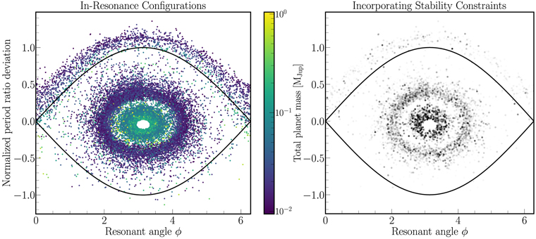
Figure 2. For the resonant configurations on the left side of Figure 1, we plot the 3:2 resonant island for planets c and d, bounded by the "cat's eye" separatrix trajectory (solid black line). The x-axis is the 3:2 resonant angle, and the y-axis is the period ratio's deviation from 3/2. The resonance region varies for each configuration (points) since it depends on the masses and orbital parameters, so the period ratio deviation has been normalized so that the separatrix extends from ≈ [−1, 1] for all points (see the Appendix). The left panel shows the original posterior samples (both black and red points in Figure 1), with the color bar denoting the total planet mass mc + md . The right panel applies stability constraints by setting an opacity to each point given by the SPOCK probability of stability. As expected, stability preferentially removes configurations near the separatrix, but it also imposes additional structure.
Download figure:
Standard image High-resolution image3. Stability Constrained Characterization
With a range of resonant and near-resonant configurations for c and d in hand, we now introduce planet b and determine the constraints imposed by stability. In order to make this step computationally tractable, we use the SPOCK package (Tamayo et al. 2020; Cranmer et al. 2021), a collection of machine learning and analytical models for predicting the stability of compact multiplanet systems.
We randomly draw 105 resonant and near-resonant configurations for planets c and d from the samples generated in Section 2.2 (with replacement), and introduce planet b. We note that, in general, the addition of planet b causes the evolution of the period ratio between c and d to no longer pass exactly through the observed values of 1.503, but we leave detailed orbit-fitting to imminent future observations (J. Livingston et al. 2022, in preparation). Our goal instead is to explore stability constraints for a representative sample of resonant and near-resonant configurations for planets c and d, given the RV mass and orbital eccentricity measured by Suárez Mascareño et al. (2021).
We choose the orbital period of planet b to yield the precisely observed period ratio Pb
/Pd
= 1.946, and draw the masses and orbital eccentricities from the RV posteriors of Suárez Mascareño et al. (2021), assuming Gaussian errors:  ,
,  . Finally, we sample the longitude of pericenter and true longitude of planet b uniformly between 0 and 2π. We then use SPOCK (Tamayo et al. 2020) to calculate the probability of each of the 105 configurations being stable for the next ∼109 orbits. Red configurations in Figure 1 went unstable within 104 orbits (SPOCK probability of zero), and the stability constrained (solid line) histograms weight each sample by its respective SPOCK probability (Tamayo et al. 2021a).
3.1. How Long to Require Stability?
Our approach requires closer examination for this particularly young system, given the possibility that planetary systems may generically be unstable, undergoing dynamical instabilities throughout their lives (e.g., Laskar 1996; Pu & Wu 2015; Volk & Gladman 2015; Izidoro et al. 2017; Bitsch et al. 2019; Izidoro et al. 2021). Nevertheless, in that picture, one might expect a system observed at an arbitrary snapshot in time to always have a time to instability comparable to its present lifetime (Laskar 1996). Thus, even if planetary systems are ultimately unstable, one can still require stability on timescales much shorter than their age, since otherwise instabilities would be happening all the time.
The SPOCK FeatureClassifier (Tamayo et al. 2020) provides a probability of stability over 109 orbits of the innermost planet, corresponding to ≈22 Myr for V1298 Tau. For this young system, that timescale is close to its age, and thus too stringent a timescale on which to require stability.
However, most instabilities occur early, and we do not expect this to significantly bias our results. About 96% of our tested configurations had SPOCK probabilities ≤0.2. We checked the median instability times for these low-probability configurations with SPOCK's deep learning classifier (Cranmer et al. 2021), and found 97% had predicted lifetimes ≤107 orbits (≲0.2 Myr). This preference toward short lifetimes also matches expectations from the analytic investigation of these instabilities by Tamayo et al. (2021b).
3.2. Constraints on Planets c and d
For the nonresonant cases on the right side of Figure 1, stability sets a 99.7th percentile upper limit for the combined mass of planets c and d of μ < 0.35 MJup, slightly more constraining than the upper limits from the RV observations (Suárez Mascareño et al. 2021). Stability of resonant configurations (the left side of Figure 1), on the other hand, allows for values up to 0.95 MJup (99.7th percentile). Moreover, SPOCK shows a preference toward particular values of μ (peaks in the solid histogram for μ, the lower right triangle plot panel on the left side of Figure 1).
These modes are apparent in Figure 2, where in the right panel we set the opaqueness of each configuration according to its probability of stability according to SPOCK. As expected, stability preferentially eliminates configurations near the separatrix, and selects for setups closer to the resonant equilibrium. While we do not fully understand why stability is clearing out the annulus of configurations between the turquoise and purple rings in the left panel of Figure 2, we speculate that this may be due to chaos induced by secondary resonances, i.e., with the frequency of oscillation around the equilibrium point (see Rath et al. 2021). A third measurement of the period ratio between planets c and d would strongly constrain the amplitude of the period ratio oscillations, and provide a valuable constraint on these planets' resonant configuration.
3.3. Constraints on Planet b
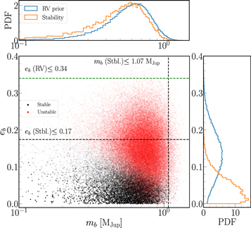
Figure 3 plots stability constraints on planet b, taking our 105 samples drawn from the mass and orbital eccentricity distributions reported by Suárez Mascareño et al. (2021). As with Figure 1, red points are configurations that went unstable in N-body integrations within 104 orbits, while the surviving black points have their opacity set according to their SPOCK probability of surviving for the next ≈20 Myr.
Figure 3. Stability constraints on planet b; masses and eccentricities were drawn from the Suárez Mascareño et al. (2021) RV posteriors (blue histograms), assuming the posteriors are Gaussian. Coloring and opacity scheme of the main panel follows the same as in Figure 1. Stability (orange histograms) strongly constrains the orbital eccentricity. The black dashed lines represent the 99.7th percentile upper limits from stability while the green dashed line depicts the RV Gaussian 3σ upper limit on the eccentricity (also shown in Table 2). The RV measured mass of 0.64 ± 0.19 is within a factor of 2 from the instability region even at zero eccentricity.
Download figure:
Standard image High-resolution image
We obtain a 99.7th percentile upper limit for mb of 1.07 MJup. Even though this upper limit is only ∼0.1 MJup lower than the Gaussian 3σ RV limit, we find that even if we extend our mass priors to higher values, masses above this limit are unstable at any eccentricity. Therefore, coincidentally, stability and RV observations yield very similar upper limits on planet b's mass. We also note that the median mass estimated through RV observations of 0.64 MJup (Suárez Mascareño et al. 2021) is within a factor of 2 from the stability limit even at zero eccentricity (Figure 3).
This implies strong stability constraints on planet b's orbital eccentricity, eb . We obtain a 99.7th percentile upper limit of 0.17 for the eb , which is half of the corresponding RV limit. Finally, we find that the constraints on planet b in Figure 3 do not depend strongly on the parameters for planets c and d (e.g., the bottom two rows of Table 2 comparing constraints for resonant and nonresonant configurations for c and d). This renders our approach of examining the configuration of planets c and d separately from those on planet b particularly valuable.
Table 2. 99.7th Percentile Upper Limits
| Parameter | Inside Resonance | Outside Resonance | RV (3σ) Reported |
|---|---|---|---|
| μ (MJup) | 0.94 | 0.35 | 0.55 |

| 0.17 | 0.06 | ⋯ |

| 0.02 | 0.02 | ⋯ |
| mb (MJup) | 1.07 | 1.07 | 1.21 |
| eb | 0.17 | 0.17 | 0.34 |
Note. 99.7th percentile upper limits. The second and third columns correspond to stability limits in the cases where planets c and d are inside and outside the 3:2 MMR, respectively (the left and right sides of Figure 1). The last column are the Gaussian 3σ RV limits reported by Suárez Mascareño et al. (2021). Bootstrap resampling of the stability posteriors gives errors on the order of ∼10−3 for each parameter.
Download table as: ASCIITypeset image
3.4. Is the System in an MMR Chain?
A challenge to establishing whether or not V1298 Tau is in an MMR chain is that the theory for MMR chains (e.g., Delisle 2017; Siegel & Fabrycky 2021) is less developed than for MMRs between a single pair of planets. We therefore take two approximate approaches.
First, we ask how many stable configurations place planets d and b (observed period ratio ≈1.946) inside the 2:1 MMR. In particular, when counting the fraction of configurations in the 2:1 MMR, we weight each one by its corresponding SPOCK probability of stability pi (Tamayo et al. 2021a):

This yields P(MMR chain) ≈ 1%. Even if future observations yield lower masses and eccentricities for planet b, the 2:1 MMR region lies at higher masses, making the system unstable. The fact that Pb /Pd ≈ 1.946, far from 2, is only in the 2:1 resonance region for the highest masses and eccentricities makes it even less likely that planets d and b are in the 2:1 resonance.
However, this analytical two-planet model ignores the gravitational effects of the third planet c, which can be important. We therefore instead check for libration of the three-body angle ϕchain = λc − 2λd + λb over timescales of 103 orbits of planet c, where the λ are the planets' mean longitudes. Using this libration condition to select configurations in the 2:1 MMR for the first sum of Equation (2), we obtain P(MMR chain) ≈0.02%. Both tests, therefore, rule out an MMR chain configuration for V1298 Tau at ≳99% confidence.
3.5. Ignoring Planet e
Similar to the stability step performed for planet b, we sampled the eccentricity and mass distributions of planet e from Suárez Mascareño et al. (2021) and the period distribution from Feinstein et al. (2021). We drew 105 samples from the stable configurations already with planet b, and we conducted uninformative and RV prior analysis similar to those we performed with planet b. In both cases, we found the inclusion of planet e does not affect the results of the inner planets, nor does stability constrain the period, mass, or eccentricity any better than what is already reported. The fact that plausible parameters for planet e do not affect our results justifies our choice to simplify the parameter space by excluding it.
4. Discussion and Conclusions
The theoretical work of Izidoro et al. (2017, 2021) posits that disk migration forms planetary systems in chains of MMRs, which subsequently destabilize as the protoplanetary disk disperses. Our finding that the currently youngest-known 3+ planet system V1298 Tau is not currently in an MMR chain configuration (≳99% confidence) suggests that either V1298 Tau did not follow this formation paradigm, or it constrains past dynamical instabilities to happening early—within the system's age of ≈20 Myr. Indeed, the first few Myr, during which disks disperse, present a natural time to drive instabilities as the stabilizing effects of the protoplanetary disk disappear (Izidoro et al. 2017, 2021).
One might ask whether an early instability is consistent with the present orbital architecture, in particular the near 3:2 period ratio of the inner two planets (c and d). We conducted limited N-body tests on a typical stable configuration by adding an additional body just outside planet b, and introducing enough eccentricity so that this new planet orbit crosses planet b. We found that the instability scenario typically ejected the additional planet from the system, and that it was consistent with the period ratios of the inner two planets if the hypothetical planet had a mass of less than ∼20 Earth masses. Indeed, a low mass would be required for the ejected planet in order to not leave the surviving planet b with too high an eccentricity (given our now more stringent constraints on its orbit).
Our conclusions are as follows:
- 1.Stability rules out an MMR chain at ≳99% confidence, assuming the RV mass and eccentricities from Suárez Mascareño et al. (2021). Lower values for these parameters further narrow the resonant region, diminishing the probability of planets d and b being in the 2:1 resonance. This implies that either the V1298 Tau planets did not form in an MMR chain, or if they did, they must have undergone a dynamical instability quickly following disk dispersal, within ≈20 Myr.
- 2.Figure 1 shows that the period ratio observations coupled with stability analysis can constrain the inner planet pair's combined mass. Additional sets of transits would help narrow down the resonant configuration and masses of the planets in the system.
- 3.If the inner two planets are in the 3:2 MMR, higher planetary masses require the planet pair to be closer to the resonance equilibrium (i.e., closer to the center of Figure 2).
- 4.The RV-measured mass for planet b is within a factor of 2 from the instability limit (see Figure 3). Stability places 99.7th percentile upper limits of 1.1 MJup and 0.17 for its mass and eccentricity, respectively.
Future observations of V1298 Tau will provide extremely valuable information on this landmark system, and we have provided a framework for incorporating complementary constraints from stability. While one cannot make general conclusions from a single system, this case study highlights the promise of ongoing searches for young planets in constraining our understanding of how planetary systems form and evolve over their Gyr lifetimes.
We thank Sam Hadden, Gumundur Stefánsson, and Adrian Price-Whelan for helpful discussions.
Software: celmech (Hadden 2019), corner (Foreman-Mackey 2016), Jupyter Notebooks (Kluyver et al. 2016), Matplotlib (Hunter 2007), NumPy (Van Der Walt et al. 2011; Harris et al. 2020), REBOUND (Rein & Liu 2012) SciPy (Virtanen et al. 2020), SPOCK (Tamayo et al. 2020).
Appendix: MMR Model
A.1. Reducing the Dimensionality
The dynamics near first-order MMRs depend on the orbital period ratio, masses mi , and eccentricity vectors e i (pointing in the direction toward the pericenter with a magnitude given by the eccentricity), where the subscript i indexes the planet. Two approximations simplify how the period ratio evolution depends on system parameters. First, Deck et al. (2013) show that the period ratio dynamics depend approximately only on the total mass of the planet pair divided by the stellar mass, μ = (m1 + m2)/m⋆ (and not the mass ratio m1/m2). For concreteness, we set planets c and d to have equal masses, but we have checked that varying the mass ratio does not significantly affect our results.
Second, the period ratio evolution depends primarily on a single linear combination of the eccentricity vectors e − (Sessin 1983; Henrard 1984; Hadden 2019),

where f and g are Fourier coefficients in the disturbing function expansion of the interplanetary potential (e.g., Hadden 2019). The approximation that e − is nearly the vector difference e 2 − e 1 is excellent for all first-order MMRs except the 2:1 (in which the relationship between f and g is altered by additional indirect terms that need to be considered), and can thus be thought of as a relative or antialigned eccentricity. This transformation additionally defines a combined pericenter ϖ−, which approximately specifies the longitude at which the two orbits come closest to one another.
The remaining linear combination of eccentricities, which can be expressed as an approximately conserved center-of-mass eccentricity (e.g., Hadden 2019), to excellent approximation does not affect the period ratio evolution for a single pair of planets on short timescales. However, larger values of this center-of-mass eccentricity do affect stability in multiplanet configurations, by leading to larger secular oscillations in e− on longer timescales (Tamayo et al. 2021b). In order to limit the parameter space, we set the center-of-mass eccentricity to zero as a best-case scenario for stability. Our derived upper limits on masses and orbital parameters in this best case are thus conservative and reliable.
A.2. Physically Meaningful Parameters
For a period ratio near an MMR commensurability, different masses, eccentricities, and pericenter orientations will lead to oscillations in the period. However, there always exists a resonant equilibrium corresponding to a particular combination of the above parameters, where the period ratio remains constant.
To a good approximation, for a given j: j − 1 MMR, the equilibrium, or forced, eccentricity eforced is only a function of the equilibrium period ratio and μ (e.g., Hadden 2019). In addition the equilibrium resonant angle ϕ = j λ2 − (j −1)λ1 − ϖ−, which approximately measures the location at which conjunctions occur, is always at ϕ = π. This corresponds to conjunctions occurring at the location where the two orbits are farthest from one another.
Initial conditions near, but not at, the resonant equilibrium will oscillate around it. The antialigned eccentricity e− can thus be profitably decomposed into free and forced components (e.g., Murray & Dermott 1999),

In this picture, eforced is the equilibrium value at which the antialigned eccentricity and period ratio would remain constant (if ϕ = π), and the free eccentricity efree is how far away the eccentricity is from the fixed point. Additionally, the forced eccentricity is a conserved quantity involving both e− and the period ratio's deviation from the resonant value (in this case Pd /Pc = 3/2), which lets one switch back and forth between the two variables.
Because various configurations with different resonance strengths can have very different values of eforced, but the equilibrium period ratio is always approximately 3/2, we choose in Figure 2 to plot the period ratio deviation δ P. The center at (ϕ, δ P) ≈ (π, 0) is the equilibrium, corresponding to different nonzero values of eforced for each configuration (point). Points near the equilibrium approximately execute circles around the fixed point, allowing for a simple scalar distance from the fixed point to parameterize the oscillation amplitude. At larger distances from the resonant fixed point, the trajectories become more deformed, and can even oscillate around a different fixed point. Since the distance from the equilibrium therefore varies for general, noncircular trajectories, we define efree to be the value for the trajectory (through Equation (A2)) when the resonant angle ϕ crosses through π, and we convert it to a period deviation with celmech to make Figure 2.
In order to account for the phase of oscillations to match the observed period ratios (the bottom panels of Figure 1), we initialize the system with total mass ratio μ, and eforced and efree at ϕ = π (i.e., along a vertical line in Figure 2). We then integrate the orbits using the REBOUND N-body integrator (Rein & Liu 2012) for a uniformly drawn time ΔT, which we marginalize over when presenting the posterior distributions in Figure 1.
A.3. Resonant versus Nonresonant Configurations
While libration of the resonant angle ϕ is often used as a test of whether a pair of planets is in resonance, this distinction is not physically meaningful when the MMR is weak (i.e., in these cases there is no dynamically meaningful difference in behavior between a configuration where ϕ circulates, and one where it librates with a large amplitude). A more meaningful distinction is to separate this question into two parts.
First, there is a threshold strength for first-order MMRs (parameterized by μ and eforced), beyond which a separatrix appears (e.g., Henrard 1984; Deck et al. 2013). This separatrix trajectory is (in the analytic approximation of the MMR model) an infinite-period trajectory (black "cat's-eye" curve in Figure 2). Configurations inside the separatrix (small efree) are resonant, and cleanly separated from nonresonant trajectories (large efree) on the outside. This is a physically important boundary because trajectories near the separatrix are most susceptible to chaos under perturbation (e.g., Lichtenberg & Lieberman 1992; Rath et al. 2021). When the MMR is weak, i.e., below the threshold MMR strength, there is no separatrix, and there is no dynamically meaningful boundary between resonant and nonresonant configurations.
We therefore use the celmech package to calculate whether a separatrix exists or not for each of the orbital configurations in Figure 1. If it does, we use the fact that the numerical value of the (conserved) Hamiltonian for a resonant trajectory (inside the separatrix) is always smaller than the value on the separatrix. On the left side of Figure 1, we then plot all the configurations where (a) a separatrix exists and (b) the value of the Hamiltonian places it inside the resonant region. All remaining configurations are then plotted on the right side of Figure 1, i.e., (1) cases where the MMR is so weak there is no separatrix and (2) cases where a separatrix does exist, but the system is outside the resonant region.
Footnotes
- 1
Jupyter notebooks and scripts used in our analysis can be found in https://github.com/Rob685/V1298Tau_stability.
- 2
Dropping a scaling offset term that does not affect the rejection sampling.
- 3
Detailed API: https://github.com/shadden/celmech.