Uncertainty definitions
1,761 views
Skip to first unread message

Stefan Gächter
Jan 23, 2021, 4:32:00 AM1/23/21
to gtsam users
I am digging into some details of GTSAM to get a better understanding, in particular, on the details of the BetweenFactor.
The first conceptual difference I noted is that residuals are defined for the BetweenFactor as prediction minus measurement - estimate minus observation - whereas in photogrammetry or classical Kalman filter it is the opposite, that is observation minus estimate. In photogrammetry, observation plus estimate would be a correction.
To my understanding, the residuals as prediction minus measurement stems from the conventions in group theory, where left hand operators are preferred, and GTSAM is beautifully built up on this.
Having a Kalman filter background, I got first confused about the uncertainty definition of the measurement of the BetweenFactor. I found the frame conventions document in the repository - though, it was not an easy read for me - helped me to clarify my confusion.
A short example:
Given two poses i and j in world frame: wXi and wXj
Then then the between pose is iXj = wXi^-1*wXj, it is the delta pose in frame i
The measurement of this delta pose is iZj
So, the between factor would look like BetweenFactor(i, j, iZj, sigma)
The residuals of the between factors are then jRj = iZj^-1*iXj
As one can see here, the residuals are in frame j. Therefore, uncertainty has to be in frame j as well. - For a classical Kalman filter, it would be frame i.
The above mentioned document states "implies that the measurement is in frame x, i.e. it measures y in x, and that the uncertainty is in the frame of the measurement, or equivalently, in frame y" What I do not understand here is "uncertainty is in the frame of the measurement" Isn't the frame of measurement frame i, because it is iZj? But then it is not equivalent to frame j of wXj, no?
What I could not find - or I did not dig enough - was how the noise has to be specified for Pose2 and Pose3.
My understanding is for Pose2: Diagonal.Sigmas([x, y, theta]), so, first position, then rotation,
and for Pose3: Diagonal.Sigmas([alpha, beta, gamma, x, y, z]), so, first rotation, then position.
Is my understanding correct? Please let me know, if this is outlined somewhere.
Thanks again for all the effort you put into this library.
Thanks again for all the effort you put into this library.
Kind regards
Stefan

Matías Mattamala
Jan 23, 2021, 8:49:39 AM1/23/21
to gtsam users
Hi Stefan,
I've had this confusion as well. I'll try to answer your questions below.
1. Regarding the conventions
As you said, GTSAM is built upon Lie group theory. That requires to assume one convention to apply some operations - left or right handed.
GTSAM uses right-hand notation: corrections are applied on the right hand, as well as right jacobians are chosen in general. Probability distributions of elements of the group are also defined with "right notation".
With a concrete example, let's say you have a Pose3 (i.e, a rigid-body matrix, an object from SE(3)) that represents the pose of the body in time 1 in the world frame: w_T_w_b1
Additionally, you have another estimate at time 2: w_T_w_b2
You additionally have a measurement of the relative pose between 1 and 2 (like, an odometry measurement). Let's be ambiguous for now and call it dT
With the previous information, the following expression holds.
w_T_w_b2 = w_T_w_b1 * dT
If we make an analogy with a common Kalman filter scheme, it's like a process model:
x(t+1) = x(t) + u(t)
However, the previous equations are deterministic - we're not considering noise nor any distribution. We want things to be Gaussian, so in the Kalman filter case we say that the control u(t) has some white noise n (i.e, zero mean Gaussian noise, with covariance sigma):
x(t+1) = x(t) + u(t) + n
So if you take the previous equation, an leave the noise alone, you can say that the difference distributes as a zero mean Gaussian with covariance sigma:
x(t+1) - x(t) + u(t) = n
So what you end up having on the left hand side, is basically a vector version of the between factor. You can directly use it in GTSAM using the covariance sigma as the factor covariance.
Now the thing is to make the same when you have poses. We have this equation:
w_T_w_b2 = w_T_w_b1 * dT
We say that the only source of noise is the measurement dT. So we "add" a zero mean Gaussian noise:
w_T_w_b2 = w_T_w_b1 * dT * Exp(N)
The new term, Exp(N) is the exponential map of a variable N that distributes as a zero mean Gaussian, but on the tangent space of the group. It means that it has 6 degrees of freedom (3 position + 3 orientation), and has a covariance matrix Sigma6 (6x6).
Now this new term is the only source of uncertainty. Let's isolate as before to obtain our between factor and analyze what happens:
(dT)^-1 * (w_T_w_b1)^-1 * w_T_w_b2 = Exp(N)
The inversion (w_T_w_b1)^-1 results in b1_T_b1_w (we flip the frames)
=> (dT)^-1 * b1_T_b1_w * w_T_w_b2 = Exp(N)
The blue term basically defines the difference between frames 1 and 2, defined in frame 1
To make this consistent, (dT)^-1 should match the frames, so it should be
dT^-1 = b2_dT_b2_b1
Hence, dT must be dT = b1_dT_b1_b2
dT describes a transformation defined in b1 that "takes you" to b2 - what an odometry measurement is supposed to do.
The whole error (between factor) is finally:
(b1_dT_b1_b2)^-1 * b1_T_b1_w * w_T_w_b2 = Exp(N)
Which is defined "in b2 to b2". So it must be Exp(N) the error on the right hand side, hence its covariance Sigma. That's why we said the error is defined on the measurement frame, i.e, b2 in this example.
It is quite critical to keep track of the frames of the transformations and measurements involved when the objects are rigid-body transformations, rotation matrices or quaternions. However, this doesn't happen only in factor graphs, but Kalman filters too, because it depends how you apply the corrections and the noise.
The previous example implicitly adopted a right hand notation when defining:
w_T_w_b2 = w_T_w_b1 * dT * Exp(N)
We could have also expressed:
w_T_w_b2 = w_T_w_b1 * Exp(N) * dT
But that would have implied "noise defined in frame b1" which could make things more involved. GTSAM always assumes that noises are applied from the right hand side.
As a last remark on this side, the expression dT * Exp(N) is also interpreted as a Gaussian with mean dT and covariance Sigma. This is also a right hand notation to express distributions on SE(3).
2. Regarding how the noise must be defined for each factor, when I'm confused I always check the Logarithm map implementation of each object.
Most of the factors that require working with Lie Groups usually have a Logarithm map that converts the matrix difference into a vector difference by mapping the difference to the tangent space.
As we said before, since the tangent space is has the same dimension of the minimum representation of the object (rotations 3, poses 6, etc), the covariance should match their dimension, and the Logarithm map resulting vector should follow the order in which the covariance matrix must be defined.
In particular, what you said is right
- Pose2 is (x, x, theta)
- Pose 3 is (alpha, beta, gamma, x, y, z)
3. Lastly, I think that handling the covariances is always tricky because we need to be careful with the conventions.
While GTSAM uses right hand, others use left hand. For instance, this pretty nice paper shows you how to compute the covariance of a difference of distributions, composition, inverses and so on, but it uses a left hand notation. So you must adapt the equations to be consistent with GTSAM for example.
I hope it helps!
Matias
I hope it helps!
Matias

Dellaert, Frank
Jan 23, 2021, 10:38:28 AM1/23/21
to Matías Mattamala, gtsam users
Hi both
This is awesome, and I acknowledge this is probably not explained well in the docs. If you both are interested in writing this up in markdown, we can both add it to the docs and feature it as a blog post on gtsam.org?
BTW, GTSAM used to be based on Lie groups. After reading Absil et al, it is now really based on manifolds and retractions. For Lie groups, the default retraction is indeed the right-side multiplication with exp(xi), with xi in tangent space.
Frank
From: gtsam...@googlegroups.com <gtsam...@googlegroups.com> on behalf of Matías Mattamala <matt...@gmail.com>
Sent: Saturday, January 23, 2021 08:49
To: gtsam users <gtsam...@googlegroups.com>
Subject: [GTSAM] Re: Uncertainty definitions
Sent: Saturday, January 23, 2021 08:49
To: gtsam users <gtsam...@googlegroups.com>
Subject: [GTSAM] Re: Uncertainty definitions
--
You received this message because you are subscribed to the Google Groups "gtsam users" group.
To unsubscribe from this group and stop receiving emails from it, send an email to gtsam-users...@googlegroups.com.
To view this discussion on the web visit https://groups.google.com/d/msgid/gtsam-users/d35b8785-4f8c-4ddf-b2b4-f9feb9efb3ffn%40googlegroups.com.
Matías Mattamala
Jan 23, 2021, 10:47:22 AM1/23/21
to gtsam users
Hi Frank,
I'd be happy to work on that. I can start writing up a draft if we are ok with it.
And thanks for the clarification on GTSAM, I'll take a look at the book.
Matias
I'd be happy to work on that. I can start writing up a draft if we are ok with it.
And thanks for the clarification on GTSAM, I'll take a look at the book.
Matias
Stefan Gächter
Jan 25, 2021, 5:53:24 AM1/25/21
to gtsam users
Dear Matias,
Thanks a lot for your detailed explanation. I went through it and, I think, we have a common understanding.
I have some follow-up questions, though.
I have some follow-up questions, though.
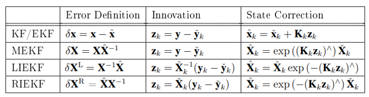
About the notion of left and right, the following table is from Thesis | Practical considerations and extensions of the invariant extended Kalman filtering framework | ID: 6h440z107 | eScholarship@McGill
Table 3.1, page 37.
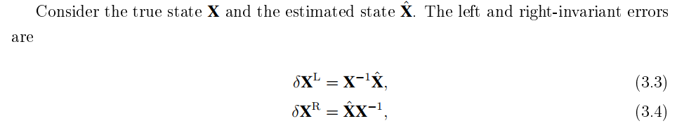
where the definitions of left and right errors are, page 19,
To my understanding, GTSAM uses the left-invariant error (3.3), no?
The left-invariant error would correspond to (b1_dT_b1_b2)^-1 * b1_T_b1_w * w_T_w_b2 = Exp(N), no?
If yes, then it would be left-invariant error, but right-hand notation?
About the measurement for the between factor, using your notation, it would be implemented as
b1_T_b1_b2 = (w_T_w_b1)^-1 * w_T_w_b2
BetweenFactor(1, 2,
b1_T_b1_b2 , sigma)
To my understanding, b1_T_b1_b2 is the measurement. The measurement b1_T_b1_b2 is in the body-frame b1, no?
I agree that uncertainty (b1_dT_b1_b2)^-1 * b1_T_b1_w * w_T_w_b2 = Exp(N) is in the body-frame b2. But, for me, this is not the same as the measurement.
Thanks for the clarification. For Pose3, it is rotation, then position.
What I do not yet know is, what minimal representation is used for the rotation? Or asked differently, what are the components (alpha, beta, gamma)? Are this the components of axis-angle/Rodrigues-vector representation?
I tried to figure that out from the source code, but have failed so far.
I am wondering how much people consider these details. It was a big learning for me. And from my experience with some experiments, it does not matter much, if noise is assumed isotropic, but as soon as the noise is non-isotropic, the problems start to pop-up.
Thanks again for your time and effort. I would be happy, if I can contribute something.

José Luis Blanco-Claraco
Jan 25, 2021, 6:16:00 AM1/25/21
to Stefan Gächter, gtsam users
Dear Stefan, Matías:
I think this thread is also relevant to this interesting discussion
(and in particular, to your last question on what are the components
alpha, beta, gamma):
https://github.com/borglab/gtsam/issues/504
JL
I think this thread is also relevant to this interesting discussion
(and in particular, to your last question on what are the components
alpha, beta, gamma):
https://github.com/borglab/gtsam/issues/504
JL
Matías Mattamala
Jan 25, 2021, 6:42:37 AM1/25/21
to gtsam users
Hi Stefan, José Luis,
I'm happy to know it helped. Thanks for sharing the issue as well, I'll definitely take a look, perhaps there is something I'm missing.
Regarding Stefan's follow-up questions:
1. Yeah, I think I agree with you that according to the definitions, it would be left-invariant error, but "right convention"
if you define the state X as w_X_wb, and w_X'_wb to represent the estimated state, then the "left invariant error" is error defined in the base frame: w_X_wb^-1 * w_X'_wb
So it makes sense to apply the correction to the estimate on the right using the Exponential map
2. Regarding the implementation
- Yes, BetweenFactor(1, 2, b1_T_b1_b2 , sigma) should work
- While measurement b1_T_b1_b2 is gonna be expressed in frame b1, it represents a transformation "that transforms elements expressed in frame b2 to frame b1". The tricky part here is that while the measurement itself is expressed in a frame (base 1), its covariance is expressed in a different one (base 2), because the measurement itself is changing the frames. This doesn't happen when you have vectors, because you can add vectors (noise in this case) either from the left or the right and it works. Perhaps that's the source of the confusion.
3. Minimal representation
I tend to think that the minimal representation of orientation (tangent space) is Axis-Angle, since the exponential map is usually defined as the Rodrigues rotation formula. And I try to avoid thinking in Euler angles because all their conventions confuse me :(
Best,
Matias
Stefan Gächter
Jan 25, 2021, 7:42:40 AM1/25/21
to gtsam users
Thanks, Jose Luis, for pointing to the discussion. I have yet to study your example.
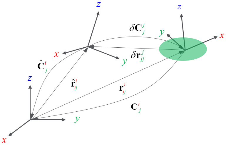
I made a drawing to understand better the frames. Sorry, yet another notation. The bewteen factor residuals are j_r_jj and j_C_j for position and rotation, respectively. The green ellipse should indicated the uncertainty. As one can see, the uncertainty is defined in j-frame to include the residual.
Thanks, Matias, indeed, 2) is an important point. About 3), so, my understanding is correct that the covariance - sigmas provided to BetweenFactor - is the covariance of the axis-angle representation and not of Euler angles, right?
Matías Mattamala
Jan 25, 2021, 7:56:01 AM1/25/21
to gtsam users
Hi again,
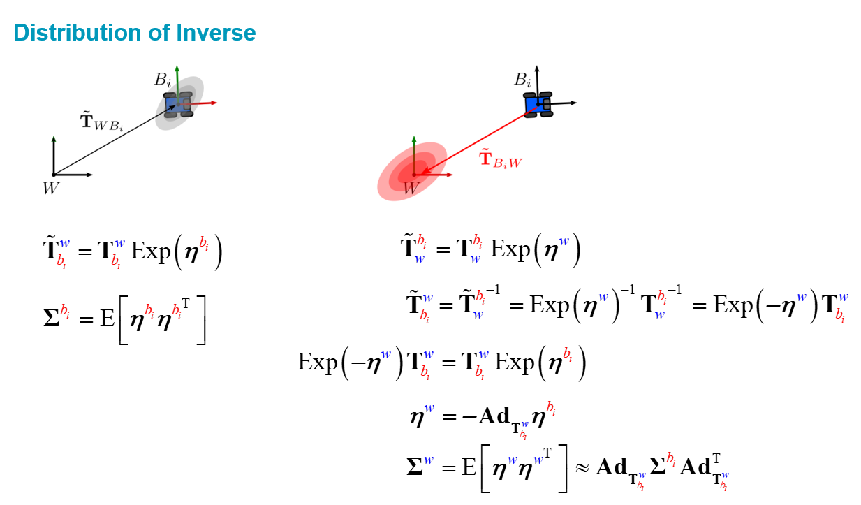
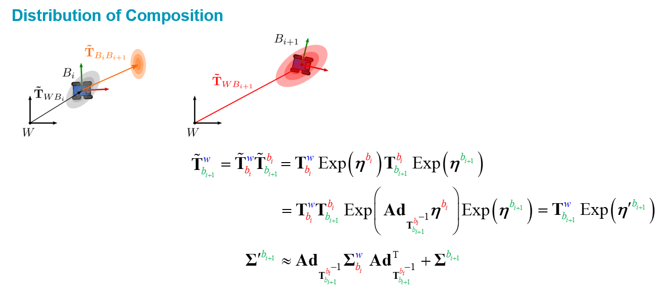
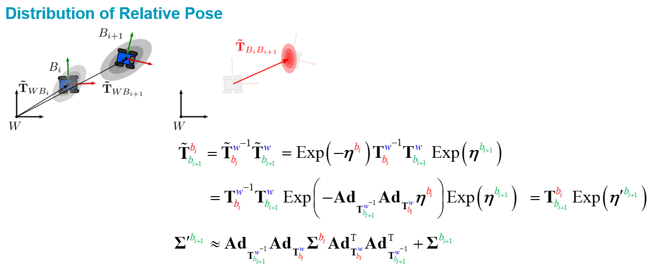
I was about to share some slides with figures, since we were having the same discussion with my group about uncertainties this morning (such a coincidence).
From your figure, I understand (let me know if I'm right):
- i is the frame at the left
- j is the frame at the center
- the frame at the right is the pose of the robot/vehicle
- j_r_jj and j_C_j are the odometry measurements that move the robot away from frame j, relative to the same frame.
If I got all of that ok, yes, the covariance/uncertainty will be defined as you did. This is locally valid in j, if you want to express it in i you need to transform it with the Adjoint (the slides above suggest some procedures)
Regarding the last question, yes, the covariance should be axis-angle. We're not using Euler angles at all in the tangent spaces (but probably there are some conditions/conventions under which they are the same as Euler angles)
Best,
Matias
Dellaert, Frank
Jan 25, 2021, 8:53:46 AM1/25/21
to Matías Mattamala, gtsam users
Matias
great slides!
Frank
From: gtsam...@googlegroups.com <gtsam...@googlegroups.com> on behalf of Matías Mattamala <matt...@gmail.com>
Sent: Monday, January 25, 2021 07:56
To: gtsam users <gtsam...@googlegroups.com>
Subject: Re: [GTSAM] Re: Uncertainty definitions
To: gtsam users <gtsam...@googlegroups.com>
Subject: Re: [GTSAM] Re: Uncertainty definitions
To view this discussion on the web visit
https://groups.google.com/d/msgid/gtsam-users/19892ef4-f8fd-4487-a28a-1fb8d3e10fc9n%40googlegroups.com.
Stefan Gächter
Jan 25, 2021, 9:34:59 AM1/25/21
to gtsam users
Yes, thanks for the slides. It helped me to solidify my understanding.
Ok, understood that with the tangent space now.
Ok, understood that with the tangent space now.
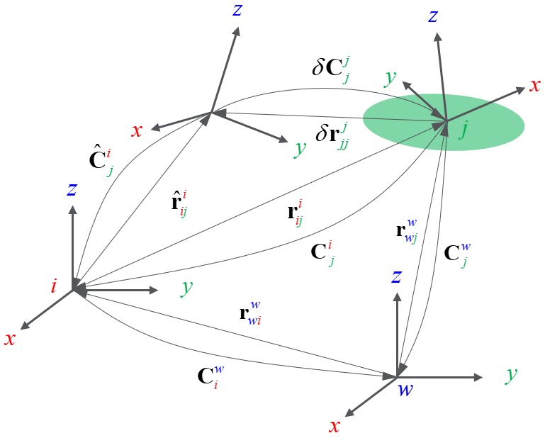
Sorry, my figure was not clear. It showed the delta pose measurement. The complete figure should be:
Matías Mattamala
Jan 25, 2021, 10:15:37 AM1/25/21
to gtsam users
Thank you Frank and Stefan, I'm glad it helped.
Yeah, taking a deeper look at the figure, it would be correct. Ideally dC_jj and dr_jj should be zero (residual zero) and exactly match the pose of frame j. But in reality there could still exist a difference -that is explicit in your diagram-, which is handled by assuming that the measurement follows some distribution (with the green covariance).
Yeah, taking a deeper look at the figure, it would be correct. Ideally dC_jj and dr_jj should be zero (residual zero) and exactly match the pose of frame j. But in reality there could still exist a difference -that is explicit in your diagram-, which is handled by assuming that the measurement follows some distribution (with the green covariance).

KUNTAL GHOSH
Jan 28, 2021, 9:24:40 PM1/28/21
to gtsam users
Hello Frank,
Can you share your paper titled "Factor Graphs: Exploiting Structure in Robotics"? It will be real help for me.
Thanks

Mike Bosse
Feb 8, 2021, 11:07:17 PM2/8/21
to Matías Mattamala, gtsam users
Hi All,
I'm getting the sense that this discussion is making things more complicated than necessary. The figure with two arrows for the transformation between frames really clutters things, and it is a lot cleaner to just look at a single object to represent the transformation between two frames. (ie i_T_j)
For the uncertainty representation, all one needs to look at is the definitions of the `local` and `retract` functions which together define the tangent space for the group:
v = local(A,B)
B = retract(A,v)
where A and B are two group objects, and v is a vector in the tangent space at A.
For three dimensional transformations there are several possible conventions, and gtsam uses the right tangent space convention (see Pose3.cpp):
local(w_T_a, w_T_b) = logmap(w_T_a^-1 * w_T_b)
retract(w_T_a, v) = w_T_a * expmap(v)
where (depending on the preprocessor defines) logmap and expmap are the SE(3) log and exp operators.
These functions are also where the order of the dimensions in the tangent space can be figured out. (which is rotations first for Pose3, but last for Pose2)
The key to understand the uncertainty for any factor is to look at the tangent space of the measurement's group.
So for a BetweenFactor(w_T_i, w_T_j) the measurement is modeled as i_T_j = w_T_i^-1 * w_T_j. And since the tangent space (for gtsam::Pose3) is on the right, one can think of the uncertainty as being in j's coordinate frame.
It is only a coincidence that both the between factor and the Pose3 tangent spaces are defined on the left. It would not difficult to define one's own version of the Pose3 class that uses a different tangent space definition; for example if it the retract were defined as a correction on the right: w_T_b = expmap(v) * w_T_a, then the BetweenFactor's uncertainty would be in i's coordinate frame.
I hope that helps a little...
Mike Bosse / Senior Manager, CLAMS Algorithms / Zoox / +1 408 718 7200
To view this discussion on the web visit https://groups.google.com/d/msgid/gtsam-users/45c26321-0218-4432-b897-d5edf10ac1een%40googlegroups.com.
Mike Bosse
Feb 8, 2021, 11:58:15 PM2/8/21
to Matías Mattamala, gtsam users
Oops, in my last paragraph, I accidentally swapped 'left' and 'right'; It should read:
"It is only a coincidence that both the between factor and the Pose3 tangent spaces are defined on the right. It would not difficult to define one's own version of the Pose3 class that uses a different tangent space definition; for example if it the retract were defined as a correction on the left: w_T_b = expmap(v) * w_T_a, then the BetweenFactor's uncertainty would be in i's coordinate frame."
Sorry for the dyslexia
Stefan Gächter
Mar 25, 2021, 12:13:18 PM3/25/21
to gtsam users
Thanks, Mike, for your comment. Meanwhile familiar with manifolds and groups, I agree that it is wise to look at the tangent space first.
Stefan Gächter
Mar 25, 2021, 12:26:31 PM3/25/21
to gtsam users
Thanks
a lot , Matias, and all who have contributed, for the three part tutorial. You put everything nicely together and it consolidated my understanding. It was a treat to read it.
One thing, which I do not yet fully understand, though, is, how the distribution looks like. Equation (32) states the following
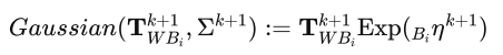
One thing, which I do not yet fully understand, though, is, how the distribution looks like. Equation (32) states the following
where
If I understand it correctly, then the distribution in the tangent space is Gaussian. But also on the manifold.
Is there a simple proof? Sorry, maybe this a trivial question.
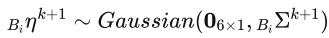
My confusion comes from the "banana distribution" I have endorsed (from Long's RSS'08 paper):
Is there a simple proof? Sorry, maybe this a trivial question.
My confusion comes from the "banana distribution" I have endorsed (from Long's RSS'08 paper):
But maybe I mixing things up.
Matías Mattamala
Mar 25, 2021, 1:04:28 PM3/25/21
to gtsam users
Hi Stefan,
I'm glad to know the posts were helpful :)
Yes, I understand the question. The distribution on the tangent space is indeed Gaussian in the "normal sense", like an ellipse, or ellipsoid when you have higher dimensions, because the tangent space is Euclidean.
However, when you apply the exponential map, we still say it's a "Gaussian on the manifold" but if you actually try to plot it in an Euclidean space (as in the RSS paper, using sampling for instance), you will see that the shape is not an ellipsoid but a "banana distribution" as you pointed out. This fact -plotting a manifold, with specific constraints, into Euclidean axes- is what causes this mismatch with the intuition.
I hope this helps to solve the question.
Best,
Matias
Stefan Gächter
Apr 20, 2021, 5:02:11 AM4/20/21
to gtsam users
Thanks, Matias, I finally got it.
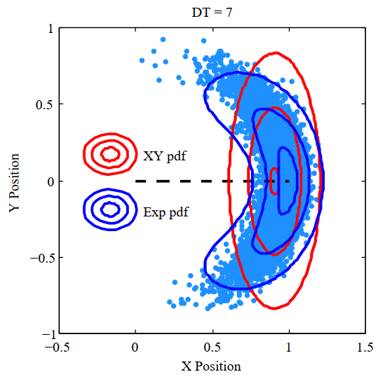
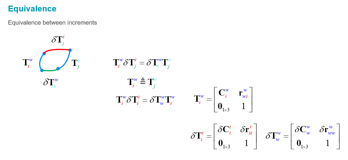
I am taking a closer look at adjoints and I got stuck with the notation. May I ask for some clarification in part 3?
Isn't the combination of equation (1) and (2) resulting equivalence in the following way?.gif?part=0.2&view=1)
.gif?part=0.3&view=1)
.gif?part=0.1&view=1)
I am taking a closer look at adjoints and I got stuck with the notation. May I ask for some clarification in part 3?
Isn't the combination of equation (1) and (2) resulting equivalence in the following way?
where V is Wi and C is Bi. Exp() is a transformation. Therefore, I added the subscript WV and CB to the increment.
Then, the assumption is
Thus
where C is B, which corresponds to equation (3).
Left and right increment are becoming transformation on itself.
Left and right increment are becoming transformation on itself.
How to say, if sticking the the notation of as outlined in part 2, then it is not obvious for me to get equation (3). The transformation is becoming somehow a pure rotation. Not sure, if I expressed myself clearly.
Stefan
Stefan Gächter
Apr 23, 2021, 8:43:59 AM4/23/21
to gtsam users
Hm, maybe my previous question does not make much sense. The normal distribution is not a transformation and, thus, my notation does make much sense.
I think there is a type in Part 3, equation (15) and (17). To my understanding, it should be Sigma_{B_i} on the right hand side, not Sigma_{B_{i+1}}
Still, another question, in equation (5), why is it the adjoint of the inverse T^{-1}? I studied the paper of Sola and where, to my understanding, it is the adjoint of T. At least, from a notation point of view.
Matías Mattamala
Apr 24, 2021, 9:01:01 AM4/24/21
to gtsam users
Hi Stefan,
I'm not sure I got the previous question fully (the one where you shared the equations) but let me know if you want to discuss it further. I think that's one of the weakest parts of the posts, so I'm happy to discuss it further to make it clearer.
Regarding Equation (15) and (17) you're absolutely right, there is a notation problem that makes things confusing. Thanks for pointing this out. Someone else also made me notice and I'll fix it.
The last question about Sola, if you meant equation (32) in the paper I think that both are right. I'll use the same notation as the blog post to show it:
Sola uses X⊕t = (Ad_X * t) ⊕ X. Using the notation of the posts, this is equivalent to:
T_w_b * Exp(b_xi) = Exp(Ad_T_w_b * b_xi) T_w_b
So he wants to move an increment defined on the right, to the left hand side. In this case, we use the adjoint of T_w_b (no inversion), because that transforms b_xi into Ad_T_w_b * b_xi (in world frame), which matches the frame on the left of T_w_b. We can use the same subindex cancelation trick to confirm the frames are consistent (the only frame that remains is w on the left)
On the other hand, I used the opposite. I wanted to move an increment defined on the left w_xi, to the right hand side:
-> Exp(w_xi) * T_w_b = T_w_b * Exp(Ad_(T_w_b)^{-1} * w_xi)
-> Exp(w_xi) * T_w_b = T_w_b * Exp(Ad_T_b_w * w_xi)
The inversion swaps the indices and then Ad_T_b_w * w_xi represents an increment defined in the base, which matches the frame on the right of T_w_b
You can also confirm it if you concatenate both operations starting from Sola's, moving the increment to the left, and then back to the right using the one in the post:
T_w_b * Exp(b_xi) = Exp(Ad_T_w_b * b_xi) T_w_b // Sola
= Exp(Ad_T_w_b * b_xi) T_w_b // Increment now in world frame
= T_w_b * Exp(Ad_T_w_b^{-1} * Ad_T_w_b * b_xi) // Blog post's to move the increment to the right
= T_w_b * Exp(Ad_T_b_w * Ad_T_w_b * b_xi) // Inverting and swapping indices
= T_w_b * Exp(Ad_T_b_w * Ad_T_w_b * b_xi) // Now everything is in base frame and the adjoints cancel each other
= T_w_b * Exp(b_xi)
I hope it helps, and thanks again for noticing the typos :)
Stefan Gächter
Apr 27, 2021, 4:03:23 AM4/27/21
to gtsam users
Thanks, Matias, for your derivations.
I had a look again at my derivations and, I beg your pardon, I made a mistake. Firstly, your derivations correspond perfectly with Sola's one, as you showed.
Secondly, equation (15) and (17) are correct, but could be improved for readability by adding an apostrophe.
Here, my derivations, which should match yours, maybe helpful for others:
Sorry for the inconvenience. I should have checked more carefully my eqations.
Actually, the PhD thesis of Rodriguez Arevalo, On
the Uncertainty in Active SLAM: Representation, Propagation and Monotonicity, https://dialnet.unirioja.es/servlet/tesis?codigo=257909, helped me a lot to cross-check the derivations.
My confusion was caused by the notation of noise terms. Maybe following slide explains my first question:
The increments dT do not transform from one to another coordinate frame, but end up in the same coordinate frame. I haven't found a good way to explain, but using the transformation notation to describe the small increments or the distribution confuses me, because it is not meant as a from-to-transformation.
Matías Mattamala
May 11, 2021, 9:48:25 AM5/11/21
to gtsam users
Hi Stefan,
No worries at all, I'm happy to know we conclude the same. Thanks again for the feedback in those equations, it's confusing indeed.
I also agree that the increments/corrections are not that straightforward to interpret. While it's tempting to define them as a from-to-transformation, it doesn't make sense in the end as you mentioned and I haven't figure out a better way to explain it either. In the blog post I decided to use only the frame in which the increment is defined, but the interpretation is up to the reader.
Reply all
Reply to author
Forward
0 new messages